
Ansari Bradley Test: 7 Essential Steps, Formula and Worked Example
The Ansari Bradley test is a nonparametric two-sample dispersion test for deciding whether two independent populations have the same scale. This complete guide covers the Ansari Bradley test assumptions, the symmetric-score statistic, the large-sample and permutation calculations, an applied final-grade example, interpretation, and reproducible workflows in Python, R, SPSS and Excel.
Scale / dispersion
Rank-based
Ties handled
Python + R + SPSS + Excel
No statistically significant difference in dispersion was detected.
In this worked Ansari Bradley test example, final grade (G3) was compared between students without family educational support (n = 251) and students with support (n = 398). Both groups had a median of 12, satisfying the most important observed location check. The Ansari Bradley test statistic was A = 40,094.50; the tie-adjusted large-sample calculation gave |z| = 0.646 and p = 0.518, while the permutation result was p = 0.511. At α = .05, equal scale was not rejected.
What does the Ansari Bradley test measure?
A rank-based answer to a scale question, not a general test of any distributional difference.
The Ansari Bradley test answers a narrow but important question: after assuming a common population location and comparable standardized shape, is one independent population more dispersed than the other? It is a two-sample scale test, not a general replacement for a t test, Mann–Whitney test or equality-of-distributions test.
The research question
The Ansari-Bradley two-sample test evaluates whether two independent populations have the same scale parameter. In practical work, scale is usually discussed as spread, variability or dispersion. A wider population distribution has a larger scale; a tighter distribution has a smaller scale.
The test is especially useful when the outcome is non-normal, heavy-tailed, ordinal with many distinct values, or otherwise unsuitable for an F test. It uses the order of the pooled observations rather than squared deviations from a mean.
What it does not test
It is not a test of mean differences, median differences, stochastic dominance or overall equality of distributions. Those are different questions. The test’s clean scale interpretation requires the groups to have a common location and comparable distributional shape apart from scale.
When the medians differ, a significant Ansari-Bradley result can reflect location contamination rather than a pure dispersion difference. That limitation is central, not optional.
When should you use the Ansari Bradley test?
Use the decision logic below before opening software.
Use the Ansari Bradley test only when the research target is dispersion for exactly two independent samples. The choice should come from the estimand and design—not simply from a failed normality test or from a desire to avoid reporting unequal variances.
Two groups?
The method is designed for exactly two independent samples.
Numeric or ordinal?
The outcome must be orderable and should contain enough distinct values to support ranking.
Independent units?
No participant, school, device or experimental unit should contribute to both groups.
Common location?
The population medians should be equal or a defensible location difference should already be known.
Scale question?
Your hypothesis must concern dispersion, not a difference in central tendency.
Good uses
Do not use it automatically
Ansari Bradley test assumptions: six conditions to check
The method is nonparametric, but it is not assumption-free.
The Ansari Bradley test assumptions determine whether the rank statistic can be interpreted as evidence about scale. Independence, an orderable outcome, a common location, comparable shape and transparent tie handling are substantive requirements rather than a checklist added after the p-value is known.
Independent samples
Observations must be independent within and between groups. Clustered, matched or repeated observations require a different design-aware method.
Ordered outcome
The variable must be at least ordinal. Continuous measurements are ideal; many ties reduce information and affect exact inference.
Equal location
The groups should have the same population median, or their known location difference should be removed before the test.
Comparable shape
For a pure scale interpretation, the distributions should have the same basic form after accounting for location and scale.
Random sampling
The observations should arise from a design that supports population inference, such as random sampling or random assignment.
Ties handled explicitly
Tied values require averaged symmetric scores and an adjusted variance or a permutation approach designed for ties.
Nonparametric does not mean “works for any data.” See parametric vs nonparametric tests for a broader explanation of what distribution-free procedures do and do not guarantee.
Ansari Bradley test hypotheses: population scale, not sample SD
State the null in the common-location scale model and then translate it into the variables being analyzed.
The Ansari Bradley test does not literally test whether the two observed standard deviations are numerically equal. It tests whether two independent population distributions have the same scale parameter under a model in which they share a common location and standardized shape.
Formal location–scale model
Let the first population represent G3 for famsup = no and the second represent G3 for famsup = yes. A clean scale interpretation can be written as:
The two populations share the same location θ and the same standardized error shape ε. Only the positive scale multipliers σX and σY are allowed to differ.
Applied variables in this analysis
The equal observed medians do not prove equal population locations, but they remove the obvious location conflict that would make the worked Ansari Bradley test example difficult to defend as a scale comparison.
Two-sided Ansari Bradley test
Applied wording: the null states that the population dispersion of final grades is the same for students with and without family educational support. The alternative states that the two population scales differ, without prespecifying which group is more dispersed.
One-sided Ansari Bradley test
H1: σno/σyes > 1
H1: σno/σyes < 1
H1: σno/σyes ≠ 1
A directional alternative must be chosen before examining the data. Software can map “greater” and “less” to a scale ratio rather than directly to a large or small A score, so the documentation and group order must be checked before interpreting a one-sided p-value.
What the observed A statistic says about these hypotheses
For sample X = famsup no, the observed symmetric-score sum was A = 40,094.50. Under equal scale, the tie-adjusted null expectation was E(A) = 40,850.35 with SE = 1,169.99. Therefore, the signed standardized statistic is approximately z = −0.646; the supplied report displays its absolute value, |z| = 0.646.
The two-sided large-sample p-value was 0.518259, and the deterministic permutation p-value was 0.510849. Both are far above α = .05. The valid decision is to fail to reject H0. The valid interpretation is that this Ansari Bradley test found insufficient evidence of a population scale difference—not that the two scales have been proven identical.
Ansari Bradley test formula, scores and large-sample calculation
The test gives low scores to pooled extremes and high scores near the pooled center.
The Ansari Bradley large sample test converts pooled observations into symmetric center-outward scores. The statistic is the score sum for one group, and its distance from the null expectation is standardized with a tie-adjusted variance before a two-sided or prespecified one-sided probability is calculated.
Step 1: pool and order all observations
Combine the two samples, sort the N = m + n observations from smallest to largest, and assign symmetric scores from the outside toward the center.
| Total N | Symmetric Ansari-Bradley scores | Pattern |
|---|---|---|
| Even, N = 2k | 1, 2, 3, …, k, k, …, 3, 2, 1 | The two middle positions receive the same maximum score. |
| Odd, N = 2k + 1 | 1, 2, 3, …, k, k + 1, k, …, 3, 2, 1 | The single middle position receives the maximum score. |
Step 2: sum the scores for the first sample
A is the Ansari-Bradley statistic for sample X. Because extreme pooled observations receive small scores, an unusually small A indicates that X occupies more extremes and may be more dispersed. An unusually large A indicates that X is concentrated nearer the pooled center, which is consistent with Y being more dispersed.
Step 3: obtain the null expectation and variance
ā is the mean of all N assigned scores. With no ties, E(A) simplifies to m(N + 2)/4 when N is even and m(N + 1)2/(4N) when N is odd.
This finite-population variance expression is especially useful when ties are handled by averaging the symmetric scores within each tied block.
A two-sided large-sample p-value is commonly calculated from |z|. The supplied report displays the absolute magnitude, |z| = 0.646; under the signed A − E(A) convention, z is approximately −0.646.
Ansari Bradley large sample test
The exact null distribution is most practical for small samples without ties. With m = 251, n = 398 and many tied grades, the current analysis uses a tie-adjusted normal reference distribution and then checks it with a permutation calculation.
The large-sample calculation is not a generic “large n means normal” shortcut. It must use the correct symmetric-score expectation and a variance that reflects the pooled score pattern and ties.
Ansari Bradley test table: what to report
| Report item | Current value | Why it matters |
|---|---|---|
| Group order | no first; yes second | Defines which sample contributes A. |
| Sample sizes | 251 and 398 | Shows the independent-group composition. |
| Group medians | 12 and 12 | Supports the common-location interpretation. |
| A statistic | 40,094.50 | Sum of Ansari Bradley scores for the first group. |
| Reference method | Tie-adjusted normal | Explains how p = 0.518259 was obtained. |
| Sensitivity method | Permutation | Confirms the conclusion with p = 0.510849. |
| Decision | Fail to reject H0 | No statistically significant scale difference detected. |
A critical-values-only Ansari Bradley test table is less useful for large tied samples because the statistic’s null behavior depends on the actual score allocation. Modern reporting should give the statistic, reference method and p-value instead of copying an unrelated small-sample cutoff.
Ansari Bradley test example: final-grade dispersion
A real two-group dispersion comparison using final student grades.
This Ansari Bradley test example uses 649 final grades split by family educational support. It shows the exact variable coding, group descriptives, pooled scoring logic, test statistic, null expectation, standard error, asymptotic p-value and permutation confirmation rather than presenting a software p-value without an audit trail.
Research scenario
The outcome is G3, a numeric final grade. The grouping variable is famsup, indicating whether family educational support is reported as no or yes. The research question is:
This is a two-sample scale question. The samples are unequal in size but independent, and both observed medians equal 12, which supports the common-location requirement for this worked analysis.
Variables used
| Role | Variable | Coding / meaning |
|---|---|---|
| Outcome | G3 | Final grade, numeric, observed from 0 to 19 in this dataset. |
| Grouping | famsup | no = no family educational support; yes = family educational support. |
| Sample X | famsup = no | n = 251. |
| Sample Y | famsup = yes | n = 398. |
Ansari Bradley test statistics, results and interpretation
All software outputs should reconcile to the same statistical conclusion.
The Ansari Bradley test statistics below connect the observed score sum to the substantive conclusion. Because A = 40,094.50 is only 0.646 standard errors from its null expectation, neither the large-sample reference distribution nor the permutation distribution treats it as an extreme scale result.
Primary inference
Fail to reject H0
The asymptotic p-value is larger than .05. The data do not provide statistically significant evidence of different G3 scales between the two family-support groups.
Calculation audit
| Evidence source | p-value | Decision at α = .05 | Interpretation |
|---|---|---|---|
| Tie-adjusted normal approximation | 0.5182592353 | Fail to reject H0 | No significant scale difference. |
| Deterministic permutation analysis | 0.5108489151 | Fail to reject H0 | Confirms the same conclusion. |
Ansari Bradley test in Python: complete calculation and charts
SciPy provides the core test; the supplied report adds tie-adjusted and permutation validation plus publication-ready diagnostics.
The Ansari Bradley test in Python should report more than scipy.stats.ansari. A dependable workflow verifies group coding, common location, ties, symmetric scores, A, E(A), the tie-adjusted variance, the software p-value and a permutation sensitivity check.
import pandas as pd
from scipy.stats import ansaridf = pd.read_csv("dataset.csv")
x = df.loc[df["famsup"].eq("no"), "G3"].dropna().to_numpy()
y = df.loc[df["famsup"].eq("yes"), "G3"].dropna().to_numpy()
result = ansari(x, y, alternative="two-sided")
print(f"A statistic = {result.statistic:.6f}")
print(f"p-value = {result.pvalue:.10f}")

Python result summary
The summary reconciles sample sizes, descriptive statistics, A = 40,094.50, expected A = 40,850.35, |z| = 0.646, asymptotic p = 0.5183 and permutation p = 0.5108. The important quality-control feature is agreement between the two inference routes.
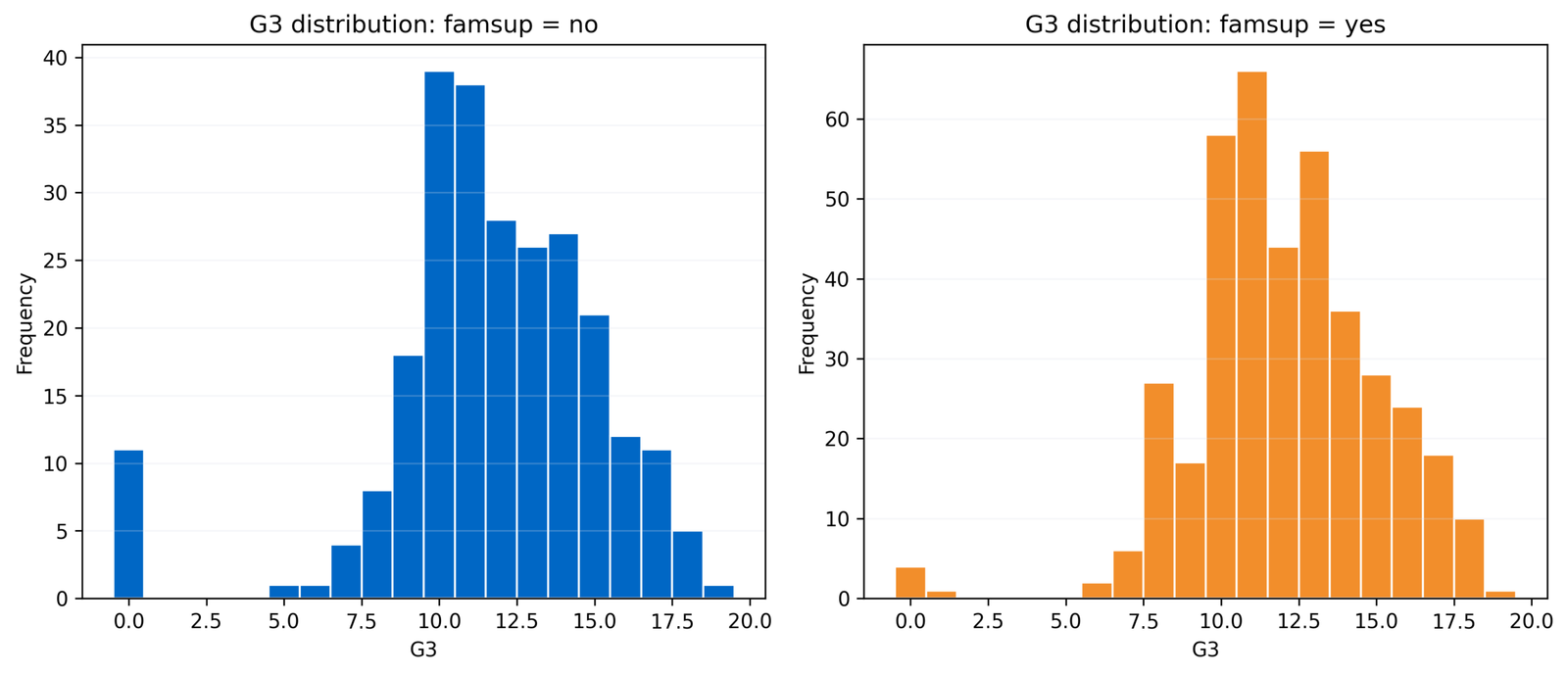
Group distributions
Both groups are centered near 12, while the no-support group has a somewhat larger standard deviation. The shape comparison should be read alongside the boxplot and ECDF rather than treated as a stand-alone significance test.
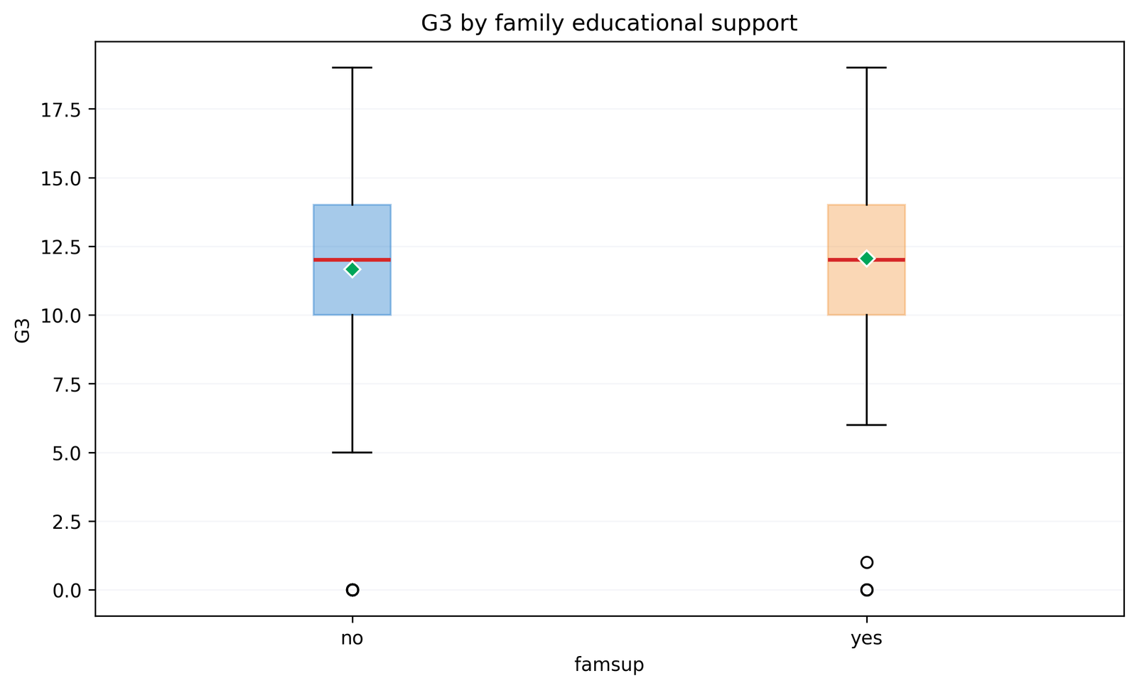
Boxplot comparison
The common median and equal IQR are visible, while tail behavior and low-grade observations explain why the standard deviations are not identical. See the guide to box plot interpretation.
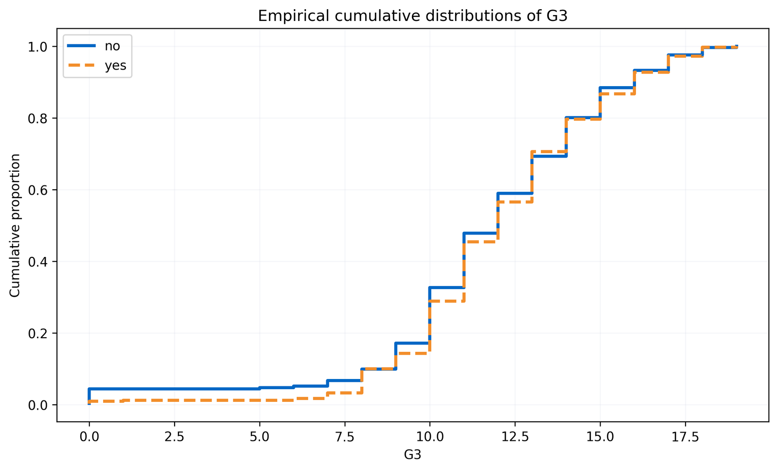
Empirical cumulative distributions
The ECDFs show the entire ordered distributions. Their proximity around the center supports the common-location description, while small tail separations are not strong enough to produce a significant scale result.
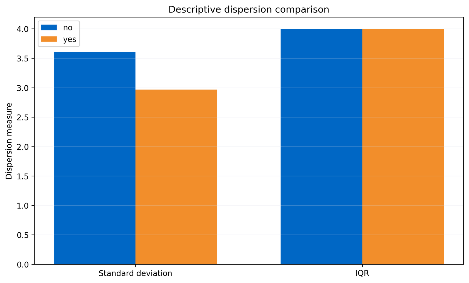
Dispersion summaries
The no-support SD is 3.602 and the support SD is 2.967, but both IQRs equal 4. This mixed descriptive picture is exactly why a rank-based scale test and visual diagnostics should be reported together.
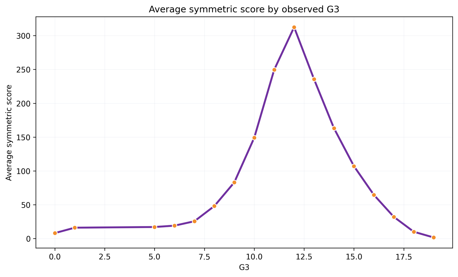
Symmetric score mechanism
Observations near the pooled center receive larger scores, and observations in the pooled extremes receive smaller scores. This chart makes the test statistic more interpretable than presenting A alone.
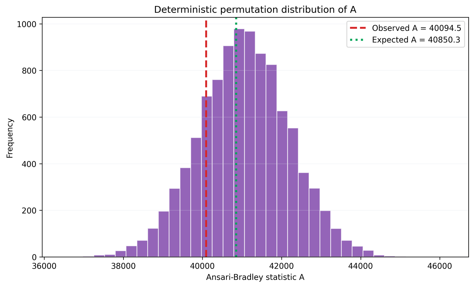
Permutation reference distribution
The observed A = 40,094.5 lies reasonably close to the null expectation of 40,850.3. Its position is not extreme, producing a two-sided permutation p-value of approximately 0.511.
Ansari Bradley test in R: ansari.test(), ties and permutation check
Base R includes ansari.test() for two-sample scale inference.
The Ansari Bradley test in R is available through ansari.test(). The R workflow below also reproduces the descriptive evidence, documents when an exact calculation is unavailable, and compares the asymptotic result with the supplied deterministic permutation result.
df <- read.csv("dataset.csv")x <- df$G3[df$famsup == "no"]
y <- df$G3[df$famsup == "yes"]
fit <- ansari.test(
x, y,
alternative = "two.sided",
exact = FALSE
)
fit
The formula interface is also convenient: ansari.test(G3 ~ famsup, data = df, exact = FALSE). For tied observations, report the approximation or a tie-capable conditional/permutation implementation and explain the method used.
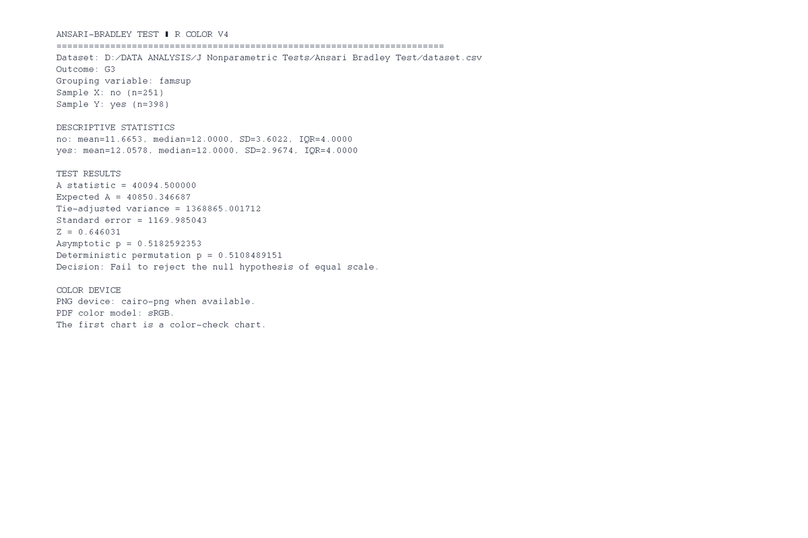
R analysis report
The R color report reproduces the Python figures exactly: n = 251 and 398, common median = 12, A = 40,094.50, |z| = 0.646, asymptotic p = 0.5183 and permutation p = 0.5108.
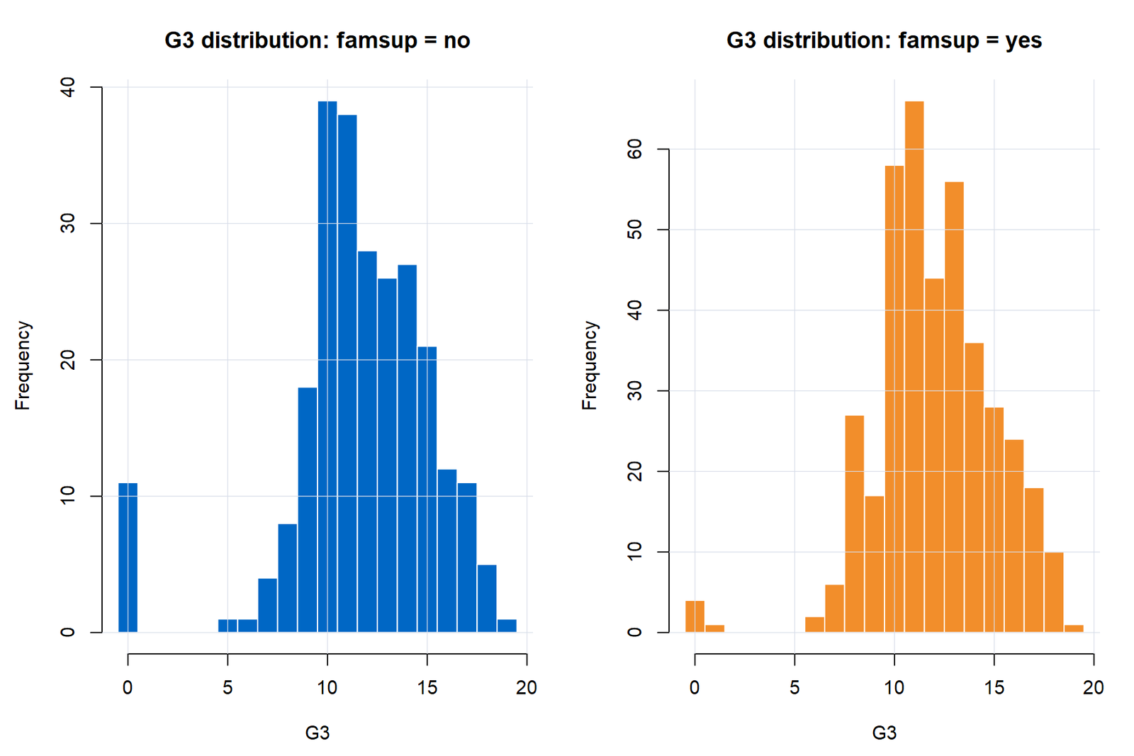
R distribution view
Separate histograms preserve the actual frequency structure of the integer-grade outcome and avoid hiding group-specific tails.
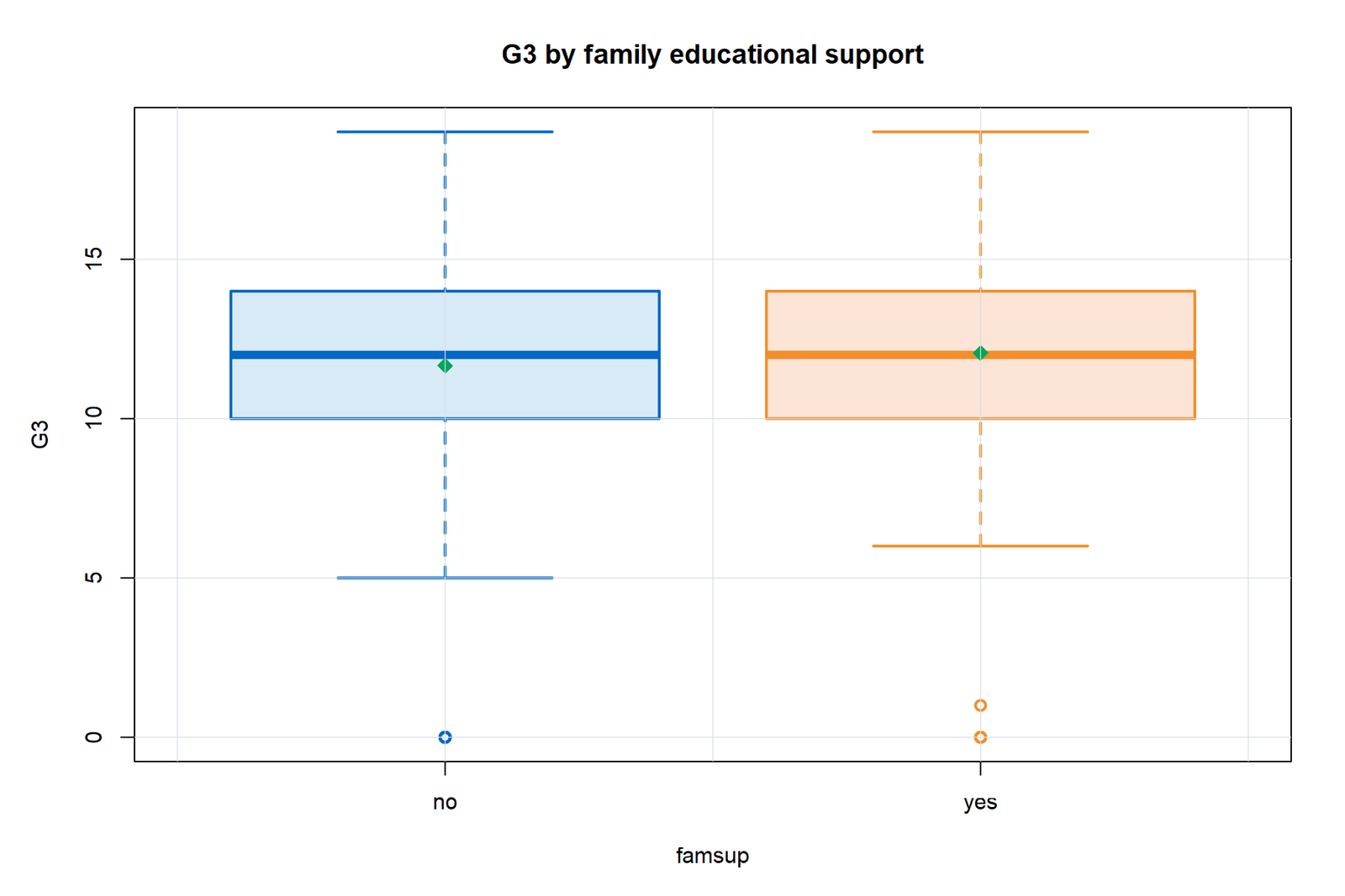
R boxplot
The medians and IQRs are aligned, while the no-support group shows greater total spread through its tail pattern.
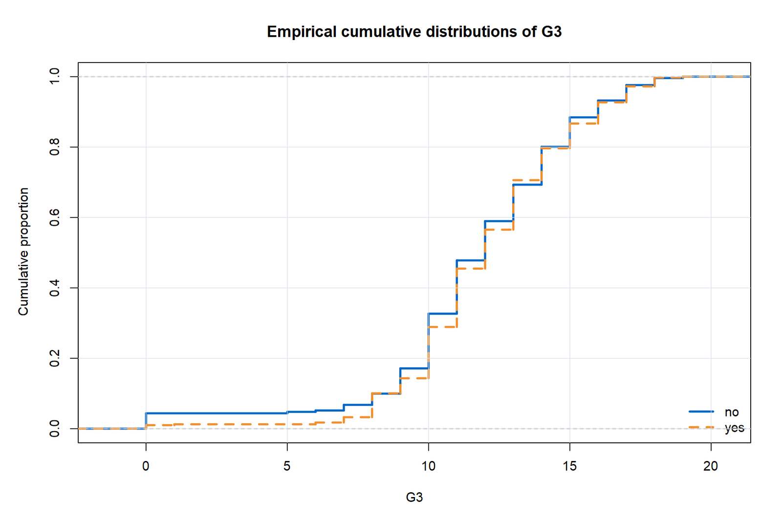
R ECDF
The cumulative curves make location, tail and crossing behavior visible without relying on histogram bin choices.
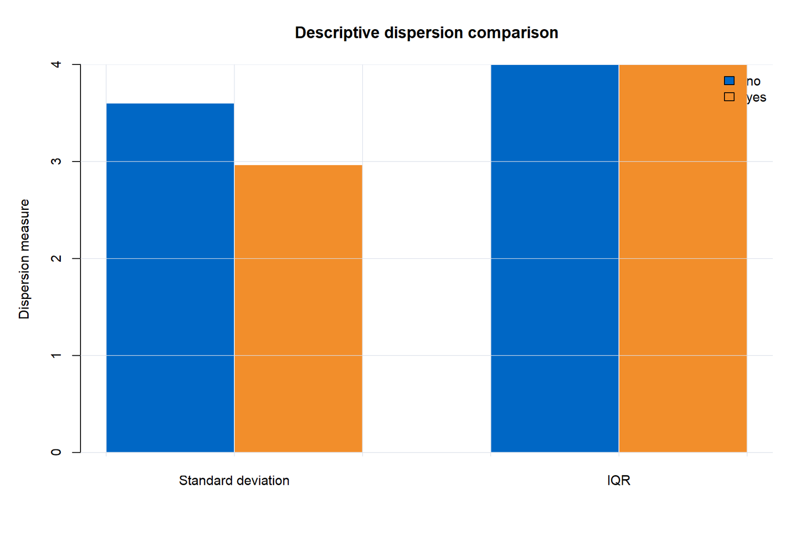
R dispersion measures
Standard deviation suggests some numerical spread difference, whereas IQR does not. The inferential test indicates that the observed difference is not statistically compelling.
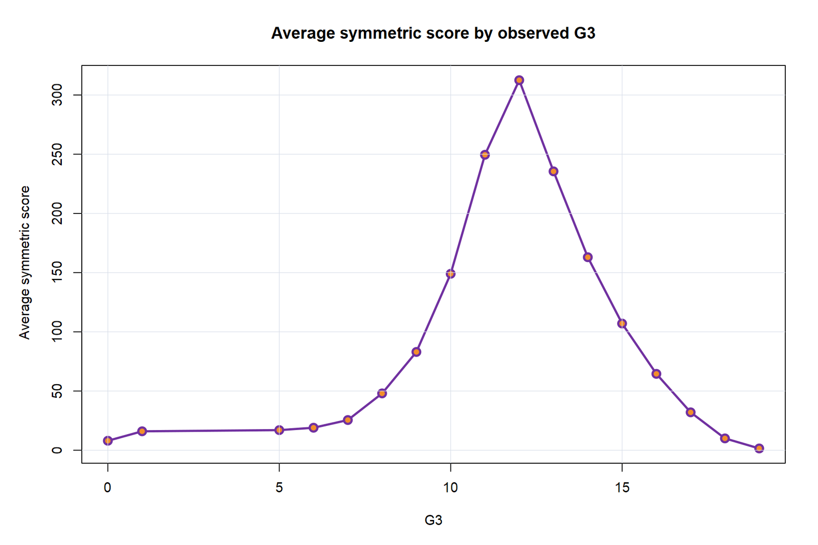
R score profile
This is the most method-specific diagnostic: it shows how observed grade values translate into center-weighted symmetric scores.
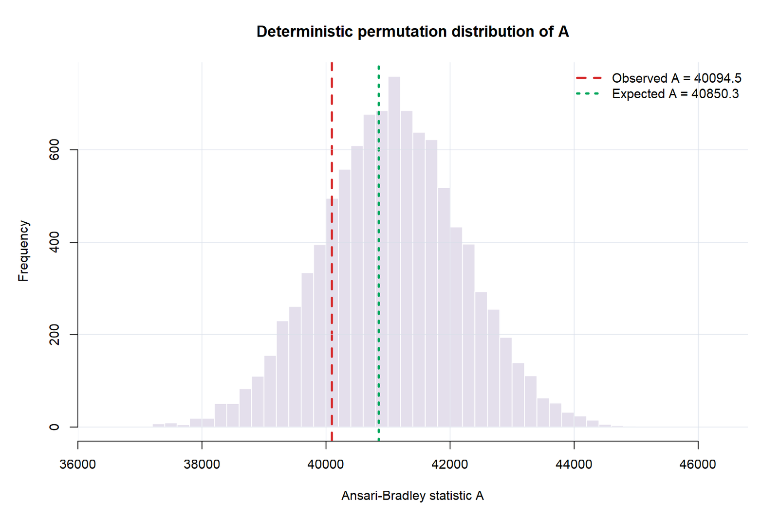
R permutation distribution
The observed statistic falls in a central region of the null distribution, matching the nonsignificant permutation result.
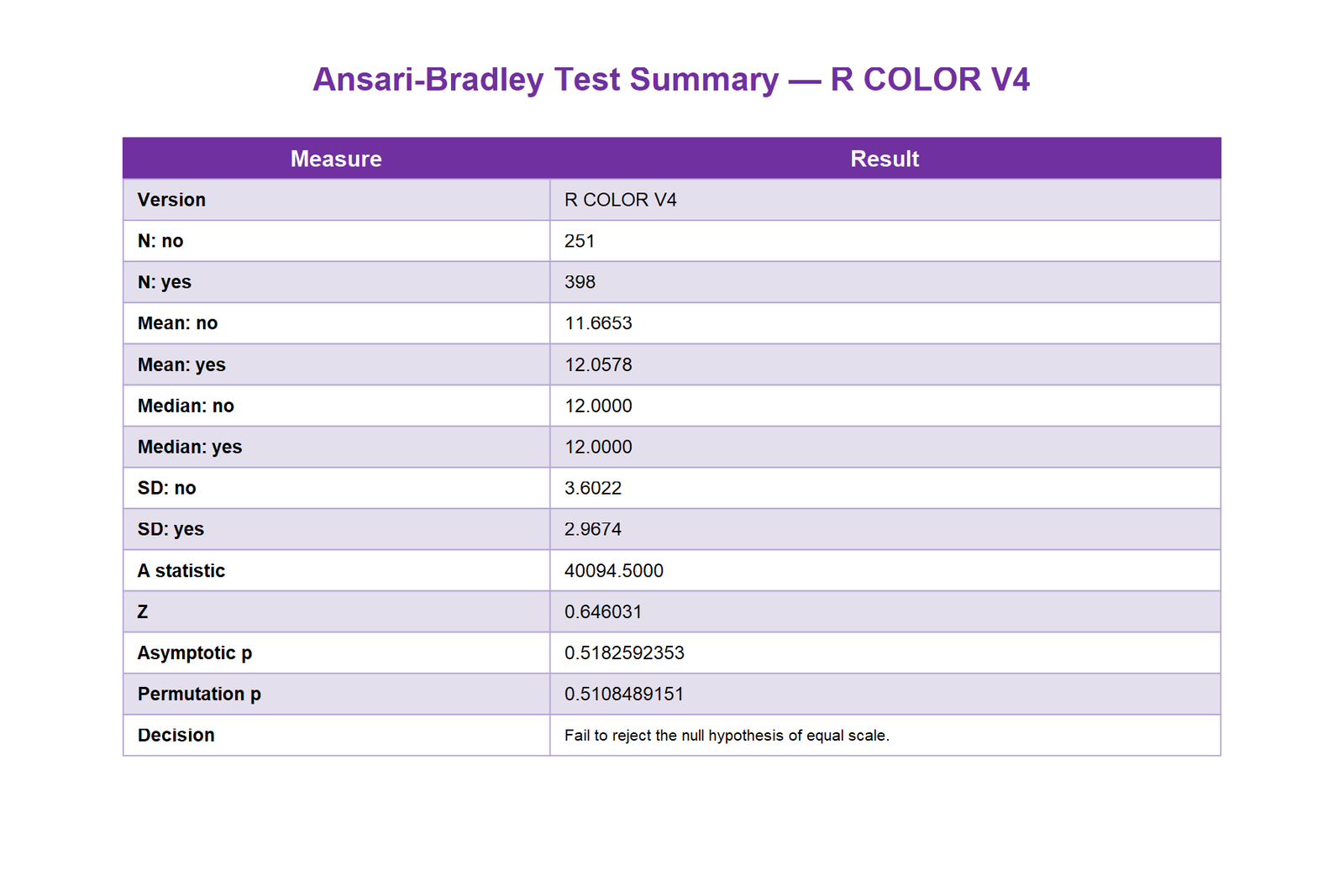
R final summary table
The final table gives a compact audit trail for reporting and confirms that the R and Python pipelines are numerically consistent.
Ansari Bradley test SPSS workflow and corrected output
SPSS is useful for data management, descriptives and charts, but the dedicated test usually requires custom computation or integrated Python/R.
An Ansari Bradley test SPSS analysis requires care because a standard menu may not expose the complete custom scoring and tie-adjusted audit used here. The corrected workflow therefore combines verified descriptives, charts and a transparent custom calculation rather than labeling a different nonparametric test as Ansari Bradley.
What the supplied SPSS output contains
The corrected report verifies 649 valid cases, produces group descriptives, histograms and a boxplot, and appends the custom Ansari-Bradley calculation. The result block reports A = 40,094.50, expected A = 40,850.35, tie-adjusted variance = 1,368,865.00, |z| = 0.646, asymptotic p = 0.5183 and permutation p = 0.5108.
The output is valuable because it separates the familiar SPSS descriptive workflow from the custom rank-score inference rather than pretending that the standard menu provides a dedicated Ansari-Bradley dialog.
Recommended SPSS workflow
EXAMINE VARIABLES=G3 BY famsup

/PLOT=BOXPLOT HISTOGRAM

/COMPARE=GROUP

/STATISTICS=DESCRIPTIVES

/CINTERVAL=95

/MISSING=LISTWISE.Ansari Bradley test Excel calculation with tie-adjusted scores
A transparent worksheet can reproduce the score sum and large-sample p-value, including tie averaging.
The Ansari Bradley test Excel worksheet is a worked calculation, not a decorative output file. It pools all 649 observations, assigns center-outward scores, averages scores within tied value blocks, sums scores for the first group and calculates E(A), Var(A), z and the two-sided probability.
Recommended worksheet structure
| Column | Contents | Example formula or action |
|---|---|---|
| A | Pooled outcome, sorted ascending | Append both samples and sort by G3. |
| B | Group label | no or yes. |
| C | Ordered position | =ROW()-1 if data begin in row 2. |
| D | Raw symmetric score | =MIN(C2,$H$1+1-C2), where H1 contains N. |
| E | Tie-adjusted score | =AVERAGEIFS($D$2:$D$650,$A$2:$A$650,A2) |
| H2 | A statistic for sample X | =SUMIFS($E$2:$E$650,$B$2:$B$650,"no") |
| H3 | Expected A | =COUNTIF($B$2:$B$650,"no")*AVERAGE($E$2:$E$650) |
| H4 | Tie-adjusted variance | =m*n/(N*(N-1))*DEVSQ($E$2:$E$650) |
| H5 | |z| | =ABS((H2-H3)/SQRT(H4)) |
| H6 | Two-sided p-value | =2*(1-NORM.S.DIST(H5,TRUE)) |
RANK.AVG and then applying a single symmetric-score formula can be wrong when a tie spans the pooled center.Ansari Bradley test in MATLAB and SAS
Equivalent commands for readers whose software search intent is not Python, R, SPSS or Excel.
The keyword set also includes Ansari Bradley test MATLAB and Ansari Bradley test SAS. These implementations should use the same group order and the same common-location interpretation as the worked analysis; a matching command name does not remove the need to check assumptions.
MATLAB
x = G3(famsup == "no");

y = G3(famsup == "yes");

[h,p,stats] = ansaribradley(x,y,'Tail','both');
Report p, the decision h, the group order and the statistic structure. With the current data, the expected conclusion is nonrejection at α = .05. Exact numeric equality across packages can depend on tie handling and approximation details, so the method field should be stated.
SAS
proc npar1way data=student ab;

class famsup;

var G3;

exact ab;

run;
The AB option requests analysis based on Ansari Bradley scores. For a large tied dataset, inspect whether the requested exact method is feasible and report the asymptotic analysis when that is the method actually produced. Do not substitute the Wilcoxon location test for this scale test.
Siegel-Tukey vs Ansari Bradley test and other dispersion tests
Choose the test that matches the design, null hypothesis and distributional conditions.
The Siegel-Tukey vs Ansari Bradley test decision is less important than choosing the correct research target. Both are rank-based scale procedures, while Levene and Brown–Forsythe test transformed deviations, Bartlett and the F test rely more heavily on normal-theory variance logic, and Fligner–Killeen extends robust dispersion testing beyond two groups.
| Method | Main question | Key conditions | Best use | Main caution |
|---|---|---|---|---|
| Ansari-Bradley | Equal scale for two independent populations? | Common location; comparable shape; ordered outcome. | Two-sample nonparametric scale comparison. | Median differences can invalidate the scale interpretation. |
| Siegel-Tukey | Do two samples differ in spread? | Independent samples; common location for a pure spread interpretation. | Alternative rank-score dispersion test. | Different score ordering; ties and location shifts need care. |
| Levene test | Equal variances based on absolute deviations? | Independent groups; less normality-sensitive than Bartlett. | Common practical homogeneity-of-variance analysis. | Still targets a different statistic and null construction. |
| Brown-Forsythe | Equal spread using median-centered absolute deviations? | Independent groups. | Robust variance homogeneity testing. | Not a symmetric-rank scale test. |
| Bartlett test | Equal variances under normality? | Independent normal populations. | High power when normality is credible. | Very sensitive to non-normality. |
| F test | Is the ratio of two normal-population variances equal to 1? | Independent normal samples. | Classical two-group variance comparison. | Can be unreliable under non-normality. |
| Fligner-Killeen | Equal dispersion across two or more groups? | Independent groups; rank-based. | Robust k-sample homogeneity analysis. | Different scoring and interpretation from Ansari-Bradley. |
Diagnostics, sensitivity checks and common mistakes
A defensible analysis combines the p-value with design and distribution checks.
A credible Ansari Bradley test report must show that a nonsignificant p-value is not being mistaken for proof of identical variability. Diagnostics should examine group centers, shapes, ties, bounded outcomes, influential tail patterns, sample imbalance and whether the chosen scale estimand matches the research question.
Before the test
After the test
Frequent reporting errors
| Error | Why it is wrong | Better practice |
|---|---|---|
| Calling it a test of medians | The statistic is designed for scale differences. | Describe the population scale or dispersion hypothesis. |
| Ignoring unequal medians | Location shifts can alter symmetric scores and create misleading evidence. | Assess and justify common location before testing. |
| Reporting only SDs | SDs can differ numerically without a significant population-scale result. | Report medians, IQRs, SDs, visuals, A and p-values. |
| Using exact language with ties | Exact null distributions usually require special handling when tied values occur. | State whether inference is asymptotic, conditional or permutation-based. |
| Equating p > .05 with equivalence | Failure to reject is not evidence within a prespecified equivalence margin. | Use cautious language or design a formal equivalence analysis. |
Review outlier detection and descriptive statistics for the visual and numerical checks that should accompany the test.
How to report the Ansari Bradley test in APA style
Include the scale question, group summaries, inference method and cautious conclusion.
Report the Ansari Bradley test with the group definitions, sample sizes, common-location evidence, statistic, reference method, p-value, direction convention and a restrained conclusion. Do not write “the variances are equal” merely because p exceeds .05.
APA-style result
Compact technical report
Ansari-Bradley: A = 40,094.50; E(A) = 40,850.35; tie-adjusted SE = 1,169.99; |z| = 0.646; asymptotic p = .5183; permutation p = .5108; two-sided α = .05; fail to reject equal scale.
Reporting checklist
Ansari Bradley test PDF, Excel and software downloads
Open the exact analysis reports and the worked Excel workbook.
The downloadable Ansari Bradley test PDF reports and worked Excel file allow readers to verify every numerical result. The Python, R, corrected SPSS and Excel outputs all refer to the same G3-by-famsup analysis and should agree before publication.
R reportColor R analysis with matched results and all diagnostic charts.Open R PDF →
SPSS reportCorrected SPSS descriptives, charts and custom Ansari-Bradley result block.Open SPSS PDF →
Worked Excel fileTransparent pooled ranking, tie-adjusted scores, statistic, z and p-value calculations.Download Excel →
Official Ansari Bradley test references and software documentation
Authoritative documentation used to verify the scoring rule, software syntax and interpretation.
The Ansari Bradley test implementation and terminology in this guide were checked against primary technical documentation rather than copied from short competitor summaries. These sources also help readers verify software behavior when ties, exact probabilities or one-sided alternatives are involved.
SciPy documentation
The official SciPy scipy.stats.ansari documentation defines the Python function, alternatives and returned statistic.
R documentation
The official R stats::ansari.test documentation explains the formula interface, exact calculation, confidence interval and treatment of ties.
NIST score reference
The NIST Ansari-Bradley score reference documents the symmetric score sequence used by the test.
Ansari Bradley test FAQs
Answers to the questions most often missed in short competitor explanations.
These Ansari Bradley test FAQs answer the search questions most often missed by brief definitions: what the test measures, why equal medians matter, how ties change the calculation, when the large-sample approximation is used, how R and Python label one-sided alternatives, and how it differs from the Siegel–Tukey test.
What is the Ansari Bradley test?
Is the Ansari Bradley test a test of variances?
What are the Ansari Bradley test assumptions?
Why must the medians be equal for the Ansari Bradley test?
Can I subtract each sample median before the Ansari Bradley test?
How do ties affect the Ansari Bradley test?
What is the difference between the Ansari Bradley test and Siegel-Tukey?
What is the large-sample Ansari Bradley test?
How do I interpret a significant Ansari Bradley test result?
How do I interpret p = .518 in this Ansari Bradley test example?
Can the Ansari Bradley test be used for more than two groups?
Is there a direct Ansari Bradley test menu in SPSS?
Related statistical guides
Continue with the methods and interpretation concepts most closely connected to scale testing.