
Mood’s Median Test: Formula, Interpretation, Python, R, SPSS and Excel Guide
The Mood’s Median Test is a robust nonparametric procedure for comparing the medians of three or more independent groups. This complete guide explains what the Mood’s Median Test measures, when to use it, how the pooled-median contingency table is constructed, how the chi-square statistic is calculated, and how a four-group worked example can be interpreted in Python, R, SPSS, and Excel.
Pooled median = 12
Chi-square on above/below counts
Python + R + SPSS + Excel
Full worked example
Mood’s Median Test found a statistically significant difference in final-grade medians across the four school-choice reason groups.
In this worked Mood’s Median Test example, the outcome variable is G3 and the grouping variable is reason, with categories course, home, other, and reputation. One pooled median of 12 is calculated from all 649 final-grade observations. Each observation is then classified as above the pooled median or at or below the pooled median. The resulting 4 × 2 contingency table produces χ²(3) = 22.6682 with p = 0.00004735. The null hypothesis that all four groups share the same population median is therefore rejected.
What does Mood’s Median Test measure?
A direct, robust comparison of median location across independent groups using one pooled center.
The Mood’s Median Test, sometimes written as Mood median test, Mood’s k-sample median test, or simply k-sample median test, evaluates whether several independent populations share the same median. It is one of the most transparent nonparametric procedures because its logic can be explained without complicated rank formulas. The method calculates one median from the combined sample, classifies every observation relative to that pooled center, and then uses a chi-square statistic to test whether the above-versus-below pattern is independent of group membership.
This pooled-center design gives the Mood’s Median Test a distinctive identity. Unlike a mean-based ANOVA, it does not model group means. Unlike a full-rank method, it does not retain the exact rank position of every observation. Instead, it asks a narrower and highly interpretable question: does each group contribute the same proportion of observations above the pooled median? If the proportions differ more than sampling variation would reasonably explain, the test rejects the equal-median null hypothesis.
Why the method remains useful
The Mood’s Median Test remains useful because the median is a robust measure of center. It is less sensitive to unusually low or high observations than the mean, which makes it attractive for skewed, bounded, or heavy-tailed data. The method is also easy to audit: anyone can inspect the pooled median, the classification rule, the observed table, and the expected counts.
That transparency connects the method naturally to the Pearson Chi-Square Test, the G-Test, and the Likelihood Ratio Chi-Square. The inferential engine is table-based, but the table itself is created from a median-focused transformation of a numeric outcome.
What information the test deliberately discards
The simplicity of the Mood’s Median Test comes from collapsing the outcome into only two categories: above the pooled median and at/below the pooled median. A score of 13 and a score of 19 receive the same classification, even though their raw values differ substantially. Likewise, two observations below the median may be far apart on the original scale but still enter the same table cell.
This means the method can be less statistically powerful than procedures that retain more of the ordering information. That limitation does not make the test invalid; it simply means the Mood’s Median Test is best chosen when the median itself is the central scientific target and interpretive simplicity is valuable.
The method is especially helpful in public-facing educational content because readers can visualize the logic. They do not have to accept a black-box statistic. They can see the pooled median of 12, count how many observations in each reason group lie above that threshold, and compare those observed numbers with the counts expected under equal medians.
It also provides a useful conceptual bridge between nonparametric location testing and categorical-data analysis. Readers familiar with a Sign Test understand the idea of reducing data to directional categories. Readers familiar with chi-square testing understand observed-versus-expected counts. The Mood’s Median Test combines those two intuitions in one coherent method.
For the current dataset, the four groups are not arbitrary labels. They represent different stated reasons for school choice: course, home, other, and reputation. The test therefore asks whether the typical final-grade position differs across those four reason categories. Because the response is a final grade and the groups are independent, a median-centered comparison is easy to justify and easy to communicate.
When should you use Mood’s Median Test?
Choose it when several independent groups must be compared specifically on median location.
Common searches include when to use Mood’s median test, what is Mood median test, and how to interpret Mood’s median test. The practical decision rule is straightforward: use the Mood’s Median Test when you have two or more independent groups, an outcome that supports a meaningful median, and a research question focused specifically on whether the population medians differ.
Independent groups
Each observation belongs to one group only. Here, every student belongs to one school-choice reason category.
Rankable or numeric outcome
The outcome must support ordering and a meaningful pooled median. Final grade G3 satisfies that condition.
Median-focused question
The method is most appropriate when the central inferential target is the median rather than the mean or full rank distribution.
Robust preference
The test is attractive when skewness, repeated values, or outliers make a resistant center desirable.
Readable public explanation
Observed and expected counts provide a very accessible way to communicate the result.
Situations that fit the method well
Situations where another method may fit better
Another reason to use the Mood’s Median Test is that it can accommodate unequal group sizes naturally. The four groups in the worked example range from 72 observations in the other category to 285 observations in the course category. Expected counts automatically incorporate those different row totals, so the test does not require balanced groups.
The method also handles tied values through a declared classification rule. In the current workbook, observations equal to the pooled median are classified as at or below. That rule should be stated in the public article because it affects the table counts. Clear tie handling is not a minor technicality; it is part of the definition of the analysis.
For readers choosing among nonparametric methods, it helps to ask whether the goal is to detect any distributional difference or specifically a median difference. Procedures such as the Ansari-Bradley Test target scale, while the Mood’s Median Test targets center. A Dunn’s Test or Conover Test is usually a post hoc procedure after an omnibus result. These methods are related, but they answer different questions.
That method-selection discipline is important. Nonparametric does not mean interchangeable. A good analysis begins with the research question and chooses the procedure whose statistical target matches that question. When the question is “Do these independent groups share the same median?”, the Mood’s Median Test is one of the clearest direct answers.
Mood’s Median Test assumptions
The procedure is robust and nonparametric, but it still depends on a valid independent-group design.
The Mood median test assumptions are lighter than many parametric assumptions, but they must still be checked. The groups should be independent, the outcome should have a meaningful order and median, one pooled median must be calculated before group classification, the tie rule must be consistent, and the expected cell counts should be adequate for the chi-square approximation.
Independent observations
Each student belongs to one reason category only. No observation is repeated across course, home, other, and reputation groups.
Meaningful pooled center
G3 is a numeric final-grade score, so the pooled median of 12 has a clear and interpretable meaning.
One common median
The pooled median is calculated from all 649 observations together, not by averaging the four group medians.
Consistent tie rule
Scores equal to 12 are placed in the at-or-below category. This rule is applied identically in every reason group.
Adequate expected counts
The smallest expected frequency is 30.6194, so every cell is comfortably large for the chi-square reference.
Correct target of inference
The safest conclusion is about median equality and the pooled-median classification, not about every distributional feature.
Independence is the most important design requirement. If the same students were observed repeatedly under different conditions, the above/below counts would not form independent rows, and a repeated-measures method such as the Friedman Test would be more appropriate. The current reason groups are separate, so the independent-design assumption is satisfied.
The expected-count condition is also easy to verify. Course has expected counts of 121.2018 above and 163.7982 at/below. Home has expected counts of 63.3652 and 85.6348. Other has 30.6194 and 41.3806. Reputation has 60.8136 and 82.1864. None of these values is remotely small, so the chi-square approximation is well supported.
The method does not require normality. That is one of its main attractions. Final-grade distributions can contain repeated values, limited ranges, and unusual shapes, yet the pooled-median framework remains valid so long as the design and classification assumptions are respected.
Readers should also distinguish “same median” from “identical distributions.” Two groups could share a median but differ in spread or tail behavior. Conversely, a significant Mood’s Median Test indicates a difference in the median-centered classification pattern, but it does not describe every way the distributions differ. Keeping that distinction clear improves methodological accuracy.
Null and alternative hypotheses
The hypotheses are global because the test compares all four independent groups at once.
Null hypothesis
H0: the course, home, other, and reputation populations share the same median final grade.
Equivalently, after fixing the pooled median at 12, the probability of falling above that median is the same in every reason group.
Alternative hypothesis
H1: at least one reason group has a different population median.
Equivalently, the above-versus-at/below classification depends on group membership.
G3 final grade
reason with four categories
four independent samples
This is an omnibus hypothesis structure. A significant Mood’s Median Test tells us that not all medians are equal, but it does not automatically identify every pairwise difference. The observed table provides strong directional clues, yet formal pairwise follow-up would require additional procedures or adjusted comparisons.
That distinction between omnibus and pairwise inference is central to good reporting. The overall result answers the global question first. Only after that result is significant should the analyst consider targeted follow-up comparisons. This sequencing protects the interpretation from becoming a collection of unplanned pairwise claims.
The hypothesis framework is especially intuitive when expressed through probabilities. Under the null, the overall above-median proportion of 42.53% should apply equally to every group after accounting for sample size. Under the alternative, some groups will exceed that rate and others will fall below it. The observed proportions—36.49%, 48.99%, 27.78%, and 55.24%—show exactly that kind of divergence.
For public readers, the phrase “at least one group differs” is important. It prevents the common mistake of interpreting a global p-value as proof that every pair differs from every other pair. Mood’s test establishes that the four-group median pattern is not uniform; the detailed count table then helps explain where the largest deviations occur.
Mood’s Median Test formula and calculation logic
The method uses a Pearson chi-square statistic applied to the k × 2 pooled-median table.
For every reason-by-classification cell, the observed count O is compared with the expected count E. The eight cell contributions are added to produce the final Mood’s Median Test statistic.
The expected frequency for each cell equals its reason-group total multiplied by the above/below column total, divided by the complete sample size of 649.
With four reason groups, the table has 3 degrees of freedom. The observed chi-square statistic is compared with the chi-square distribution using df = 3.
For a 4 × 2 table, the smaller dimension minus one equals 1, so Cramér’s V reduces to √(χ²/N). The derived value for this example is 0.1869.
The calculation begins with the pooled median. Across all 649 G3 scores, the median is 12. Values greater than 12 are classified as above median. Values equal to or below 12 are classified as at/below. This produces 276 above-median observations and 373 at/below observations across the full sample.
Under the null hypothesis, every group should have an above-median rate close to the overall rate of 276/649 = 42.53%. Expected counts implement that idea while respecting each group’s sample size. The course group has 285 observations, so its expected above count is 285 × 276 / 649 = 121.2018. The reputation group has 143 observations, so its expected above count is 60.8136.
Exact calculation components
Largest cell contributions
The reputation-above cell contributes 5.4387 to chi-square because 79 observations are above the median compared with only 60.8136 expected. The reputation-at/below cell contributes 4.0243. The other-above cell contributes 3.6830 because only 20 observations are above median compared with 30.6194 expected.
Those three cells explain much of the result. Reputation is substantially higher than the null pattern, while other is substantially lower. Course also contributes in the lower direction, and home contributes moderately in the higher direction.
The formula therefore tells a very readable story. The test is significant not because of one mysterious software decision, but because the observed table contains systematic departures from the equal-median expectation. Every contribution can be traced to a specific group and classification cell.
This auditability is a major strength of Mood’s Median Test. A reader can verify the pooled center, the row totals, the column totals, the expected counts, and the individual chi-square contributions. That makes the procedure especially suitable for Excel-based teaching and public statistical reporting.
Variables and data dictionary
The worked example compares final grades across four school-choice reason categories.
| Variable | Role | Description |
|---|---|---|
| G3 | Outcome variable | Final-grade score used to calculate the pooled median and classify observations. |
| reason | Grouping variable | Independent school-choice reason with four categories. |
| course | Group 1 | Students choosing the school primarily for the course; n = 285. |
| home | Group 2 | Students choosing the school because it is close to home; n = 149. |
| other | Group 3 | Students reporting another school-choice reason; n = 72. |
| reputation | Group 4 | Students choosing the school for its reputation; n = 143. |
| Above median | Derived classification | G3 strictly greater than 12. |
| At or below | Derived classification | G3 equal to or less than 12. |
The descriptive medians already suggest the omnibus result. Course and other each have a median of 11, home has a median of 12, and reputation has a median of 13. The pooled median of 12 lies between the lower-center and higher-center groups, so the above/below classification naturally separates reputation and other most strongly.
The mean values tell a similar story. Reputation has the highest mean at 12.9441, followed by home at 12.1812, course at 11.5474, and other at 10.6944. Although Mood’s Median Test does not test means, this alignment between mean and median summaries makes the direction of the result easier to understand.
The group sizes are unequal, but that is not a problem. Expected counts are based on each row total, so the larger course group receives larger expected counts than the smaller other group. The comparison is therefore about proportions relative to the pooled median, not raw counts alone.
A clear data dictionary prevents software output from becoming anonymous. Naming G3, reason, and the four categories explicitly makes the public explanation more meaningful and ensures that every statistic can be connected back to the actual research design.
Worked example: final grades across school-choice reasons
The four-group example reveals how different reason categories contribute to the pooled-median result.
This Mood’s Median Test example begins with 649 student records. The pooled median of G3 is 12. Every score greater than 12 is classified as above median, and every score equal to or below 12 is classified as at/below. The four reason groups then contribute different observed count patterns.
The course group contains 104 above-median and 181 at/below observations. That above-median rate is 36.49%, below the overall rate of 42.53%. The home group contains 73 above and 76 at/below, producing a rate of 48.99%. The other group contains only 20 above and 52 at/below, a rate of 27.78%. Reputation contains 79 above and 64 at/below, the highest rate at 55.24%.
Observed proportions above the pooled median
| Reason | Above / n | Above-median percentage | Direction versus overall rate |
|---|---|---|---|
| course | 104 / 285 | 36.49% | Below 42.53% |
| home | 73 / 149 | 48.99% | Above 42.53% |
| other | 20 / 72 | 27.78% | Well below 42.53% |
| reputation | 79 / 143 | 55.24% | Well above 42.53% |
Observed omnibus result
The table differences produce a statistically significant four-group median comparison.
The equal-median null is rejected. Reputation shows the strongest high-center pattern, while other shows the strongest low-center pattern.
The expected-count comparison clarifies why the statistic is large. Course has 17.2018 fewer above-median observations than expected. Home has 9.6348 more than expected. Other has 10.6194 fewer than expected. Reputation has 18.1864 more than expected. These deviations are not random in direction; they form a coherent pattern of lower and higher median-centered groups.
The reputation group is particularly influential. It contains 79 above-median observations compared with only 60.8136 expected, and just 64 at/below observations compared with 82.1864 expected. Together, those two cells contribute 9.4630 of the total chi-square statistic.
The other group is the second clearest contributor. It contains only 20 above-median observations compared with 30.6194 expected, and 52 at/below compared with 41.3806 expected. Those cells contribute 6.4083 to chi-square. The combined reputation-versus-other contrast therefore explains much of the global result, even though formal pairwise inference would require separate testing.
This worked example shows the educational value of Mood’s Median Test. Readers can identify the pooled center, inspect the count pattern, understand the expected counts, and see where the chi-square statistic comes from. The analysis is rigorous without becoming opaque.
Exact observed, expected, and contribution results
The full table reveals which group cells drive the significant omnibus result.
| Reason | Observed above | Observed at/below | Expected above | Expected at/below |
|---|---|---|---|---|
| course | 104 | 181 | 121.2018 | 163.7982 |
| home | 73 | 76 | 63.3652 | 85.6348 |
| other | 20 | 52 | 30.6194 | 41.3806 |
| reputation | 79 | 64 | 60.8136 | 82.1864 |
| Cell | Observed minus expected | Chi-square contribution | Interpretive role |
|---|---|---|---|
| course above | −17.2018 | 2.4414 | Fewer above-median scores than expected. |
| course at/below | +17.2018 | 1.8065 | More lower-side scores than expected. |
| home above | +9.6348 | 1.4650 | Moderately more above-median scores. |
| home at/below | −9.6348 | 1.0840 | Moderately fewer lower-side scores. |
| other above | −10.6194 | 3.6830 | Strong shortage of above-median scores. |
| other at/below | +10.6194 | 2.7252 | Strong excess of lower-side scores. |
| reputation above | +18.1864 | 5.4387 | Largest positive high-side departure. |
| reputation at/below | −18.1864 | 4.0243 | Largest shortage of lower-side scores. |
What the exact results mean
The significant Mood’s Median Test result is driven mainly by the reputation and other groups. Reputation has substantially more observations above the pooled median than expected, while other has substantially fewer. Course also tends lower than the null pattern, and home tends higher. The global result therefore reflects a meaningful and interpretable ordering of median-centered performance across the four school-choice reasons.
The final reported statistic is χ²(3) = 22.6682461965. The p-value is 0.00004735096, which is far below 0.05. The workbook cross-check shows essentially zero numerical difference between its result and the independently verified reference calculation.
The derived effect size Cramér’s V = 0.1869 provides useful scale. The association is not enormous, but it is clearly nontrivial. Statistical significance is strengthened by the large sample size, while the effect-size estimate reminds readers that the result should be interpreted as a meaningful but not overwhelming group association.
This combination of significance and effect size produces a balanced conclusion. The groups differ clearly in median-centered performance, yet school-choice reason does not explain all variation in final grades. Individual differences remain substantial within every group.
How to interpret Mood’s Median Test
A strong interpretation combines the omnibus decision, group direction, and effect-size context.
Readers searching how to interpret Mood’s median test need more than a p-value. A complete interpretation should report the pooled median, the chi-square statistic, degrees of freedom, the p-value, the direction of the group count pattern, and an effect-size statement.
Statistical decision
Because p = 0.00004735, the null hypothesis that all four groups share the same median is rejected.
Direction of the pattern
Reputation and home have above-median rates above the overall 42.53%, while course and other have rates below it.
Magnitude
Cramér’s V = 0.1869 indicates a modest but meaningful association between reason group and median classification.
The most direct public interpretation is that final-grade median patterns differ across school-choice reasons. Students in the reputation group are most likely to appear above the pooled median, followed by home. Course is lower, and other is the lowest. The descriptive medians of 13, 12, 11, and 11 support the same broad story.
Good interpretation avoids claiming that every group pair is statistically different. The omnibus Mood’s Median Test establishes that at least one median differs. The observed table strongly suggests that reputation and other are far apart, but pairwise confirmation would require additional comparisons with appropriate multiplicity control.
The result should also not be interpreted causally. Choosing a school for reputation does not necessarily cause higher grades. The reason categories may reflect other student, family, school, or contextual characteristics. The analysis establishes a robust association between reason group and median-centered grade position, not a causal mechanism.
At the same time, the finding should not be minimized. The p-value is very small, the expected counts are all adequate, and the observed pattern is coherent. Reputation is above expectation in the favorable direction, other is below expectation, and the raw descriptive summaries align with the table-based inference.
A polished interpretation can therefore state: Mood’s Median Test indicated that final-grade medians differ by school-choice reason, χ²(3) = 22.67, p < .001, Cramér’s V = .187. The reputation group showed the highest above-median proportion, whereas the other group showed the lowest.
Mood’s Median Test in Python: chart-by-chart interpretation
The Python figures explain the pooled-median result from primary metrics through group-level verification.
Searchers often want a Mood’s median test Python example that explains the result visually instead of printing only one test statistic. The chart set below keeps every image inside a complete bordered figure card with a detailed caption tied to the actual workbook results.
Python is especially useful for this method because the entire process is transparent. The pooled median can be calculated from the combined data, a binary indicator can be created with one line of logic, observed and expected tables can be generated, and each chi-square contribution can be verified. The five figures therefore form a complete learning sequence rather than a decorative image gallery.
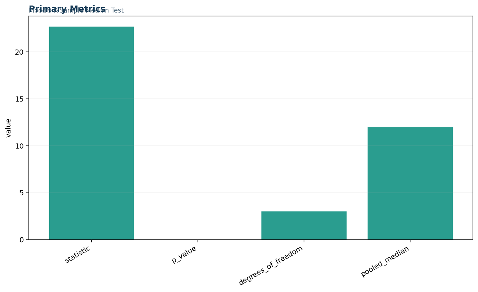
Python chart 1: primary metrics
This full-width summary chart introduces the entire result. It displays χ² = 22.6682, df = 3, p = 0.00004735, N = 649, and pooled median = 12. The figure communicates the omnibus conclusion immediately: the four reason groups do not share the same median-centered pattern.
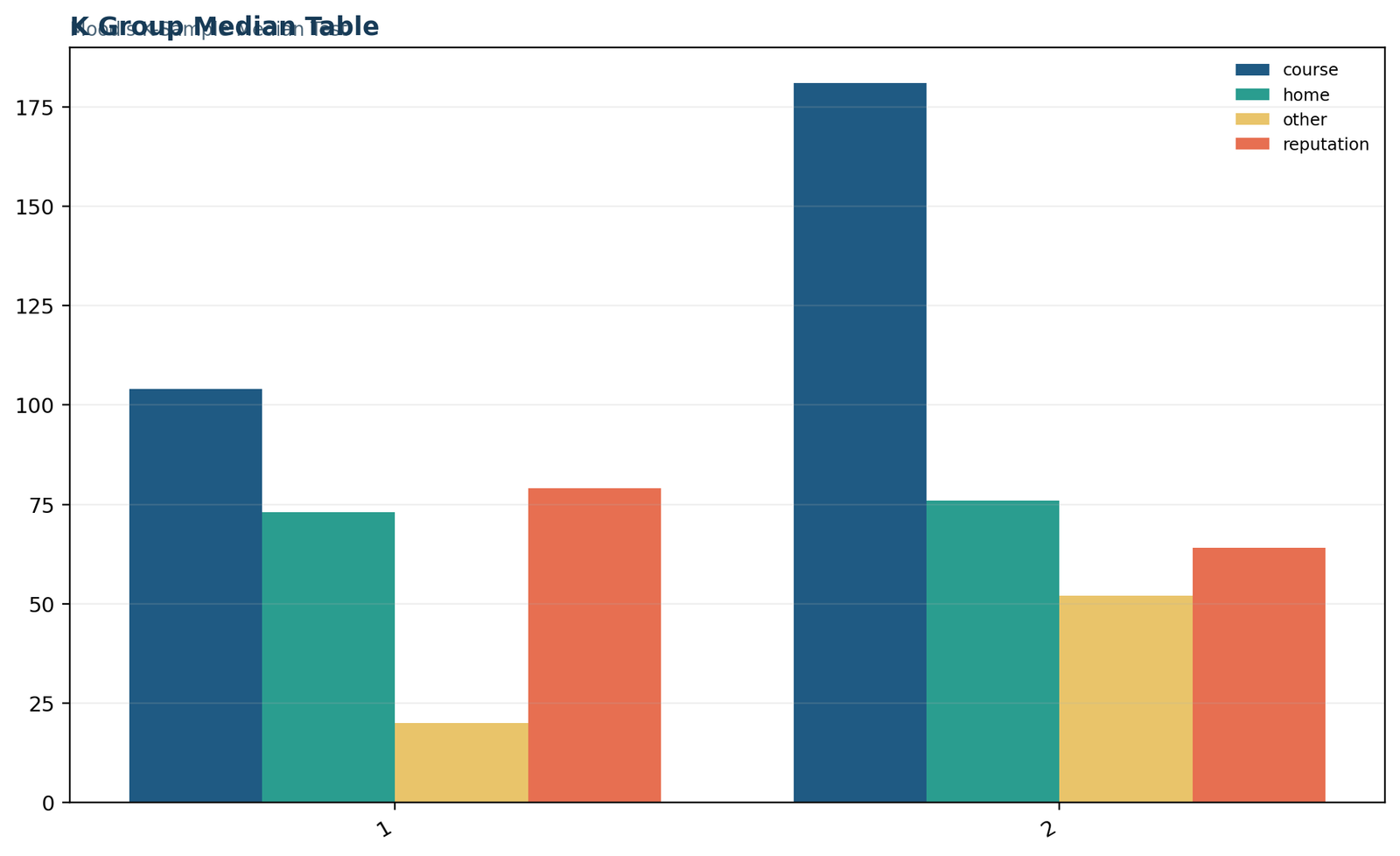
Python chart 2: k-group median table
This chart visualizes the observed 4 × 2 table. Course contains 104 above and 181 at/below observations; home contains 73 and 76; other contains 20 and 52; reputation contains 79 and 64. The reputation and other rows show the strongest contrast, which explains much of the significant omnibus result.
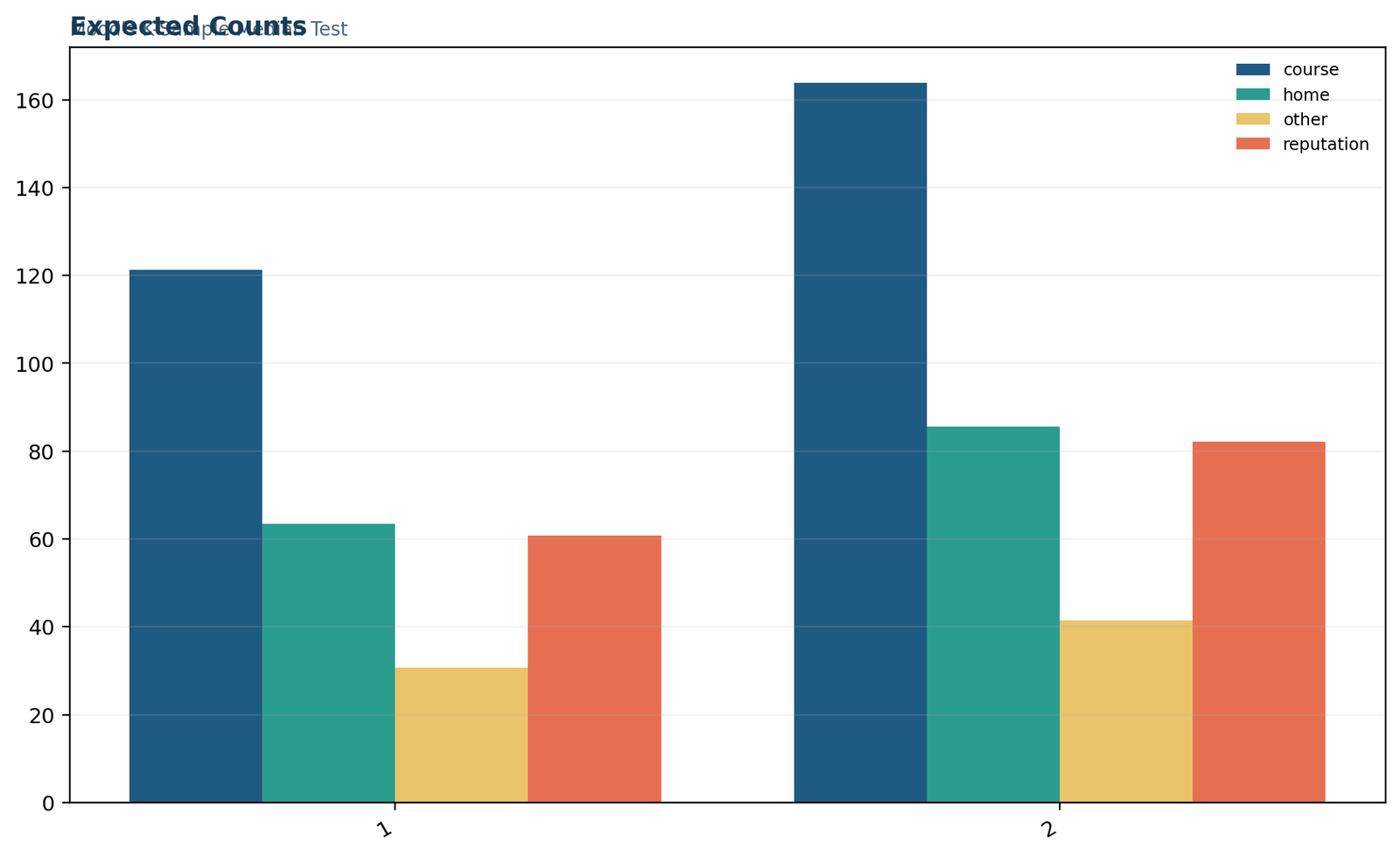
Python chart 3: expected counts
The expected-count figure shows what each group would contribute if all medians were equal. Reputation is expected to have 60.81 above-median observations but actually has 79. Other is expected to have 30.62 above but actually has only 20. This observed-versus-expected contrast is the statistical engine of the test.
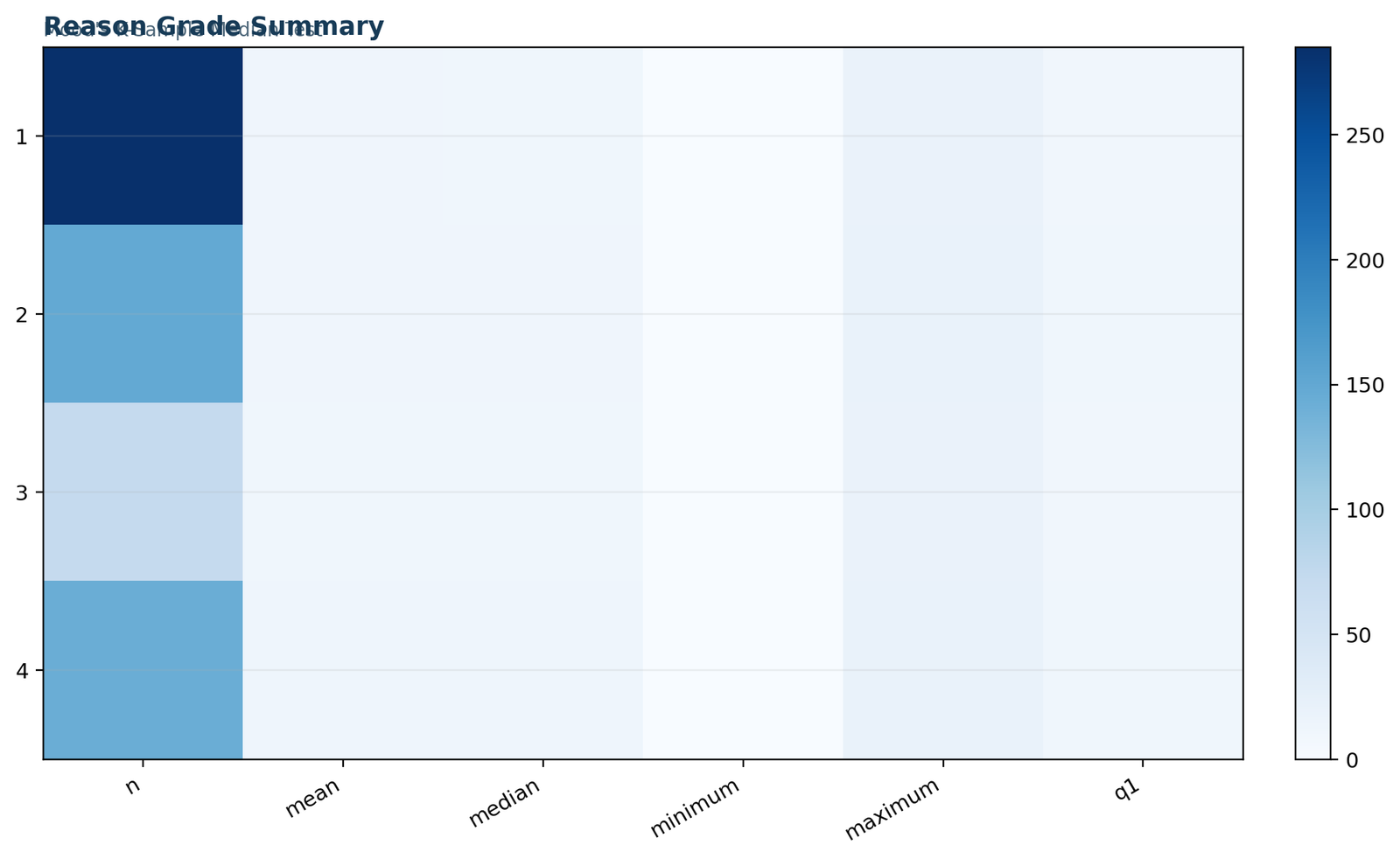
Python chart 4: reason-grade summary
This descriptive chart reconnects the table result to the original G3 scale. Reputation has the highest mean and median, home is next, while course and other are lower. The descriptive ordering supports the pooled-median count pattern and makes the result easier to interpret substantively.
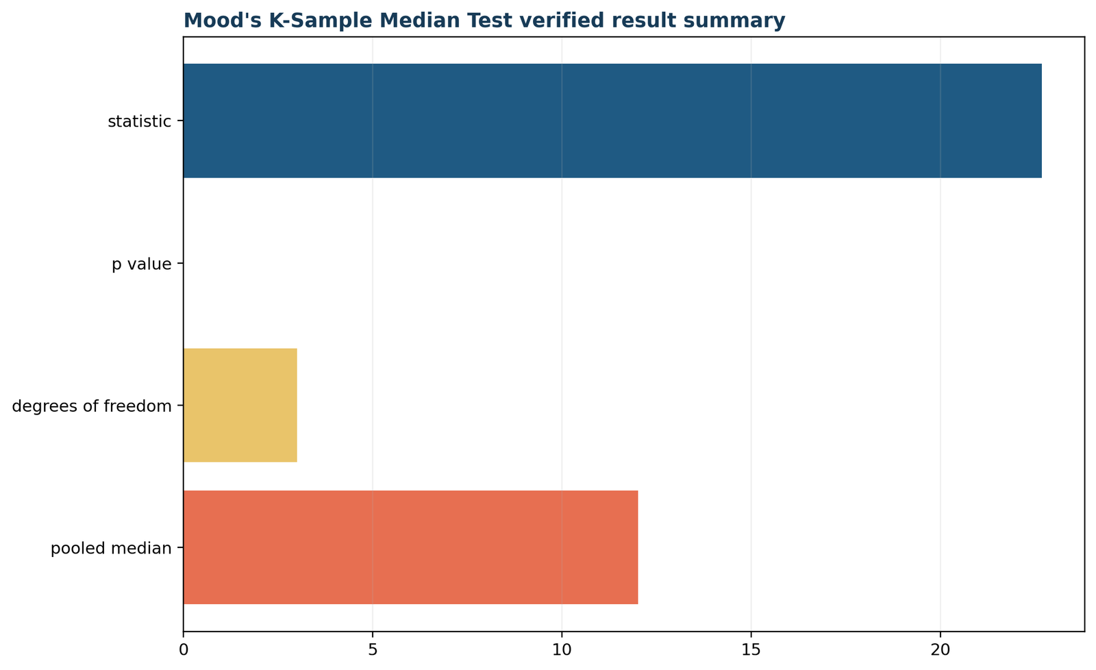
Python chart 5: verified result summary
The final Python figure condenses the complete analysis into a public-ready conclusion. The four medians are not equal, reputation shows the strongest high-center pattern, other shows the strongest low-center pattern, and the workbook values match the verified analysis.
For learners, the Python charts separate descriptive evidence from inferential evidence. The primary metrics state the result, the observed table displays the data reduction, the expected-count chart explains the chi-square calculation, the reason summary shows the raw-scale pattern, and the final panel combines everything into one conclusion.
This progression is especially valuable in public statistical education. Readers are not asked to trust a single number. They are shown the data structure, the null expectation, the direction of departure, and the final interpretation in a visually consistent sequence.
Mood’s Median Test in R: chart-by-chart interpretation
The R figures reproduce the same four-group conclusion and strengthen cross-software verification.
The Mood’s median test in R is a common search because R makes the pooled-median workflow reproducible from raw data to final reporting. The R chart set below mirrors the Python hierarchy while preserving the same full-width summary and paired figure layout.
Cross-software agreement matters. When R and Python produce the same pooled median, observed table, expected counts, chi-square statistic, and interpretation, readers can be more confident that the result is anchored in the data rather than in one interface or package default.
R chart 1: primary metrics
The first R chart confirms the main outputs of the analysis: pooled median 12, χ² = 22.6682, df = 3, and p = 0.00004735. The omnibus conclusion is identical to Python.
R chart 2: k-group median table
This figure presents the four observed rows in a compact visual form. Reputation contributes the largest favorable above-median excess, while other contributes the largest unfavorable shortage. Course and home show smaller but directionally consistent deviations.
R chart 3: expected counts
The expected-count chart shows the null benchmark for each reason group. Because expected values incorporate unequal group sizes, the comparison is about proportions rather than raw counts. The substantial departures in the reputation and other rows drive the global statistic.
R chart 4: reason-grade summary
This chart shows the original-scale descriptive story behind the table. Reputation has median 13, home median 12, and course and other median 11. That ordering aligns closely with the above-median percentages and supports the public interpretation.
R chart 5: verified result summary
The final R panel confirms the same statistically significant four-group result and gives readers one closing statement: school-choice reason is associated with the median-centered distribution of final grades.
R is also useful because it supports follow-up exploration. After the omnibus result, analysts can create adjusted pairwise tables, visualize group medians and proportions, and compare the conclusion with other nonparametric procedures. The current public article keeps the focus on the verified omnibus result, but the reproducible workflow can be extended naturally.
The paired Python and R sections strengthen the article’s educational value. Readers using either environment receive the same statistical explanation, and readers using both can verify that the numerical results are stable across platforms.
Mood’s Median Test in SPSS and Minitab
Menu-driven software displays the result differently, but the pooled-median logic remains the same.
SPSS interpretation
In SPSS, the important outputs are the pooled median, the group-by-classification table, the chi-square statistic, degrees of freedom, and significance. A good SPSS write-up should not stop at the p-value. It should explain that observations were divided relative to the pooled median of 12 and should identify the groups with the largest positive and negative departures.
The SPSS result agrees with the workbook, Python, and R: χ²(3) = 22.6682, p = 0.00004735. Reputation tends higher, other tends lower, home is moderately high, and course is moderately low.
Minitab interpretation
Searchers frequently ask how to do Mood’s median test in Minitab. Minitab is closely associated with this procedure because it commonly reports the pooled median table and the chi-square result in a compact format. The interpretation remains identical: compare the observed above/below counts with their expected counts, read the chi-square p-value, and describe the group direction.
Regardless of software, the public conclusion should remain stable. Software menus change, but the test does not: one pooled median, a k × 2 table, a chi-square statistic, and an omnibus statement about median equality.
Cross-platform agreement is important for credibility. When SPSS, Minitab, Python, R, and Excel all support the same conclusion, readers can trust that the result is not tied to one implementation. The workbook’s reporting sheet confirms the chi-square and p-value against an independently verified reference.
Software output should also be supplemented with descriptive context. Reporting the group medians and above-median percentages makes the result much more informative than a bare chi-square table. Reputation’s 55.24% above-median rate and other’s 27.78% rate are especially useful public summaries.
Mood’s Median Test in Excel
The workbook exposes every classification, expected-count, and verification step.
Searchers often want a Mood’s median test Excel example because Excel makes the procedure auditable. The workbook used here contains six sheets: Guide, Data_Input, Working, Calculations, Diagnostics, and Reporting. Together, they show the full chain from raw values to the final verified result.
| Workbook sheet | Purpose in the Mood’s Median Test workflow |
|---|---|
| Guide | Documents the four-group design, null hypothesis, formula, variables, and alpha level. |
| Data_Input | Stores the unchanged G3 and reason values for all 649 observations. |
| Working | Shows the pooled median and the row-level above-median indicator. |
| Calculations | Displays observed counts, expected counts, pooled median, chi-square, df, p-value, and N. |
| Diagnostics | Records the pooled-center rule, tie rule, and expected-count formula. |
| Reporting | Compares workbook values with the independently verified reference analysis. |
Excel also makes the tie rule concrete. A formula such as IF(G3 > pooled median, 1, 0) places scores of 12 into the zero category and scores of 13 or higher into the one category. That explicit rule prevents ambiguity and ensures that all four groups are classified consistently.
The Calculations sheet is especially useful for teaching. It places observed and expected tables side by side, allowing readers to see the null benchmark immediately. Reputation’s observed above count of 79 stands beside its expected count of 60.8136; other’s observed 20 stands beside expected 30.6194. Those contrasts make the final chi-square statistic easy to understand.
The Reporting sheet adds a final quality-control layer. It confirms that the workbook statistic and verified reference statistic are identical to displayed precision, and that the p-value differs only by numerical rounding at the 10−17 scale. That verification supports reliable public reporting.
How to report Mood’s Median Test results
A complete report includes the pooled median, omnibus statistic, group direction, and practical interpretation.
Many short tutorials report only a p-value. A stronger Mood’s Median Test report tells the reader what groups were compared, what pooled median was used, how ties were classified, what chi-square statistic was obtained, and which groups showed the largest favorable and unfavorable deviations.
APA-style example
A Mood’s Median Test was conducted to compare final grades across four school-choice reason groups: course, home, other, and reputation. The pooled median was 12, with scores equal to 12 classified at or below the median. The above-versus-at/below distribution differed significantly across groups, χ2(3, N = 649) = 22.67, p < .001, Cramér’s V = .187. The reputation group had the highest above-median proportion (55.24%), whereas the other group had the lowest (27.78%).
What to include
- Name Mood’s Median Test explicitly.
- State the pooled median and tie rule.
- Report χ², degrees of freedom, N, and p.
- Describe the above-median percentages or observed-versus-expected pattern.
- Include Cramér’s V or another justified effect-size summary.
What to avoid
- Do not claim that every pair of groups differs from the omnibus p-value alone.
- Do not describe the method as a mean comparison.
- Do not omit how observations equal to the pooled median were treated.
- Do not imply causation from an observational group comparison.
The best public explanation combines formal and intuitive language. The formal part is χ²(3) = 22.67, p < .001. The intuitive part is that reputation contributes many more above-median grades than expected, while other contributes many fewer. The effect-size statement adds balance by showing that the association is meaningful but not overwhelming.
Reporting the group medians also helps: reputation = 13, home = 12, course = 11, and other = 11. These raw-scale summaries make the pooled-median table easier to connect to the actual outcome variable.
A well-written report therefore answers four questions: Was the omnibus result significant? Which groups were directionally high or low? How large was the association? What does the result not establish? Answering all four produces a technically correct and publicly useful interpretation.
Mood’s Median Test versus related methods
Several nonparametric and categorical tests look similar, but they answer different questions.
| Method | Main question | How it differs from Mood’s Median Test |
|---|---|---|
| Mood’s Median Test | Do independent groups share the same median? | Uses one pooled median and a k × 2 chi-square table. |
| Kruskal-Wallis approach | Do several independent groups differ in pooled ranks? | Retains the full rank order and is often more powerful, but the interpretation is broader than median equality. |
| Dunn’s Test | Which pairs differ after a rank-based omnibus result? | A post hoc procedure, not the primary pooled-median omnibus test. |
| Conover Test | Which group pairs differ after an omnibus rank test? | Uses pairwise rank comparisons rather than above/below pooled-median counts. |
| Brunner Munzel Test | Do two groups differ in stochastic dominance? | Limited to two groups and uses richer probability-order information. |
| Ansari-Bradley Test | Do two groups differ in scale? | Targets variability rather than median location. |
| Friedman Test | Do repeated conditions differ? | For related samples, whereas Mood’s test requires independent groups. |
| Sign Test | Is a median difference or paired direction nonzero? | Usually one-sample or paired, not a k-group independent comparison. |
| Pearson Chi-Square Test | Are categorical variables associated? | Mood’s test uses Pearson chi-square after converting a numeric outcome around the pooled median. |
| Fisher-Freeman-Halton Test | Is there exact association in a larger contingency table? | Exact categorical procedure rather than a median-specific transformation. |
This comparison shows why method names should not be treated as interchangeable. Mood’s test is specifically designed for median equality. The Kruskal-Wallis family is broader and uses more ordering information. Dunn and Conover are follow-up procedures. Ansari-Bradley targets scale. Friedman targets repeated measures.
The test is also conceptually distinct from measures of agreement such as Weighted Kappa, the Kappa Statistic, and Fleiss Kappa. Those methods ask whether raters or classifications agree beyond chance. Mood’s test asks whether independent groups share a median.
Likewise, association measures such as Odds Ratio, Relative Risk, and Risk Difference summarize binary-outcome relationships. Mood’s test creates a binary median classification, but its primary scientific target remains the equality of group medians.
For paired categorical data, methods such as McNemar’s Test and McNemar-Bowker Test are appropriate. For stratified association, the Mantel-Haenszel Test is relevant. Each method has a distinct design and inferential target.
Downloads
Download the complete analysis reports and workbook.
Python reportDetailed Python results and chart explanations for Mood’s Median Test.Open report
R reportR output for the same four-group pooled-median analysis.Open report
SPSS outputSPSS companion output for the worked example.Open report
Excel workbookAuditable workbook with pooled-median classifications, expected counts, and reporting checks.Open workbook
Frequently asked questions about Mood’s Median Test
Answers to common questions about the method, assumptions, software, and interpretation.
What is Mood’s Median Test?
Mood’s Median Test is a nonparametric method for testing whether two or more independent groups share the same population median.
Why is it called a k-sample median test?
The letter k represents the number of independent groups. The current example uses k = 4 reason groups.
What was the pooled median in the worked example?
The pooled median was 12.
How were scores equal to the pooled median handled?
Scores equal to 12 were classified in the at or below category.
What was the test statistic?
The observed chi-square statistic was 22.6682461965.
What was the p-value?
The p-value was 0.00004735096.
Was the result statistically significant?
Yes. The p-value is far below 0.05, so the equal-median null hypothesis is rejected.
Which group had the highest median?
The reputation group had the highest descriptive median at 13.
Which group had the lowest above-median percentage?
The other group had the lowest percentage, with 27.78% above the pooled median.
Which group had the highest above-median percentage?
The reputation group had the highest percentage, with 55.24% above the pooled median.
Does Mood’s Median Test require normality?
No. It is a nonparametric procedure and does not assume a normal outcome distribution.
Can group sizes be unequal?
Yes. Expected counts incorporate the row totals, so unequal group sizes are handled naturally.
What effect size can be reported?
Cramér’s V can summarize the association in the k × 2 table. The value here is 0.1869.
Does a significant result show which pairs differ?
No. It is an omnibus test. Pairwise conclusions require separate follow-up comparisons.
Is Mood’s Median Test the same as Kruskal-Wallis?
No. Both compare independent groups nonparametrically, but Kruskal-Wallis uses the full pooled rank order, while Mood’s test reduces data to above versus at/below one pooled median.
Can the test be done in Excel?
Yes. The workbook linked in this guide shows every classification, expected count, and final calculation.
Can it be done in Python and R?
Yes. The article includes five Python and five R chart explanations plus downloadable reports.
How is Mood’s Median Test interpreted in Minitab?
Read the pooled median, observed and expected counts, chi-square statistic, and p-value, then describe which groups are above or below the null pattern.
What is the main conclusion of this example?
Final-grade median patterns differ across school-choice reasons, with reputation highest and other lowest in the above-median comparison.