
.abx-article{–ink:#102238;–muted:#52657a;–line:#dce5ed;–paper:#fff;–soft:#f4f8fb;–navy:#092a45;–teal:#0d7774;–cyan:#dff7f6;–amber:#f4a340;–amber-soft:#fff4df;–red:#a83232;–red-soft:#fff0f0;–green:#176b47;–green-soft:#e9f8f0;–violet:#6654b8;–violet-soft:#f0edff;–shadow:0 16px 45px rgba(18,44,67,.10);font-family:Inter,ui-sans-serif,system-ui,-apple-system,BlinkMacSystemFont,”Segoe UI”,Arial,sans-serif;color:var(–ink);line-height:1.72;display:block;width:100%!important;max-width:100%!important;margin:0 auto!important;background:var(–paper);font-size:17px;overflow-x:clip}
.abx-article *{box-sizing:border-box}.abx-article a{color:#075f72;text-decoration-thickness:1px;text-underline-offset:3px}.abx-article a:hover{color:#043f4c}.abx-shell{width:100%;max-width:1480px;margin:0 auto;padding:clamp(18px,2.8vw,42px)}.abx-hero{position:relative;overflow:hidden;border-radius:28px;background:linear-gradient(132deg,#07263f 0%,#0b4b61 55%,#0a7770 100%);color:#fff;padding:clamp(28px,6vw,68px);box-shadow:var(–shadow)}.abx-hero:before{content:””;position:absolute;right:-90px;top:-120px;width:360px;height:360px;border-radius:50%;background:rgba(255,255,255,.07)}.abx-hero:after{content:””;position:absolute;left:-110px;bottom:-180px;width:390px;height:390px;border-radius:50%;background:rgba(244,163,64,.10)}.abx-hero>*{position:relative;z-index:1}.abx-kicker{display:inline-flex;align-items:center;gap:9px;padding:7px 12px;border:1px solid rgba(255,255,255,.25);border-radius:999px;background:rgba(255,255,255,.09);font-size:.78rem;font-weight:800;letter-spacing:.08em;text-transform:uppercase}.abx-kicker i{width:9px;height:9px;border-radius:50%;background:#ffbd62;box-shadow:0 0 0 5px rgba(255,189,98,.16)}.abx-hero h1{font-size:clamp(2.15rem,5.2vw,4.65rem);line-height:1.04;letter-spacing:-.045em;margin:22px 0 18px;max-width:1000px;color:#fff}.abx-hero .abx-lead{font-size:clamp(1.05rem,2vw,1.34rem);max-width:900px;color:#e9f7fb;margin:0}.abx-badges{display:flex;flex-wrap:wrap;gap:10px;margin-top:25px}.abx-badge{padding:8px 12px;border-radius:999px;background:rgba(255,255,255,.11);border:1px solid rgba(255,255,255,.19);font-size:.84rem;font-weight:750}.abx-hero-result{margin-top:28px;display:grid;grid-template-columns:repeat(4,minmax(0,1fr));gap:12px}.abx-hero-metric{background:rgba(255,255,255,.10);border:1px solid rgba(255,255,255,.16);border-radius:16px;padding:14px}.abx-hero-metric span{display:block;color:#cdeaf0;font-size:.78rem;text-transform:uppercase;letter-spacing:.05em;font-weight:800}.abx-hero-metric strong{display:block;margin-top:4px;font-size:1.28rem;color:#fff}.abx-ad{display:flex;align-items:center;justify-content:center;min-height:96px;margin:26px 0;border:1px dashed #b8c6d1;border-radius:18px;background:#f8fafc;color:#718096;font-size:.78rem;letter-spacing:.14em;text-transform:uppercase}.abx-quick{display:grid;grid-template-columns:1.35fr .65fr;gap:20px;margin:28px 0}.abx-card{min-width:0;max-width:100%;border:1px solid var(–line);border-radius:22px;background:#fff;box-shadow:0 10px 30px rgba(21,48,70,.06);padding:clamp(19px,3vw,30px)}.abx-card h2,.abx-card h3{margin-top:0}.abx-answer{background:linear-gradient(145deg,#f2fbfa,#fff);border-color:#bfe5e2}.abx-answer .abx-verdict{display:inline-flex;align-items:center;gap:9px;padding:8px 12px;border-radius:999px;background:var(–green-soft);color:var(–green);font-weight:850;font-size:.84rem}.abx-answer .abx-verdict:before{content:”✓”;display:grid;place-items:center;width:22px;height:22px;border-radius:50%;background:var(–green);color:#fff}.abx-answer h2{font-size:clamp(1.55rem,3vw,2.25rem);line-height:1.15;margin:15px 0 10px}.abx-mini-table{display:grid;gap:10px}.abx-mini-row{display:flex;justify-content:space-between;gap:20px;padding:11px 0;border-bottom:1px solid var(–line)}.abx-mini-row:last-child{border-bottom:0}.abx-mini-row span{color:var(–muted)}.abx-mini-row strong{text-align:right}.abx-toc{margin:26px 0;border-radius:22px;background:var(–navy);color:#fff;padding:24px}.abx-toc h2{color:#fff;margin:0 0 14px;font-size:1.2rem}.abx-toc-grid{display:grid;grid-template-columns:repeat(3,minmax(0,1fr));gap:8px 20px}.abx-toc a{color:#d9f6f5;text-decoration:none;padding:7px 0;display:block;border-bottom:1px solid rgba(255,255,255,.12)}.abx-toc a:hover{color:#fff}.abx-section{scroll-margin-top:24px;margin:54px 0}.abx-section-head{display:grid;grid-template-columns:auto 1fr;align-items:start;gap:14px;margin-bottom:20px}.abx-num{width:42px;height:42px;border-radius:13px;background:var(–navy);color:#fff;display:grid;place-items:center;font-weight:900}.abx-section-head h2{margin:0;font-size:clamp(1.65rem,3.4vw,2.65rem);line-height:1.15;letter-spacing:-.025em}.abx-section-head p{grid-column:2;margin:5px 0 0;color:var(–muted);max-width:920px}.abx-grid-2{display:grid;grid-template-columns:repeat(2,minmax(0,1fr));gap:20px}.abx-grid-2>*,.abx-grid-3>*,.abx-grid-4>*,.abx-chart-grid>*,.abx-downloads>*,.abx-related>*,.abx-quick>*{min-width:0}.abx-grid-3{display:grid;grid-template-columns:repeat(3,minmax(0,1fr));gap:18px}.abx-grid-4{display:grid;grid-template-columns:repeat(4,minmax(0,1fr));gap:14px}.abx-callout{border-radius:18px;padding:18px 20px;border-left:5px solid var(–teal);background:var(–cyan);margin:20px 0}.abx-callout strong{color:#084f4c}.abx-warning{border-left-color:var(–red);background:var(–red-soft)}.abx-warning strong{color:var(–red)}.abx-note{border-left-color:var(–amber);background:var(–amber-soft)}.abx-note strong{color:#875311}.abx-formula{border:1px solid #cbd8e3;background:linear-gradient(180deg,#fff,#f7fafc);border-radius:20px;padding:22px;margin:18px 0;text-align:center;overflow:visible}.abx-formula .eq{font-family:”Cambria Math”,”Times New Roman”,serif;font-size:clamp(1.08rem,2.2vw,1.5rem);white-space:normal;overflow-wrap:anywhere;word-break:normal;line-height:1.55}.abx-formula p{margin:8px auto 0;color:var(–muted);max-width:850px;text-align:left;font-size:.94rem}.abx-pill-list{display:flex;flex-wrap:wrap;gap:10px;margin:15px 0}.abx-pill{background:var(–soft);border:1px solid var(–line);border-radius:999px;padding:8px 12px;font-weight:750;font-size:.88rem}.abx-flow{display:grid;grid-template-columns:repeat(5,minmax(0,1fr));gap:10px;counter-reset:flow}.abx-step{position:relative;padding:18px 14px 16px;border:1px solid var(–line);border-radius:18px;background:#fff;min-height:148px}.abx-step:before{counter-increment:flow;content:counter(flow);display:grid;place-items:center;width:30px;height:30px;border-radius:10px;background:var(–teal);color:#fff;font-weight:900;margin-bottom:10px}.abx-step h3{font-size:1rem;margin:0 0 6px}.abx-step p{font-size:.9rem;color:var(–muted);margin:0}.abx-table-wrap{min-width:0;max-width:100%;overflow-x:auto;border:1px solid var(–line);border-radius:18px;background:#fff}.abx-table{width:100%;border-collapse:collapse;min-width:720px}.abx-table.abx-compact{min-width:0}.abx-table th{background:var(–navy);color:#fff;text-align:left;padding:13px 14px;font-size:.85rem;letter-spacing:.02em}.abx-table td{padding:13px 14px;border-bottom:1px solid var(–line);vertical-align:top}.abx-table tbody tr:nth-child(even){background:#f8fafc}.abx-table tbody tr:last-child td{border-bottom:0}.abx-stat-grid{display:grid;grid-template-columns:repeat(4,minmax(0,1fr));gap:12px;margin:16px 0}.abx-stat{border:1px solid var(–line);border-radius:16px;padding:16px;background:#fff}.abx-stat span{display:block;color:var(–muted);font-size:.78rem;font-weight:800;text-transform:uppercase;letter-spacing:.05em}.abx-stat strong{display:block;font-size:1.34rem;margin-top:4px}.abx-stat small{display:block;color:var(–muted);margin-top:4px}.abx-result-panel{border-radius:22px;background:linear-gradient(145deg,#082c47,#0b5966);color:#fff;padding:26px}.abx-result-panel h3{color:#fff;margin-top:0;font-size:1.45rem}.abx-result-panel p{color:#e5f6f7}.abx-result-panel .abx-result-big{font-size:clamp(2rem,5vw,3.7rem);line-height:1;font-weight:950;color:#fff;margin:10px 0}.abx-result-panel .abx-result-tag{display:inline-block;padding:8px 12px;border-radius:999px;background:rgba(255,255,255,.12);border:1px solid rgba(255,255,255,.18);font-weight:800}.abx-figure{min-width:0;max-width:100%;margin:0;border:1px solid var(–line);border-radius:22px;overflow:hidden;background:#fff;box-shadow:0 10px 30px rgba(21,48,70,.06)}.abx-figure img{display:block;width:100%;height:auto;background:#f3f6f8}.abx-figure figcaption{padding:18px 20px}.abx-figure h3{font-size:1.08rem;margin:0 0 6px}.abx-figure p{margin:0;color:var(–muted);font-size:.94rem}.abx-chart-grid{display:grid;grid-template-columns:repeat(2,minmax(0,1fr));gap:20px}.abx-chart-grid .abx-wide{grid-column:1/-1}.abx-code{min-width:0;max-width:100%;position:relative;background:#071d2d;color:#e6f2f7;border-radius:18px;overflow:auto;padding:20px;margin:16px 0;box-shadow:inset 0 0 0 1px rgba(255,255,255,.07)}.abx-code code{display:block;white-space:pre;min-width:max-content;font-family:”SFMono-Regular”,Consolas,”Liberation Mono”,monospace;font-size:.88rem;line-height:1.65}.abx-code-label{display:inline-block;margin-bottom:8px;color:#7ee7db;font-size:.76rem;font-weight:900;letter-spacing:.08em;text-transform:uppercase}.abx-downloads{display:grid;grid-template-columns:repeat(4,minmax(0,1fr));gap:14px}.abx-download{display:flex;flex-direction:column;min-height:190px;padding:20px;border-radius:20px;border:1px solid var(–line);background:#fff;text-decoration:none!important;color:var(–ink)!important;box-shadow:0 10px 30px rgba(21,48,70,.06);transition:.2s transform,.2s box-shadow}.abx-download:hover{transform:translateY(-3px);box-shadow:0 16px 38px rgba(21,48,70,.12)}.abx-file-icon{width:46px;height:46px;border-radius:14px;display:grid;place-items:center;background:var(–violet-soft);color:var(–violet);font-weight:950;margin-bottom:16px}.abx-download strong{font-size:1.05rem}.abx-download span{color:var(–muted);font-size:.88rem;margin-top:6px}.abx-download em{margin-top:auto;padding-top:16px;color:#075f72;font-style:normal;font-weight:850}.abx-checks{display:grid;gap:10px}.abx-check{position:relative;padding:13px 14px 13px 44px;border:1px solid var(–line);border-radius:15px;background:#fff}.abx-check:before{content:”✓”;position:absolute;left:14px;top:13px;width:22px;height:22px;border-radius:50%;display:grid;place-items:center;background:var(–green-soft);color:var(–green);font-weight:950}.abx-faq details{border:1px solid var(–line);border-radius:17px;background:#fff;margin:11px 0;overflow:hidden}.abx-faq summary{cursor:pointer;font-weight:850;padding:17px 20px;list-style:none}.abx-faq summary::-webkit-details-marker{display:none}.abx-faq summary:after{content:”+”;float:right;color:var(–teal);font-size:1.4rem;line-height:1}.abx-faq details[open] summary:after{content:”−”}.abx-faq .abx-faq-answer{padding:0 20px 18px;color:var(–muted)}.abx-related{display:grid;grid-template-columns:repeat(3,minmax(0,1fr));gap:12px}.abx-related a{display:block;border:1px solid var(–line);border-radius:15px;padding:14px 16px;background:#fff;text-decoration:none;font-weight:800}.abx-footer-note{border-radius:22px;background:var(–soft);border:1px solid var(–line);padding:22px;color:var(–muted)}.abx-back{display:inline-flex;align-items:center;gap:8px;border-radius:999px;background:var(–navy);color:#fff!important;text-decoration:none!important;padding:11px 16px;font-weight:850;margin-top:18px}.abx-sr{position:absolute!important;width:1px!important;height:1px!important;padding:0!important;margin:-1px!important;overflow:hidden!important;clip:rect(0,0,0,0)!important;white-space:nowrap!important;border:0!important}
@media(max-width:960px){.abx-hero-result,.abx-grid-4,.abx-stat-grid,.abx-downloads{grid-template-columns:repeat(2,minmax(0,1fr))}.abx-toc-grid,.abx-grid-3,.abx-related{grid-template-columns:repeat(2,minmax(0,1fr))}.abx-flow{grid-template-columns:repeat(2,minmax(0,1fr))}.abx-flow .abx-step:last-child{grid-column:1/-1}.abx-quick{grid-template-columns:1fr}}
@media(max-width:680px){.abx-article{font-size:16px;width:100%!important;max-width:100%!important;margin:0 auto!important}.abx-shell{padding:12px}.abx-hero{border-radius:20px;padding:26px 20px}.abx-hero h1{font-size:2.2rem}.abx-hero-result,.abx-grid-2,.abx-grid-3,.abx-grid-4,.abx-stat-grid,.abx-downloads,.abx-chart-grid,.abx-toc-grid,.abx-related,.abx-flow{grid-template-columns:1fr}.abx-chart-grid .abx-wide,.abx-flow .abx-step:last-child{grid-column:auto}.abx-card{border-radius:18px;padding:18px}.abx-section{margin:42px 0}.abx-section-head{grid-template-columns:36px 1fr;gap:11px}.abx-num{width:36px;height:36px}.abx-section-head p{grid-column:1/-1}.abx-table{min-width:650px}.abx-formula{padding:18px 12px;text-align:left}.abx-formula .eq{font-size:1.05rem}.abx-mini-row{align-items:flex-start;flex-direction:column;gap:2px}.abx-mini-row strong{text-align:left}}
.abx-seo-context{font-size:1.02rem;color:#31475d;margin:-5px 0 20px;max-width:1180px}
.abx-model{display:grid;grid-template-columns:1.05fr .95fr;gap:20px;align-items:stretch}
.abx-model .abx-card{height:100%}
.abx-hypothesis{border:1px solid var(–line);border-radius:18px;padding:20px;background:#fff}
.abx-hypothesis h3{margin:0 0 10px}
.abx-direction{display:grid;grid-template-columns:repeat(3,minmax(0,1fr));gap:12px;margin:16px 0}
.abx-direction>div{border:1px solid var(–line);border-radius:16px;padding:16px;background:var(–soft)}
.abx-keyword-box{border:1px solid #b9d8e2;border-radius:20px;background:linear-gradient(145deg,#eff9fc,#fff);padding:22px;margin:22px 0}
.abx-keyword-box h3{margin-top:0}
.abx-equation-lines{display:grid;gap:10px;text-align:left}
.abx-equation-line{display:grid;grid-template-columns:minmax(140px,.38fr) 1fr;gap:16px;align-items:start;padding:10px 0;border-bottom:1px solid var(–line)}
.abx-equation-line:last-child{border-bottom:0}
.abx-equation-line strong{color:var(–navy)}
@media(max-width:900px){.abx-model,.abx-direction{grid-template-columns:1fr}.abx-equation-line{grid-template-columns:1fr;gap:4px}}
body:has(.abx-article) .site-main>article>.entry-header,
body:has(.abx-article) main>article>.entry-header,
body:has(.abx-article) .single-post-header,
body:has(.abx-article) .single-entry-header,
body:has(.abx-article) .post-header:not(.abx-hero),
body:has(.abx-article) .post-hero:not(.abx-hero),
body:has(.abx-article) .page-header:has(.entry-title),
body:has(.abx-article) .page-header:has(.page-title),
body:has(.abx-article) .wp-block-post-title,
body:has(.abx-article) h1.entry-title,
body:has(.abx-article) h1.post-title,
body:has(.abx-article) h1.page-title,
body:has(.abx-article) .single-post-title{display:none!important}
body:has(.abx-article) .site-content,
body:has(.abx-article) .content-sidebar-wrap,
body:has(.abx-article) .site-grid,
body:has(.abx-article) .main-content-wrap{display:block!important;grid-template-columns:minmax(0,1fr)!important;width:100%!important;max-width:none!important;margin-left:auto!important;margin-right:auto!important}
body:has(.abx-article) #primary,
body:has(.abx-article) .content-area,
body:has(.abx-article) .site-main,
body:has(.abx-article) main.site-main,
body:has(.abx-article) .main-content,
body:has(.abx-article) .entry-content:has(.abx-article){float:none!important;flex:0 0 100%!important;width:100%!important;max-width:none!important;margin-left:auto!important;margin-right:auto!important;margin-top:0!important;padding-top:0!important}
body:has(.abx-article) #secondary,
body:has(.abx-article) .widget-area,
body:has(.abx-article) aside.sidebar,
body:has(.abx-article) .content-sidebar{display:none!important}
body:has(.abx-article) .abx-shell{width:min(1480px,100%)!important;max-width:1480px!important;margin-left:auto!important;margin-right:auto!important}
body:has(.abx-article) .abx-hero{width:100%!important;margin-left:auto!important;margin-right:auto!important}
Median Test: Formula, Interpretation, Python, R, SPSS and Excel Guide
The Median Test, often called Mood’s median test, is a simple and highly interpretable nonparametric method for comparing the medians of independent groups. This complete guide explains what the Median Test measures, when to use a Median Test, how the pooled-median contingency table is built, how the chi-square statistic is calculated, and how a full worked example can be explained in Python, R, SPSS, and Excel for public reporting.
Chi-square on above/below median counts
Two independent groups
Python + R + SPSS + Excel
Full worked example
The Median Test found a statistically significant difference in final-grade medians between GP and MS schools.
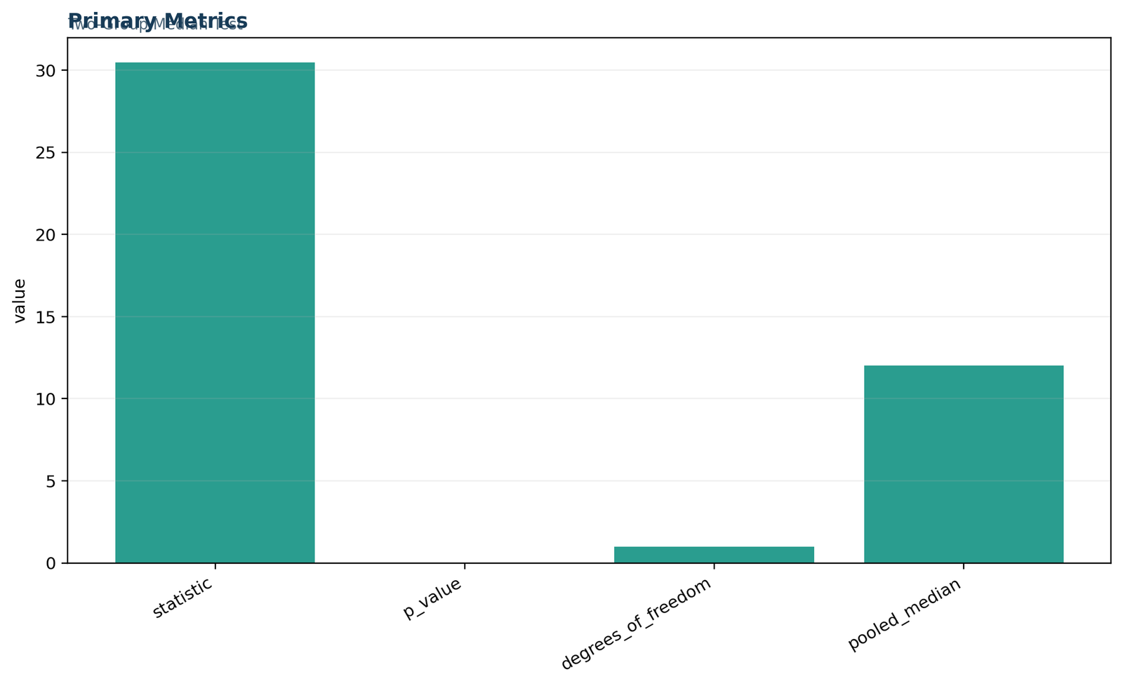
In this worked Median Test example, the outcome variable is G3 and the grouping variable is school, coded as GP and MS. The Median Test first computes one pooled median from all 649 observations. That pooled median is 12. Each score is then classified as above the pooled median or at or below the pooled median. The observed 2 × 2 table is GP: 213 above and 210 at/below, and MS: 63 above and 163 at/below. Applying the Pearson chi-square formula to that table yields χ² = 30.4516 with df = 1 and p = 3.422975281 × 10⁻⁸.
What does the Median Test measure?
The Median Test compares independent groups by examining how many observations fall above or at/below one pooled median.
The Median Test is a nonparametric method designed to answer a very direct question: do two or more independent groups appear to have the same median? Instead of working with means, pooled ranks, or raw score differences, the Median Test converts the data into a contingency table. First, one median is calculated from all observations combined. Then every value is classified relative to that pooled center. The resulting above-versus-below count pattern becomes the basis for a chi-square test.
Because of this structure, the Median Test is especially appealing when the research question is explicitly about medians or about central location defined in a robust, highly interpretable way. Analysts who do not want to rely on mean-based logic, and who prefer a simpler story than the one told by full rank-based procedures, often choose the Median Test for exactly that reason. It is conceptually clean, easy to teach, and easy to explain in public articles.
Why the Median Test is useful
The Median Test is useful because the median is a resistant measure of center. When outcomes are skewed, heavy-tailed, or influenced by outliers, the median often gives a more stable sense of the “typical” value than the mean. The Median Test takes that robust center seriously. Rather than testing a mean difference, it tests whether group membership is associated with being above or below the pooled median.
This means the Median Test belongs to the family of methods that connect nonparametric thinking with chi-square logic. In practice, that makes it easy to place beside guides on the Pearson Chi-Square Test, the G-Test, or the Likelihood Ratio Chi-Square. All of those procedures work with tables, but the Median Test uses the table as a way to compare centers across groups.
What the Median Test does not do
The Median Test is intentionally simple, and that simplicity creates both strengths and limitations. It does not use the full ordering information of all observations the way a Brunner Munzel Test or a Mann Whitney U Test does. It also does not estimate mean differences or probabilities directly the way a Relative Risk or Odds Ratio framework might in categorical-event settings.
So the best way to think about the Median Test is this: it answers a specific and public-friendly question very well, but it is not intended to replace every other nonparametric comparison method. It is best when the analyst truly wants a pooled-median interpretation.
The method also acts as a bridge between sign-style nonparametric reasoning and the larger family of chi-square methods. Readers who already understand contingency tables often grasp the Median Test quickly because the final inferential step is a familiar chi-square comparison. Meanwhile, readers who care most about robust center are attracted to the fact that the entire method revolves around the median.
In public-facing statistics writing, that bridge is valuable. Many readers can see that one group seems higher than another from a box plot or a table of medians, but they want to know whether the difference is statistically meaningful. The Median Test gives them a direct answer without requiring a normality-based model or a complex rank-sum explanation.
Another strength of the Median Test is that it promotes disciplined interpretation. Because the procedure explicitly classifies observations relative to a pooled center, it keeps the reader focused on the idea of central tendency rather than letting the discussion drift toward exaggerated claims about every part of the distribution. That narrow focus is often a benefit, especially in public educational content.
When should you use the Median Test?
Use the Median Test when the design contains independent groups and the research question is about differences in median location.
A common search phrase is when to use the Median Test or when to use Mood’s median test. The practical answer is simple: choose the Median Test when you want a nonparametric test of central tendency based specifically on the median, and when your groups are independent. It can be especially attractive when the raw variable is skewed, when the mean would be sensitive to extreme values, or when the audience will understand the median more naturally than a rank-based probability or a mean-based effect.
Independent groups
The groups must be separate, such as GP versus MS schools or treatment versus control.
Rankable or numeric outcome
The outcome must be measurable on at least an ordinal scale so that the notion of being above or below the pooled median is meaningful.
Median-focused question
The main inferential target should be a difference in medians or central location, not a mean difference.
Robust preference
Use the Median Test when a resistant center is preferable because of skewness, outliers, or non-normality.
Simple public explanation
The Median Test is excellent when the result needs to be explained clearly to non-specialists.
Situations that fit the Median Test well
Situations where another method may fit better
Another reason the Median Test remains popular is its communicative clarity. A public reader does not need to master all of nonparametric statistics to understand the simple idea that one group has more values above the pooled median than would be expected under the null hypothesis. This makes the Median Test especially attractive in educational, healthcare, policy, and social-science contexts.
It is also useful in applied datasets that contain unequal group sizes, ties, and irregular score patterns. The current example has 423 GP students and 226 MS students. Even with those unequal sample sizes, the Median Test remains straightforward because it uses observed counts and expected counts computed from marginal totals.
Finally, the Median Test is often helpful as a teaching companion to other methods. A reader may first understand the pooled-median table and then move on to more detailed procedures such as the Ansari-Bradley Test for scale differences or the Sign Test for related nonparametric logic. In that sense, the Median Test is not only an endpoint; it is also a conceptual stepping stone.
Median Test assumptions
The Median Test is flexible, but like all statistical procedures, it still depends on a few important design assumptions.
The Median Test assumptions are lighter than many parametric assumptions, but they matter. The groups should be independent, the outcome should support a meaningful notion of central tendency, the pooled median should be computed from the full sample before classification, and the expected counts should be large enough for the chi-square approximation to be appropriate. The Median Test does not require a normal distribution, which is one reason it is regularly introduced in nonparametric modules.
Independent samples
The GP and MS school groups are nonoverlapping. Each student belongs to one school category only, satisfying the independence requirement for the Median Test.
Meaningful center
The response variable G3 is numeric and supports a meaningful median. This makes the pooled-median classification interpretable.
One pooled median
The pooled median is computed from all 649 observations together before any group-specific counting occurs. This is a defining feature of the Median Test.
Tie handling rule
Scores equal to the pooled median are assigned to the at or below category. This tie rule is explicitly documented in the workbook and must be applied consistently.
Expected count adequacy
The expected counts are 179.8891, 243.1109, 96.1109, and 129.8891, all comfortably above common minimum thresholds for chi-square use.
Correct inferential target
The Median Test is aimed at comparing medians through a 2 × 2 table. If the substantive goal is different, another method may be better aligned.
Good analysts therefore check assumptions before jumping to the p-value. They confirm that the groups are truly independent, that the response variable supports a meaningful median, that the pooled center was defined once for all observations, and that the expected counts justify the chi-square approximation. Those checks make the Median Test much easier to defend and much easier to explain responsibly.
The present worked example satisfies those assumptions well. The design is independent, the outcome variable is numeric, the tie rule is explicit, and all expected frequencies are comfortably large. That makes the Median Test a natural and defensible tool for this problem.
It is worth emphasizing that “natural” does not mean automatic. A careful analyst always verifies that the median is really the center of interest. In the current setting, the median is a sensible focus because the variable is a final-grade score with many repeated values, and the public question centers on whether the typical grade level differs by school type.
Null and alternative hypotheses
The Median Test expresses the median-comparison question through a pooled-median contingency framework.
Null hypothesis
H0: the groups come from populations with the same median. Equivalently, once the pooled median is fixed, group membership is not associated with whether an observation falls above the pooled median or at/below it.
In this worked example, the null says that GP and MS students should show the same above-versus-below-median pattern after the pooled median of 12 is defined.
Alternative hypothesis
H1: the groups do not share the same median. Equivalently, group membership is associated with the probability of being above the pooled median.
For the current example, that means GP and MS students would show different above-versus-below-median patterns if the alternative is true.
G3 final grade
school = GP or MS
two independent samples
This hypothesis structure is one reason the Median Test is so teachable. The null says that group membership should not matter once values are classified relative to the pooled median. The alternative says that it does matter. The later chi-square calculation is therefore just a formal way of measuring how far the observed classification table departs from the pattern expected under the null.
For teaching purposes, the hypothesis section is often where the Median Test becomes most intuitive. The null says neither school has a systematic advantage in placing students above the pooled median. The alternative says one school does have that advantage. Once that is understood, the observed and expected counts become much easier to read.
This hypothesis framing also keeps the Median Test tied to the idea of central location instead of drifting into unrelated claims. The procedure does not prove that every GP student scores higher than every MS student, nor does it claim that the groups differ equally at every point in the distribution. It answers the narrower, and often very important, question of whether the group medians are the same.
Median Test formula and calculation steps
The Median Test uses a Pearson chi-square statistic computed from the contingency table formed by the pooled median classification.
This is the core Median Test statistic. After the pooled median is computed, each group contributes observed counts in the above median and at or below median categories. The difference between those observed counts and their expected counts is summarized through the Pearson chi-square formula.
The expected count for each cell equals the product of the corresponding row total and column total divided by the total sample size. In the current Median Test, that rule produces expected counts of 179.8891 and 243.1109 for the GP row, and 96.1109 and 129.8891 for the MS row.
The pooled median is not the average of the group medians. Instead, it is one single median computed from the entire sample combined. In this worked example, the pooled median is 12. Scores equal to 12 are placed in the at or below category according to the workbook’s tie rule.
The calculation logic of the Median Test is compact but meaningful. First, all observations from GP and MS are combined to produce one pooled median. Second, each observation is converted into a binary classification relative to that pooled center. Third, the observed counts in the resulting 2 × 2 table are compared with the counts expected under the null hypothesis. Fourth, those deviations are aggregated through the chi-square formula. Finally, the statistic is compared with the chi-square distribution with 1 degree of freedom to obtain the p-value.
Exact calculation components
What the numbers mean
The GP group contributes more above-median observations than expected under the null and fewer at/below observations than expected. The MS group shows the reverse pattern. Those departures are large enough to produce χ² = 30.4516 and a very small p-value. In other words, the observed above-versus-below-median pattern is far too imbalanced to be explained by ordinary sampling variation if the group medians were truly the same.
A simple derived effect-size view also helps: phi = √(χ²/N) = 0.2166. This is not the official statistic of the Median Test itself, but it gives a compact sense of the strength of association in the resulting 2 × 2 table.
The mathematical benefit of this presentation is that the Median Test becomes auditable. A reader can trace the analysis from raw data to pooled median, from pooled median to contingency table, and from the table to the chi-square statistic and p-value. That transparency is one reason the Median Test remains useful in public educational statistics.
It also makes the result easy to defend. If a reader asks why the p-value is so small, the answer is visible in the strong departures between observed and expected counts. If the reader asks why GP is interpreted as higher, the answer comes from the fact that GP contributes many more above-median observations than the null would predict, while MS contributes many fewer.
Variables used in the worked example
A clear data dictionary makes the Median Test easier to read, verify, and explain.
| Variable | Role | Description |
|---|---|---|
| G3 | Outcome variable | Final-grade score used to compute the pooled median and the above/below classification for the Median Test. |
| school | Grouping variable | Independent grouping variable with categories GP and MS. |
| GP | Group 1 | 423 students in the GP school category. |
| MS | Group 2 | 226 students in the MS school category. |
| Above median | Derived classification | Indicator equal to 1 when G3 is strictly greater than the pooled median of 12. |
| At or below | Derived classification | Indicator equal to 1 when G3 is equal to or less than the pooled median of 12. |
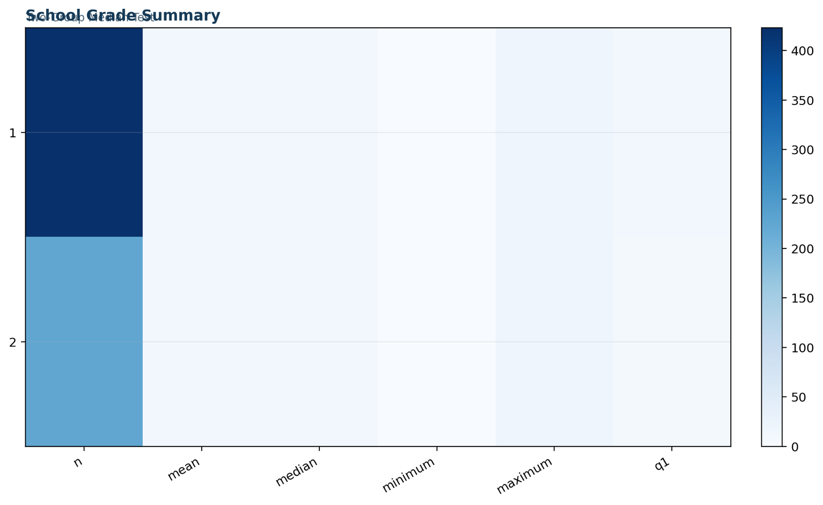
These descriptive statistics already suggest the eventual Median Test result. The GP group has a median of 13, while the MS group has a median of 11. The GP group also has a higher mean and a slightly higher upper quartile. The pooled-median analysis formalizes that descriptive difference into a statistical test.
Public readers often understand a method better when descriptive and inferential layers are presented together. That is why this guide keeps the data dictionary, summary statistics, pooled-median explanation, and formal Median Test result close to each other instead of scattering them across unrelated sections.
The variable section also prevents a common reporting problem: software output can be numerically correct but semantically vague. Naming G3 and school explicitly ensures that the Median Test is not reduced to anonymous symbols. This makes the final article more readable for both technical and nontechnical audiences.
Worked example: final grades by school type
The worked example shows exactly how the Median Test turns raw data into a pooled-median contingency analysis.
The worked Median Test example compares final grades between students in GP schools and students in MS schools. The first step is to compute the pooled median across all observations. That pooled median equals 12. Every final-grade value is then classified relative to that threshold. Scores of 13 or higher count as above median, while scores of 12 or lower count as at or below median under the workbook’s tie rule.
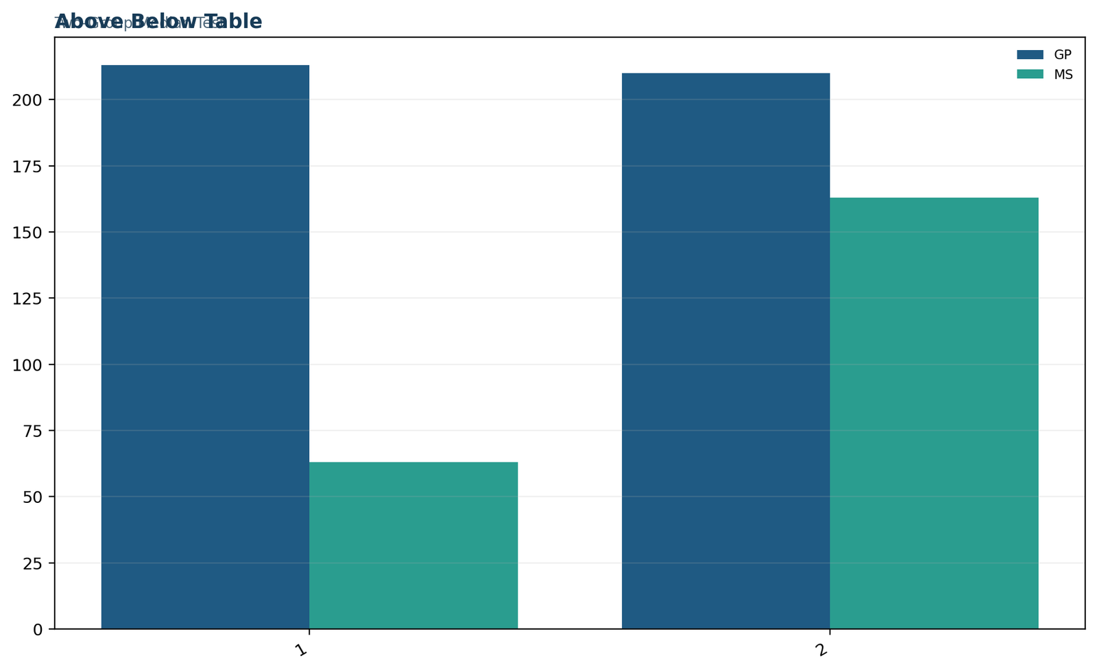
Once the classification is complete, the observed table is straightforward. In the GP group, 213 observations are above the pooled median and 210 are at or below it. In the MS group, only 63 observations are above the pooled median, while 163 are at or below it. Those observed counts already tell a compelling story: GP students are much more likely to appear above the pooled median than MS students.
How the count story reads in plain language
The Median Test does not say that every GP student outperforms every MS student. Instead, it says that once one common median is defined, the GP group contributes many more above-median observations than expected under equal medians, while the MS group contributes fewer. That is the key evidence for rejecting the null hypothesis.
This distinction matters because public readers sometimes overread statistical findings. The Median Test detects a difference in central location through the classification pattern. It does not imply perfect separation or deterministic dominance.
Observed two-group result
The chi-square comparison of the pooled-median table indicates a statistically significant difference.
At the 0.05 significance level, the null hypothesis of equal medians is rejected. The GP school group tends to have a higher final-grade center than the MS group.
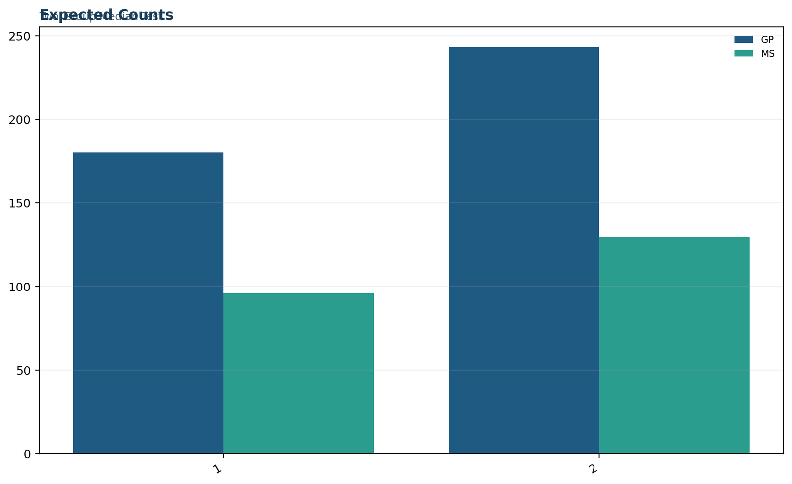
The expected-count table makes the interpretation even clearer. Under the null hypothesis, GP would be expected to contribute only about 179.89 above-median scores, yet it contributes 213. Under the same null, MS would be expected to contribute about 96.11 above-median scores, yet it contributes only 63. The imbalance is large, consistent, and directionally coherent.
The worked example therefore shows how a highly technical question can still be expressed in a readable public language. The statistic and p-value satisfy formal reporting standards, the observed-versus-expected table shows exactly where the difference comes from, and the descriptive medians of 13 versus 11 give the public a concrete sense of what the result means.
This is one of the strongest teaching features of the Median Test. A reader can see the path from raw values to pooled center to classified table to final inference without having to rely on hidden calculations or black-box software output.
Exact Median Test results table
The main numerical outputs are easiest to understand when gathered in one structured summary table.
| Metric | Value | Interpretation |
|---|---|---|
| Group 1 | GP | School group with the higher observed number of above-median scores. |
| Group 2 | MS | School group with fewer above-median scores than expected. |
| Sample sizes | 423 and 226 | Unequal group sizes handled through the contingency-table framework of the Median Test. |
| Pooled median | 12 | Common reference point used for classification. |
| Observed GP counts | 213 above, 210 at/below | GP contributes nearly half above the pooled median. |
| Observed MS counts | 63 above, 163 at/below | MS contributes many fewer above-median observations. |
| Expected GP counts | 179.8891 above, 243.1109 at/below | Expected under equal medians. |
| Expected MS counts | 96.1109 above, 129.8891 at/below | Expected under equal medians. |
| Chi-square statistic | 30.4516190523 | Strong deviation from the null pattern. |
| Degrees of freedom | 1 | 2 × 2 table with one degree of freedom. |
| P-value | 3.422975281 × 10⁻⁸ | Very strong evidence against equal medians. |
| Derived phi coefficient | 0.2166 | Compact effect-size view of the association in the table. |
What the result table means in plain language
The Median Test table shows that the GP group contributes more observations above the pooled median than expected, while the MS group contributes fewer. Because this mismatch between observed and expected counts is so large, the chi-square statistic is large and the p-value is extremely small. The evidence therefore supports the conclusion that the two groups do not share the same median final grade.
One reason this table is useful is that it keeps the entire story together: the pooled center, the classification counts, the expected counts, the chi-square result, and the interpretation. When those pieces are presented together, the Median Test becomes much easier to explain both technically and publicly.
A result table like this also reduces ambiguity about what exactly was tested. The reader can see that the procedure is not a mean-based t test, not a full-rank comparison, and not a probability-ratio analysis. It is specifically a Median Test grounded in the observed-versus-expected pattern above and at/below the pooled median.
How to interpret the Median Test
Interpretation should combine significance, direction, and substantive meaning.
Many readers search how to interpret the Median Test or what does a significant Median Test mean. A complete interpretation should report the chi-square statistic, the p-value, the pooled median, the observed count pattern, and a plain-language statement about which group tends to have the higher center.
Statistical decision
Because the p-value is 3.422975281 × 10⁻⁸, the null hypothesis of equal medians is rejected. The two groups do not appear to share the same median final grade.
Direction of the difference
The GP group contributes more above-median observations than expected, while the MS group contributes fewer. That direction is consistent with the descriptive medians of 13 for GP and 11 for MS.
Practical meaning
The result suggests that the typical final-grade location is higher in the GP school group than in the MS school group. The finding is statistically strong and easy to explain publicly.
The most useful public interpretation is therefore: a Median Test showed that final-grade medians differ significantly by school type, with the GP group tending to occupy the higher side of the pooled-median split more often than the MS group. That is a concise sentence, but it faithfully reflects the observed counts, the chi-square statistic, and the descriptive medians.
Good interpretation also avoids overclaiming. The Median Test does not by itself prove why the two groups differ. It does not establish causality, nor does it claim that the two school groups differ in every possible distributional feature. What it does establish is that the median-centered classification pattern is strongly associated with school type.
This balance between evidence and restraint is especially important in public statistics writing. The evidence of a difference is clear, but the explanation of the cause would require broader design information or additional modeling. Responsible reporting says both things at once.
It is equally important not to undersell the result. The p-value is extraordinarily small, the observed-versus-expected discrepancies are large, and the descriptive medians point in the same direction. So the evidence that the GP and MS school groups differ in median location is not marginal—it is strong.
Median Test in Python: chart-by-chart interpretation
The Python figures explain the pooled-median logic visually from the main metric to the final summary.
Searchers often want a Median Test in Python example that does more than print a single p-value. The Python chart set below explains the same result visually while preserving the exact boxed-chart format used in the permanent site design.
Python is especially useful for teaching the Median Test because each stage of the procedure can be scripted transparently. The pooled median can be computed directly, each observation can be classified in code, expected counts can be verified, and the chi-square statistic can be reproduced step by step. That transparency makes the figure set below especially valuable for educational readers.
Python chart 1: primary metrics
This opening figure acts as the dashboard of the entire Median Test result. It highlights the main numerical outputs—χ² = 30.4516, p = 3.422975281 × 10⁻⁸, pooled median = 12, and the sample sizes for GP and MS. The chart tells the central story immediately: the two groups differ strongly on the median-based classification.
Python chart 2: above/below table
This chart displays the observed 2 × 2 table that drives the Median Test. It makes the central imbalance visually obvious. GP contributes many more above-median scores than MS, and MS contributes many more at/below-median scores. For public readers, this is often the most intuitive visual in the entire analysis.
Python chart 3: expected counts
The expected-count chart adds inferential meaning to the observed table. Under the null hypothesis, GP should contribute only about 179.89 above-median observations, but it actually contributes 213. Under the same null, MS should contribute about 96.11 above-median observations, but it actually contributes only 63. These gaps are exactly what produce the large chi-square statistic.
Python chart 4: school grade summary
This descriptive figure shows why the Median Test detects a difference. GP has a higher median, a higher mean, and a slightly stronger upper-half profile than MS. The descriptive pattern therefore aligns neatly with the chi-square evidence from the pooled-median table.
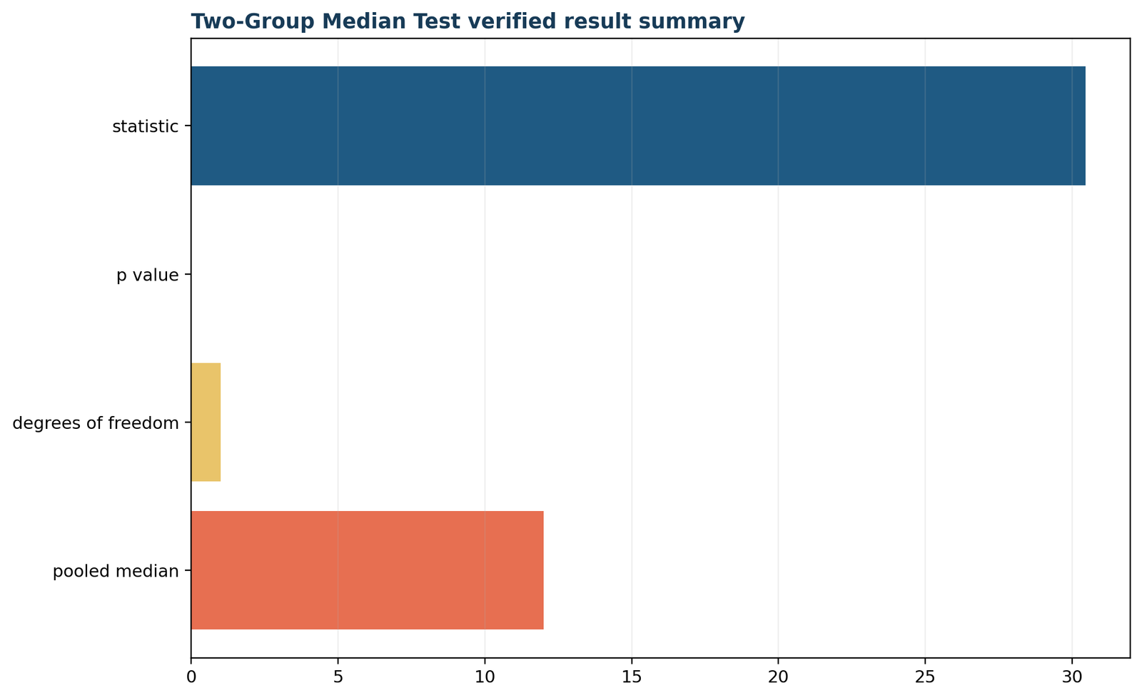
Python chart 5: verified result summary
This final Python chart condenses the full Median Test story into a public-ready conclusion: the GP and MS groups do not share the same median final grade, and the GP group shows a systematically stronger presence above the pooled median.
For learners, the Python visuals also help separate descriptive evidence from inferential evidence. The descriptive figure shows how the groups look, the observed table shows what the classification counts are, the expected-count chart explains why the chi-square statistic becomes large, and the summary figure tells the final story in one glance. Taken together, the five Python charts provide a compact learning sequence for the Median Test.
Median Test in R: chart-by-chart interpretation
The R figures reinforce the same substantive message and strengthen reproducibility across software platforms.
The Median Test in R is commonly used in teaching and applied analysis. The R chart set confirms that the result does not depend on one software environment alone. When Python and R converge on the same pooled median, contingency pattern, chi-square statistic, and p-value, confidence in the analysis naturally increases.
R is also a strong environment for the Median Test because it combines data wrangling, tables, graphics, and report writing in one place. The boxed figures below therefore do more than repeat the Python visuals—they reinforce the analytical reliability of the same conclusion.
R chart 1: primary metrics
The first R chart confirms the same main outputs as the Python analysis. The Median Test remains highly significant, the pooled median remains 12, and the overall inference is unchanged.
R chart 2: above/below table
This chart reiterates the exact observed classification table. The visual emphasis makes it easy to see that GP contributes a much larger above-median count than MS, which is precisely what the Median Test detects.
R chart 3: expected counts
The expected-count figure helps readers connect the intuitive table story with the formal chi-square calculation. The discrepancies between observed and expected counts are large and consistent, which explains the strength of the p-value.
R chart 4: school grade summary
This descriptive chart reconnects the Median Test result to the original data scale. The GP group has a higher descriptive center than the MS group, so the inferential conclusion does not appear in isolation; it is grounded in the raw score summaries.
R chart 5: verified result summary
The last R figure compresses the full Median Test analysis into a concise public conclusion: school type is associated with the above-versus-below pooled-median pattern, and the GP group tends to show the higher median location.
That reproducibility matters in public-facing statistics. When the same Median Test conclusion appears in both Python and R, readers gain confidence that the result is anchored in the data rather than in one interface or one package default. Cross-software agreement is therefore part of the explanation, not merely an extra technical detail.
Median Test in SPSS
SPSS users reach the same inferential conclusion, even though the output interface looks different.
SPSS interpretation points
In SPSS, the Median Test is still read through the same core ingredients: the pooled median, the above/below classification, the observed-versus-expected count differences, the chi-square statistic, and the significance level. A good SPSS interpretation should also mention which group contributes more above-median observations, rather than stopping at significance alone.
Publicly, it helps to explain that the SPSS result is not merely a generic chi-square table. It is specifically the chi-square table generated by a pooled-median classification. That keeps the interpretation aligned with what the Median Test actually measures.
SPSS conclusion for this example
The SPSS output agrees with the workbook and with the Python/R analyses: the GP and MS groups differ significantly in their median-centered classification pattern, and the GP group tends to occupy the higher side of the pooled median more often. The interface changes, but the substantive meaning does not.
This cross-platform agreement is good for public trust. It shows that the result is not an artifact of one coding environment but a stable conclusion supported across the main analysis tools.
Median Test in Excel
The workbook makes every classification and expected-count step visible, which is extremely useful for teaching and auditability.
Searchers often ask how to do a Median Test in Excel or how to calculate Mood’s median test in Excel. The workbook used here answers that question transparently. Excel is especially useful because it exposes the raw data, the pooled-median classification, the contingency counts, the expected counts, the chi-square calculation, and the reporting cross-checks in separate, auditable sheets.
| Workbook sheet | Purpose in the Median Test workflow |
|---|---|
| Guide | Documents the design, null hypothesis, formula, and workbook scope. |
| Data_Input | Stores the unchanged analysis variables G3 and school. |
| Working | Shows the pooled median and the above-versus-at/below classification for every observation. |
| Calculations | Displays observed counts, expected counts, chi-square, degrees of freedom, p-value, and N. |
| Diagnostics | Lists the pooled-center rule, tie rule, and expected-count logic. |
| Reporting | Cross-checks workbook outputs against independently verified reference values. |
This transparency matters for educational SEO content because many readers want to understand not only the answer but also the route to the answer. A workbook that shows every intermediate step makes the Median Test easier to learn, easier to verify, and easier to trust.
Excel also slows the analysis down in a productive way. Instead of clicking one menu option and accepting an opaque output, the learner can inspect each intermediate component. That makes the Median Test feel less like a mysterious software routine and more like a logical argument built from a pooled center and a 2 × 2 table.
How to report Median Test results
Good reporting tells readers what was compared, how it was compared, and what the comparison means.
Many public posts stop after printing a p-value. A better Median Test report names the groups, states the pooled median, gives the chi-square statistic and p-value, mentions the observed direction of the classification pattern, and offers a readable explanation of what that pattern means for the medians. This richer approach turns software output into meaningful interpretation.
APA-style example
A Median Test was conducted to compare final grades between GP and MS school groups. Using a pooled median of 12, scores were classified as above the pooled median or at/below it. The resulting 2 × 2 table showed a statistically significant association between school type and median classification, χ2(1, N = 649) = 30.45, p < .001. The GP group contributed more above-median scores than expected under the null hypothesis, indicating a higher median-centered performance pattern than the MS group.
What to include
- Name the Median Test explicitly.
- Report the pooled median.
- Report χ2, df, and the p-value.
- State the observed count direction.
- Connect the result back to the median comparison in plain language.
What to avoid
- Do not report only that the result is significant without the pooled-median context.
- Do not describe the method as if it were a mean-comparison test.
- Do not ignore the tie rule if scores equal the pooled median are present.
- Do not overstate the result as causal when the analysis is only comparative.
The best public explanation therefore combines the formal and the intuitive: the Median Test was significant, the GP group contributed more above-median scores than expected, and the descriptive medians of 13 versus 11 show the same direction on the original scale. That is technically sound and still readable for general audiences.
Reporting quality is often the most overlooked part of applied statistics. A result can be computed perfectly and still communicated badly. By contrast, a well-written Median Test report makes the method, the result, and the substantive meaning all visible at once. That is the reporting standard this guide aims to model.
Median Test versus related methods
Different nonparametric and categorical methods answer different questions, so the method should match the inferential target.
| Method | Main question | How it differs from the Median Test |
|---|---|---|
| Median Test | Do independent groups differ in median location? | Uses one pooled median and a chi-square test on above/below counts. |
| Brunner Munzel Test | Do two independent groups differ in stochastic dominance? | Uses richer ranking information rather than collapsing values into two categories. |
| Ansari-Bradley Test | Do two groups differ in scale? | Targets variability or scale, not median location. |
| Conover Test / Dunn’s Test | Which groups differ after a multi-group omnibus result? | Post hoc pairwise procedures rather than pooled-median omnibus tests. |
| Pearson Chi-Square Test | Is there association in a contingency table? | The Median Test uses Pearson chi-square, but specifically on a table created from a pooled-median classification. |
| Fisher’s Exact Test | Is there exact association in a small contingency table? | Targets categorical association directly; not designed as a median-comparison method. |
| Fisher-Freeman-Halton Test | Exact association in larger tables | General categorical exact test rather than a median-focused procedure. |
| McNemar’s Test / McNemar-Bowker Test | Do paired categorical responses change? | For paired designs, whereas the Median Test is for independent groups. |
| Mantel-Haenszel Test | Is there a stratified association? | Combines information across strata rather than classifying one outcome relative to a pooled median. |
| Z Test for Proportions | Do two proportions differ? | Works on binary outcomes directly, not on a binary table created from a continuous outcome’s pooled median. |
This comparison table shows that the Median Test has a clear place in the broader methodological landscape. It is neither a universal replacement for all nonparametric methods nor a redundant version of every chi-square test. It is a specific tool for a specific question: whether the median-centered classification pattern differs across independent groups.
Readers also often search for conceptual neighbors such as Weighted Kappa, Fleiss Kappa, or a general Kappa Statistic. Those are agreement measures, not median-comparison tools. Bringing them into the comparison reminds readers that a statistical method should always be chosen because it matches the research question, not merely because it is familiar.
That is the central methodological lesson. Good analysis begins by asking what kind of difference matters most—median difference, scale difference, paired change, distributional dominance, categorical association, or agreement. The Median Test is excellent when the median-centered comparison is the right language for the real question.
Downloads
These links provide the supporting materials used in the worked example.
Python reportDetailed Python output and interpretation for the Median Test.Open report
R reportR output for the same pooled-median comparison.Open report
SPSS outputSPSS companion output for the worked example.Open report
Excel workbookAuditable workbook with pooled-median classification, expected counts, and reporting checks.Open workbook
Frequently asked questions about the Median Test
Short answers to common questions about the method, its assumptions, and its interpretation.
What is the Median Test?
The Median Test is a nonparametric method that compares independent groups by classifying observations relative to one pooled median and then applying a chi-square test.
Is the Median Test the same as Mood’s median test?
Yes. In many textbooks and software discussions, the Median Test is also called Mood’s median test.
What was the pooled median in this example?
The pooled median used in this worked example was 12.
What were the school groups in the worked example?
The two groups were GP and MS schools.
What was the test statistic?
The observed Median Test statistic was χ² = 30.4516190523.
What was the p-value?
The p-value was 3.422975281 × 10⁻⁸, which is far below 0.05.
Was the Median Test significant?
Yes. The result was highly statistically significant, so the null hypothesis of equal medians was rejected.
Which group tended to have the higher median?
The GP group tended to have the higher median-centered pattern, supported by both the descriptive median of 13 and the above-median count structure.
Does the Median Test require normality?
No. The Median Test is nonparametric and does not require a normal distribution.
How are ties treated in the Median Test?
In this workbook, scores equal to the pooled median are classified as at or below. That tie rule must be stated clearly when reporting the Median Test.
Why are expected counts important?
The expected counts show what the table should look like under equal medians. The chi-square statistic measures how far the observed table departs from those expectations.
Is the Median Test always better than the Mann Whitney U test?
No. The Median Test is simpler and more directly centered on the median, but the Mann Whitney U test uses more ordering information and can be more powerful in many settings.
Can unequal group sizes be used in the Median Test?
Yes. This example uses 423 GP observations and 226 MS observations, and the method handles that through expected counts based on the marginal totals.
Can the Median Test be done in Excel?
Yes. The workbook linked in this guide shows every step, from pooled median calculation to the final reporting table.
Can the Median Test be done in Python and R?
Yes. This guide includes matched Python and R chart explanations along with downloadable reports.
Why is the Median Test considered robust?
The Median Test is considered robust because it is centered on the median, which is less sensitive to extreme values than the mean.
What is the main conclusion of this worked example?
The Median Test shows that the GP and MS school groups differ significantly in their median final-grade pattern, with GP tending to occupy the higher side of the pooled median more often.