
.abx-article{–ink:#102238;–muted:#52657a;–line:#dce5ed;–paper:#fff;–soft:#f4f8fb;–navy:#092a45;–teal:#0d7774;–cyan:#dff7f6;–amber:#f4a340;–amber-soft:#fff4df;–red:#a83232;–red-soft:#fff0f0;–green:#176b47;–green-soft:#e9f8f0;–violet:#6654b8;–violet-soft:#f0edff;–shadow:0 16px 45px rgba(18,44,67,.10);font-family:Inter,ui-sans-serif,system-ui,-apple-system,BlinkMacSystemFont,”Segoe UI”,Arial,sans-serif;color:var(–ink);line-height:1.72;display:block;width:100%!important;max-width:100%!important;margin:0 auto!important;background:var(–paper);font-size:17px;overflow-x:clip}
.abx-article *{box-sizing:border-box}.abx-article a{color:#075f72;text-decoration-thickness:1px;text-underline-offset:3px}.abx-article a:hover{color:#043f4c}.abx-shell{width:100%;max-width:1480px;margin:0 auto;padding:clamp(18px,2.8vw,42px)}.abx-hero{position:relative;overflow:hidden;border-radius:28px;background:linear-gradient(132deg,#07263f 0%,#0b4b61 55%,#0a7770 100%);color:#fff;padding:clamp(28px,6vw,68px);box-shadow:var(–shadow)}.abx-hero:before{content:””;position:absolute;right:-90px;top:-120px;width:360px;height:360px;border-radius:50%;background:rgba(255,255,255,.07)}.abx-hero:after{content:””;position:absolute;left:-110px;bottom:-180px;width:390px;height:390px;border-radius:50%;background:rgba(244,163,64,.10)}.abx-hero>*{position:relative;z-index:1}.abx-kicker{display:inline-flex;align-items:center;gap:9px;padding:7px 12px;border:1px solid rgba(255,255,255,.25);border-radius:999px;background:rgba(255,255,255,.09);font-size:.78rem;font-weight:800;letter-spacing:.08em;text-transform:uppercase}.abx-kicker i{width:9px;height:9px;border-radius:50%;background:#ffbd62;box-shadow:0 0 0 5px rgba(255,189,98,.16)}.abx-hero h1{font-size:clamp(2.15rem,5.2vw,4.65rem);line-height:1.04;letter-spacing:-.045em;margin:22px 0 18px;max-width:1000px;color:#fff}.abx-hero .abx-lead{font-size:clamp(1.05rem,2vw,1.34rem);max-width:900px;color:#e9f7fb;margin:0}.abx-badges{display:flex;flex-wrap:wrap;gap:10px;margin-top:25px}.abx-badge{padding:8px 12px;border-radius:999px;background:rgba(255,255,255,.11);border:1px solid rgba(255,255,255,.19);font-size:.84rem;font-weight:750}.abx-hero-result{margin-top:28px;display:grid;grid-template-columns:repeat(4,minmax(0,1fr));gap:12px}.abx-hero-metric{background:rgba(255,255,255,.10);border:1px solid rgba(255,255,255,.16);border-radius:16px;padding:14px}.abx-hero-metric span{display:block;color:#cdeaf0;font-size:.78rem;text-transform:uppercase;letter-spacing:.05em;font-weight:800}.abx-hero-metric strong{display:block;margin-top:4px;font-size:1.28rem;color:#fff}.abx-ad{display:flex;align-items:center;justify-content:center;min-height:96px;margin:26px 0;border:1px dashed #b8c6d1;border-radius:18px;background:#f8fafc;color:#718096;font-size:.78rem;letter-spacing:.14em;text-transform:uppercase}.abx-quick{display:grid;grid-template-columns:1.35fr .65fr;gap:20px;margin:28px 0}.abx-card{min-width:0;max-width:100%;border:1px solid var(–line);border-radius:22px;background:#fff;box-shadow:0 10px 30px rgba(21,48,70,.06);padding:clamp(19px,3vw,30px)}.abx-card h2,.abx-card h3{margin-top:0}.abx-answer{background:linear-gradient(145deg,#f2fbfa,#fff);border-color:#bfe5e2}.abx-answer .abx-verdict{display:inline-flex;align-items:center;gap:9px;padding:8px 12px;border-radius:999px;background:var(–green-soft);color:var(–green);font-weight:850;font-size:.84rem}.abx-answer .abx-verdict:before{content:”✓”;display:grid;place-items:center;width:22px;height:22px;border-radius:50%;background:var(–green);color:#fff}.abx-answer h2{font-size:clamp(1.55rem,3vw,2.25rem);line-height:1.15;margin:15px 0 10px}.abx-mini-table{display:grid;gap:10px}.abx-mini-row{display:flex;justify-content:space-between;gap:20px;padding:11px 0;border-bottom:1px solid var(–line)}.abx-mini-row:last-child{border-bottom:0}.abx-mini-row span{color:var(–muted)}.abx-mini-row strong{text-align:right}.abx-toc{margin:26px 0;border-radius:22px;background:var(–navy);color:#fff;padding:24px}.abx-toc h2{color:#fff;margin:0 0 14px;font-size:1.2rem}.abx-toc-grid{display:grid;grid-template-columns:repeat(3,minmax(0,1fr));gap:8px 20px}.abx-toc a{color:#d9f6f5;text-decoration:none;padding:7px 0;display:block;border-bottom:1px solid rgba(255,255,255,.12)}.abx-toc a:hover{color:#fff}.abx-section{scroll-margin-top:24px;margin:54px 0}.abx-section-head{display:grid;grid-template-columns:auto 1fr;align-items:start;gap:14px;margin-bottom:20px}.abx-num{width:42px;height:42px;border-radius:13px;background:var(–navy);color:#fff;display:grid;place-items:center;font-weight:900}.abx-section-head h2{margin:0;font-size:clamp(1.65rem,3.4vw,2.65rem);line-height:1.15;letter-spacing:-.025em}.abx-section-head p{grid-column:2;margin:5px 0 0;color:var(–muted);max-width:920px}.abx-grid-2{display:grid;grid-template-columns:repeat(2,minmax(0,1fr));gap:20px}.abx-grid-2>*,.abx-grid-3>*,.abx-grid-4>*,.abx-chart-grid>*,.abx-downloads>*,.abx-related>*,.abx-quick>*{min-width:0}.abx-grid-3{display:grid;grid-template-columns:repeat(3,minmax(0,1fr));gap:18px}.abx-grid-4{display:grid;grid-template-columns:repeat(4,minmax(0,1fr));gap:14px}.abx-callout{border-radius:18px;padding:18px 20px;border-left:5px solid var(–teal);background:var(–cyan);margin:20px 0}.abx-callout strong{color:#084f4c}.abx-warning{border-left-color:var(–red);background:var(–red-soft)}.abx-warning strong{color:var(–red)}.abx-note{border-left-color:var(–amber);background:var(–amber-soft)}.abx-note strong{color:#875311}.abx-formula{border:1px solid #cbd8e3;background:linear-gradient(180deg,#fff,#f7fafc);border-radius:20px;padding:22px;margin:18px 0;text-align:center;overflow:visible}.abx-formula .eq{font-family:”Cambria Math”,”Times New Roman”,serif;font-size:clamp(1.08rem,2.2vw,1.5rem);white-space:normal;overflow-wrap:anywhere;word-break:normal;line-height:1.55}.abx-formula p{margin:8px auto 0;color:var(–muted);max-width:850px;text-align:left;font-size:.94rem}.abx-pill-list{display:flex;flex-wrap:wrap;gap:10px;margin:15px 0}.abx-pill{background:var(–soft);border:1px solid var(–line);border-radius:999px;padding:8px 12px;font-weight:750;font-size:.88rem}.abx-flow{display:grid;grid-template-columns:repeat(5,minmax(0,1fr));gap:10px;counter-reset:flow}.abx-step{position:relative;padding:18px 14px 16px;border:1px solid var(–line);border-radius:18px;background:#fff;min-height:148px}.abx-step:before{counter-increment:flow;content:counter(flow);display:grid;place-items:center;width:30px;height:30px;border-radius:10px;background:var(–teal);color:#fff;font-weight:900;margin-bottom:10px}.abx-step h3{font-size:1rem;margin:0 0 6px}.abx-step p{font-size:.9rem;color:var(–muted);margin:0}.abx-table-wrap{min-width:0;max-width:100%;overflow-x:auto;border:1px solid var(–line);border-radius:18px;background:#fff}.abx-table{width:100%;border-collapse:collapse;min-width:720px}.abx-table.abx-compact{min-width:0}.abx-table th{background:var(–navy);color:#fff;text-align:left;padding:13px 14px;font-size:.85rem;letter-spacing:.02em}.abx-table td{padding:13px 14px;border-bottom:1px solid var(–line);vertical-align:top}.abx-table tbody tr:nth-child(even){background:#f8fafc}.abx-table tbody tr:last-child td{border-bottom:0}.abx-stat-grid{display:grid;grid-template-columns:repeat(4,minmax(0,1fr));gap:12px;margin:16px 0}.abx-stat{border:1px solid var(–line);border-radius:16px;padding:16px;background:#fff}.abx-stat span{display:block;color:var(–muted);font-size:.78rem;font-weight:800;text-transform:uppercase;letter-spacing:.05em}.abx-stat strong{display:block;font-size:1.34rem;margin-top:4px}.abx-stat small{display:block;color:var(–muted);margin-top:4px}.abx-result-panel{border-radius:22px;background:linear-gradient(145deg,#082c47,#0b5966);color:#fff;padding:26px}.abx-result-panel h3{color:#fff;margin-top:0;font-size:1.45rem}.abx-result-panel p{color:#e5f6f7}.abx-result-panel .abx-result-big{font-size:clamp(2rem,5vw,3.7rem);line-height:1;font-weight:950;color:#fff;margin:10px 0}.abx-result-panel .abx-result-tag{display:inline-block;padding:8px 12px;border-radius:999px;background:rgba(255,255,255,.12);border:1px solid rgba(255,255,255,.18);font-weight:800}.abx-figure{min-width:0;max-width:100%;margin:0;border:1px solid var(–line);border-radius:22px;overflow:hidden;background:#fff;box-shadow:0 10px 30px rgba(21,48,70,.06)}.abx-figure img{display:block;width:100%;height:auto;background:#f3f6f8}.abx-figure figcaption{padding:18px 20px}.abx-figure h3{font-size:1.08rem;margin:0 0 6px}.abx-figure p{margin:0;color:var(–muted);font-size:.94rem}.abx-chart-grid{display:grid;grid-template-columns:repeat(2,minmax(0,1fr));gap:20px}.abx-chart-grid .abx-wide{grid-column:1/-1}.abx-code{min-width:0;max-width:100%;position:relative;background:#071d2d;color:#e6f2f7;border-radius:18px;overflow:auto;padding:20px;margin:16px 0;box-shadow:inset 0 0 0 1px rgba(255,255,255,.07)}.abx-code code{display:block;white-space:pre;min-width:max-content;font-family:”SFMono-Regular”,Consolas,”Liberation Mono”,monospace;font-size:.88rem;line-height:1.65}.abx-code-label{display:inline-block;margin-bottom:8px;color:#7ee7db;font-size:.76rem;font-weight:900;letter-spacing:.08em;text-transform:uppercase}.abx-downloads{display:grid;grid-template-columns:repeat(4,minmax(0,1fr));gap:14px}.abx-download{display:flex;flex-direction:column;min-height:190px;padding:20px;border-radius:20px;border:1px solid var(–line);background:#fff;text-decoration:none!important;color:var(–ink)!important;box-shadow:0 10px 30px rgba(21,48,70,.06);transition:.2s transform,.2s box-shadow}.abx-download:hover{transform:translateY(-3px);box-shadow:0 16px 38px rgba(21,48,70,.12)}.abx-file-icon{width:46px;height:46px;border-radius:14px;display:grid;place-items:center;background:var(–violet-soft);color:var(–violet);font-weight:950;margin-bottom:16px}.abx-download strong{font-size:1.05rem}.abx-download span{color:var(–muted);font-size:.88rem;margin-top:6px}.abx-download em{margin-top:auto;padding-top:16px;color:#075f72;font-style:normal;font-weight:850}.abx-checks{display:grid;gap:10px}.abx-check{position:relative;padding:13px 14px 13px 44px;border:1px solid var(–line);border-radius:15px;background:#fff}.abx-check:before{content:”✓”;position:absolute;left:14px;top:13px;width:22px;height:22px;border-radius:50%;display:grid;place-items:center;background:var(–green-soft);color:var(–green);font-weight:950}.abx-faq details{border:1px solid var(–line);border-radius:17px;background:#fff;margin:11px 0;overflow:hidden}.abx-faq summary{cursor:pointer;font-weight:850;padding:17px 20px;list-style:none}.abx-faq summary::-webkit-details-marker{display:none}.abx-faq summary:after{content:”+”;float:right;color:var(–teal);font-size:1.4rem;line-height:1}.abx-faq details[open] summary:after{content:”−”}.abx-faq .abx-faq-answer{padding:0 20px 18px;color:var(–muted)}.abx-related{display:grid;grid-template-columns:repeat(3,minmax(0,1fr));gap:12px}.abx-related a{display:block;border:1px solid var(–line);border-radius:15px;padding:14px 16px;background:#fff;text-decoration:none;font-weight:800}.abx-footer-note{border-radius:22px;background:var(–soft);border:1px solid var(–line);padding:22px;color:var(–muted)}.abx-back{display:inline-flex;align-items:center;gap:8px;border-radius:999px;background:var(–navy);color:#fff!important;text-decoration:none!important;padding:11px 16px;font-weight:850;margin-top:18px}.abx-sr{position:absolute!important;width:1px!important;height:1px!important;padding:0!important;margin:-1px!important;overflow:hidden!important;clip:rect(0,0,0,0)!important;white-space:nowrap!important;border:0!important}
@media(max-width:960px){.abx-hero-result,.abx-grid-4,.abx-stat-grid,.abx-downloads{grid-template-columns:repeat(2,minmax(0,1fr))}.abx-toc-grid,.abx-grid-3,.abx-related{grid-template-columns:repeat(2,minmax(0,1fr))}.abx-flow{grid-template-columns:repeat(2,minmax(0,1fr))}.abx-flow .abx-step:last-child{grid-column:1/-1}.abx-quick{grid-template-columns:1fr}}
@media(max-width:680px){.abx-article{font-size:16px;width:100%!important;max-width:100%!important;margin:0 auto!important}.abx-shell{padding:12px}.abx-hero{border-radius:20px;padding:26px 20px}.abx-hero h1{font-size:2.2rem}.abx-hero-result,.abx-grid-2,.abx-grid-3,.abx-grid-4,.abx-stat-grid,.abx-downloads,.abx-chart-grid,.abx-toc-grid,.abx-related,.abx-flow{grid-template-columns:1fr}.abx-chart-grid .abx-wide,.abx-flow .abx-step:last-child{grid-column:auto}.abx-card{border-radius:18px;padding:18px}.abx-section{margin:42px 0}.abx-section-head{grid-template-columns:36px 1fr;gap:11px}.abx-num{width:36px;height:36px}.abx-section-head p{grid-column:1/-1}.abx-table{min-width:650px}.abx-formula{padding:18px 12px;text-align:left}.abx-formula .eq{font-size:1.05rem}.abx-mini-row{align-items:flex-start;flex-direction:column;gap:2px}.abx-mini-row strong{text-align:left}}
.abx-seo-context{font-size:1.02rem;color:#31475d;margin:-5px 0 20px;max-width:1180px}
.abx-model{display:grid;grid-template-columns:1.05fr .95fr;gap:20px;align-items:stretch}
.abx-model .abx-card{height:100%}
.abx-hypothesis{border:1px solid var(–line);border-radius:18px;padding:20px;background:#fff}
.abx-hypothesis h3{margin:0 0 10px}
.abx-direction{display:grid;grid-template-columns:repeat(3,minmax(0,1fr));gap:12px;margin:16px 0}
.abx-direction>div{border:1px solid var(–line);border-radius:16px;padding:16px;background:var(–soft)}
.abx-keyword-box{border:1px solid #b9d8e2;border-radius:20px;background:linear-gradient(145deg,#eff9fc,#fff);padding:22px;margin:22px 0}
.abx-keyword-box h3{margin-top:0}
.abx-equation-lines{display:grid;gap:10px;text-align:left}
.abx-equation-line{display:grid;grid-template-columns:minmax(140px,.38fr) 1fr;gap:16px;align-items:start;padding:10px 0;border-bottom:1px solid var(–line)}
.abx-equation-line:last-child{border-bottom:0}
.abx-equation-line strong{color:var(–navy)}
@media(max-width:900px){.abx-model,.abx-direction{grid-template-columns:1fr}.abx-equation-line{grid-template-columns:1fr;gap:4px}}
body:has(.abx-article) .site-main>article>.entry-header,
body:has(.abx-article) main>article>.entry-header,
body:has(.abx-article) .single-post-header,
body:has(.abx-article) .single-entry-header,
body:has(.abx-article) .post-header:not(.abx-hero),
body:has(.abx-article) .post-hero:not(.abx-hero),
body:has(.abx-article) .page-header:has(.entry-title),
body:has(.abx-article) .page-header:has(.page-title),
body:has(.abx-article) .wp-block-post-title,
body:has(.abx-article) h1.entry-title,
body:has(.abx-article) h1.post-title,
body:has(.abx-article) h1.page-title,
body:has(.abx-article) .single-post-title{display:none!important}
body:has(.abx-article) .site-content,
body:has(.abx-article) .content-sidebar-wrap,
body:has(.abx-article) .site-grid,
body:has(.abx-article) .main-content-wrap{display:block!important;grid-template-columns:minmax(0,1fr)!important;width:100%!important;max-width:none!important;margin-left:auto!important;margin-right:auto!important}
body:has(.abx-article) #primary,
body:has(.abx-article) .content-area,
body:has(.abx-article) .site-main,
body:has(.abx-article) main.site-main,
body:has(.abx-article) .main-content,
body:has(.abx-article) .entry-content:has(.abx-article){float:none!important;flex:0 0 100%!important;width:100%!important;max-width:none!important;margin-left:auto!important;margin-right:auto!important;margin-top:0!important;padding-top:0!important}
body:has(.abx-article) #secondary,
body:has(.abx-article) .widget-area,
body:has(.abx-article) aside.sidebar,
body:has(.abx-article) .content-sidebar{display:none!important}
body:has(.abx-article) .abx-shell{width:min(1480px,100%)!important;max-width:1480px!important;margin-left:auto!important;margin-right:auto!important}
body:has(.abx-article) .abx-hero{width:100%!important;margin-left:auto!important;margin-right:auto!important}
Fligner Killeen Test: 7 Essential Steps, Formula and Worked Example
The Fligner Killeen test is a robust, rank-based procedure for testing whether two or more independent populations have the same variance or scale. This complete guide explains the Fligner Killeen test null hypothesis, assumptions, normal-score formula, p-value interpretation, and a worked comparison of student absences across four school-choice reasons, with detailed Python, R, SPSS, Excel and MATLAB workflows.
Variance / scale equality
Median-centered
Robust to non-normality
Python + R + SPSS + Excel
No statistically significant difference in spread was detected at α = .05.
In this worked Fligner Killeen test example, student absences were compared across four independent school-choice reason groups: course (n = 285), home (n = 149), other (n = 72), and reputation (n = 143). The Fligner–Killeen statistic was χ²FK = 7.0602 with df = 3 and p = 0.0700. Because the p-value is above .05, the null hypothesis of equal population scale is not rejected.
What does the Fligner Killeen test measure?
A robust rank-based answer to the question of equal variability across independent groups.
The Fligner Killeen test evaluates whether several independent populations have the same variance or, more generally, the same scale. It belongs to the family of nonparametric and robust statistical tests because it does not rely on the normality assumptions required by classical variance procedures. Instead, it converts absolute deviations from group centers into ranks and then into normal scores.
The statistical question
Suppose a researcher has several groups and wants to know whether one group is more variable than another. The raw variance, standard deviation, or interquartile range may suggest differences, but sample summaries naturally fluctuate. The Fligner Killeen test asks whether the observed spread differences are larger than would be expected if the population scales were equal.
In the worked example, the outcome is student absences and the groups represent four reasons for choosing a school. The test therefore evaluates whether the distribution of absences is equally dispersed across the course, home, other, and reputation groups.
What the test does not measure
The Fligner Killeen test is not a test of means, medians, or complete distributional equality. A significant result indicates unequal scale, not necessarily a difference in average outcome. A non-significant result does not establish that the variances are numerically identical; it means that the available sample does not provide sufficiently strong evidence against the equal-scale null.
Readers interested in location differences should use a method designed for means or ranks. The distinction between center and spread is also explained in the guides to mean, median and mode and five-number summaries.
When should the Fligner Killeen test be used?
Use the design and research question—not a single normality p-value—to choose the method.
The Fligner Killeen test is especially useful when the goal is to compare variability across two or more independent groups and the data are skewed, heavy-tailed, bounded, discrete, or affected by outliers. It is a strong alternative to Bartlett’s test when normality is doubtful and a robust alternative to other homogeneity procedures when the response contains unusual values.
Two or more groups?
The method supports k independent groups and does not require equal sample sizes.
Independent observations?
Each student, patient, product, or experimental unit should belong to only one group.
Numeric outcome?
The response must support meaningful distances from a group center.
Scale question?
The hypothesis must concern spread, variance, or homogeneity rather than central tendency.
Non-normal or outlier-prone?
Robust rank scoring makes the procedure attractive in difficult distributional settings.
Strong applications
Situations requiring a different design
Fligner-Killeen test assumptions: six conditions to check
The procedure is robust to non-normality, but its design assumptions still matter.
The Fligner Killeen test assumptions are less restrictive than the assumptions of Bartlett’s test, but the method still requires independent observations, meaningful group membership, a numeric response, and enough information within each group to estimate a center and distribution of deviations.
Independent groups
Observations must be independent within and across groups. Repeated outcomes from the same unit cannot be treated as separate independent values.
Numeric response
The outcome must permit absolute deviations from a center. Nominal categories do not have a meaningful numerical distance.
Valid group levels
Every included observation needs a valid, finite group label. Empty categories and malformed labels can prevent software from constructing the k groups.
Adequate group information
Each group must contain enough non-missing observations to calculate a median and contribute to the ranked score analysis.
Random sampling or assignment
The inferential interpretation depends on a design that supports generalization beyond the observed cases.
Meaningful scale comparison
The groups should be measured on the same outcome scale and under comparable measurement conditions.
Fligner Killeen test null hypothesis and alternative hypothesis
State the population claim first, then connect it directly to the variables in the analysis.
The keyword Fligner Killeen test null hypothesis refers to equality of population variance or scale across all groups. With k groups, the null requires every group scale to be equal; the alternative requires only one group to differ.
Formal hypotheses
All independent populations have the same variance or scale.
The alternative is omnibus. It does not identify which groups differ or how many unequal pairs exist.
The null and alternative hypothesis guide explains why failure to reject the null is not the same as proving exact equality.
Applied hypotheses for the absence example
What the observed result says about the null hypothesis
The observed statistic was χ²FK = 7.0602. With df = 3, the corresponding right-tail probability was p = 0.0700035. The .05 critical value of a chi-square distribution with three degrees of freedom is approximately 7.8147, so the observed statistic falls below the rejection boundary.
The Fligner Killeen test therefore does not reject equal population scale at α = .05. The p-value is not extremely large, so the descriptive pattern remains worth reporting, but the inferential conclusion stays non-significant under the selected decision rule. For a broader explanation of thresholds and evidence, see the guide to the p-value and Type I and Type II error.
Fligner Killeen test formula and step-by-step calculation
The statistic is a one-way comparison of normal scores built from ranked absolute median deviations.
The Fligner Killeen test uses a transformation that combines robust centering, absolute deviations, pooled ranking, and inverse-normal scoring. The resulting group score means are compared with a chi-square statistic having k − 1 degrees of freedom.
Step 1: calculate each group median
The median-centered version is the standard form used in R and is highly robust. In the worked example, every reason group has a median of 2 absences.
Step 2: calculate absolute deviations
Each observation is replaced by its distance from the median of its own group. This removes the group center and focuses the analysis on spread.
Step 3: rank all absolute deviations together
All N absolute deviations are pooled and ranked. Tied deviations receive their average rank, which is important in the absence data because many students have the same absolute deviation.
Step 4: transform ranks into normal scores
Φ−1 is the inverse standard-normal distribution. Larger deviations receive larger normal scores. This transformation is the defining feature of the median-centered Fligner–Killeen procedure.
Step 5: calculate group and overall mean scores
The worked group means were 0.7384 for course, 0.8701 for home, 0.7182 for other, and 0.8318 for reputation. The overall score mean was 0.7870.
Step 6: calculate score variance and the test statistic
The score variance in the workbook was 0.3301848.
Under the equal-scale null, the statistic is compared with a chi-square distribution having k − 1 degrees of freedom. Here, k = 4, so df = 3.
Worked formula components
Why the chi-square reference is right-tailed
The statistic is a nonnegative ratio of between-group score variation to the overall score variance. Values near zero indicate that the group mean scores are close together. Large values indicate that at least one group has systematically larger or smaller ranked deviations. Therefore, only the upper tail of the chi-square distribution contributes to the p-value.
The standard normal distribution appears earlier in the score transformation, while the final test statistic is evaluated against chi-square with k − 1 degrees of freedom.
Fligner Killeen test example: absence variability by school-choice reason
A complete applied example with group sizes, centers, spread summaries, and normal-score components.
This Fligner Killeen test example uses 649 student records. The response variable is absences, and the grouping variable is reason, representing the stated reason for selecting the school. The four categories are course, home, other, and reputation.
Variables used
| Role | Variable | Meaning |
|---|---|---|
| Outcome | absences | Number of recorded absences for each student. |
| Grouping | reason | Reason for choosing the school. |
| Group 1 | course | School chosen mainly for course preference. |
| Group 2 | home | School chosen mainly for proximity to home. |
| Group 3 | other | Other stated reason. |
| Group 4 | reputation | School chosen mainly for reputation. |
Research question
The analysis asks whether absence variability differs across the four reason groups. The raw distributions are positively skewed, include many zero values, and contain high observations up to 32 absences. These features make a robust scale procedure attractive.
Before interpreting the test, the distributions can be explored with a box plot, frequency distribution, and outlier analysis. These descriptive tools show the pattern that the formal statistic summarizes.
| Reason | n | Mean absences | Median | SD | IQR | Mean absolute median deviation | Mean Fligner score |
|---|---|---|---|---|---|---|---|
| course | 285 | 3.3895 | 2 | 4.1773 | 4.00 | 2.9123 | 0.7384 |
| home | 149 | 4.4564 | 2 | 5.5793 | 6.00 | 3.8255 | 0.8701 |
| other | 72 | 2.7778 | 2 | 3.5927 | 4.25 | 2.6389 | 0.7182 |
| reputation | 143 | 3.8112 | 2 | 4.8221 | 6.00 | 3.4056 | 0.8318 |
Fligner Killeen test results and calculation audit
The workbook, Python analysis, and R analysis converge on the same statistic and p-value.
The exact Fligner Killeen test result is χ²FK = 7.0602008, df = 3, and p = 0.0700035. The statistic is moderately large but not large enough to cross the .05 rejection boundary.
Primary inference
Fail to reject H0
The evidence is insufficient to conclude that the four school-choice reason groups have unequal population variability in absences at α = .05.
Calculation audit
Comparison with the .05 critical value
For three degrees of freedom, the .05 upper-tail chi-square critical value is approximately 7.8147. The observed statistic of 7.0602 is below that value. The same decision is reached by comparing the p-value with α: 0.0700 > 0.05.
This is a useful example of why the test statistic, degrees of freedom, and p-value should all be reported rather than presenting the decision alone.
Effect and practical interpretation
The Fligner Killeen test does not supply a universally standardized effect size. Practical interpretation should therefore include group-level spread summaries such as SD, IQR, and mean absolute median deviation. The home and reputation groups show larger descriptive spread than course and other, but the omnibus inferential evidence remains below the conventional threshold.
Additional context may come from effect-size principles, statistical power, and uncertainty intervals for group-specific scale measures.
Fligner Killeen test interpretation and p-value interpretation
Translate the result into a population statement without overstating a non-significant finding.
The Fligner Killeen test interpretation depends on the right-tail p-value. A small p-value means that the observed separation among group normal-score means would be unusual if all population scales were equal. A larger p-value means that the observed separation is compatible with sampling variation under the null.
Statistical decision
Because p = 0.0700 is greater than α = 0.05, the equal-scale null is not rejected. The result is formally non-significant at the selected threshold.
Substantive direction
The home group has the highest mean Fligner score and the largest raw SD, while the other group has the lowest score and smallest SD. These are descriptive directions, not pairwise significance claims.
What remains unknown
The omnibus result does not determine which pair of groups would differ if the null were rejected. Pairwise scale comparisons require a separate multiplicity-controlled strategy.
Fligner Killeen test p value interpretation
A p-value of 0.0700 means that, under the equal-scale null and the chi-square approximation, a statistic at least as large as 7.0602 would occur about 7% of the time. It does not mean that there is a 7% probability that the null is true, and it does not mean that the population variances are 93% likely to differ.
The correct statement is: “The Fligner Killeen test did not provide statistically significant evidence of unequal variability across the four reason groups at α = .05.” The p-value, significance level and test statistic guide provides a fuller explanation of this distinction.
Fligner Killeen test Python analysis and chart interpretation
Five figure cards connect the robust formula to the observed distributional pattern.
The Fligner Killeen test Python workflow can be run with SciPy by passing one numeric array for each independent group and selecting median centering. The output returns the statistic and p-value, while the charts below explain the group spreads and the ranked deviation mechanism in detail.
from scipy import statsgroups = [
df.loc[df["reason"] == level, "absences"].dropna().to_numpy()
for level in ["course", "home", "other", "reputation"]
]
result = stats.fligner(*groups, center="median")
print(result.statistic) # 7.0602008486971535
print(result.pvalue) # 0.07000351971982395
Python chart 1: primary metrics
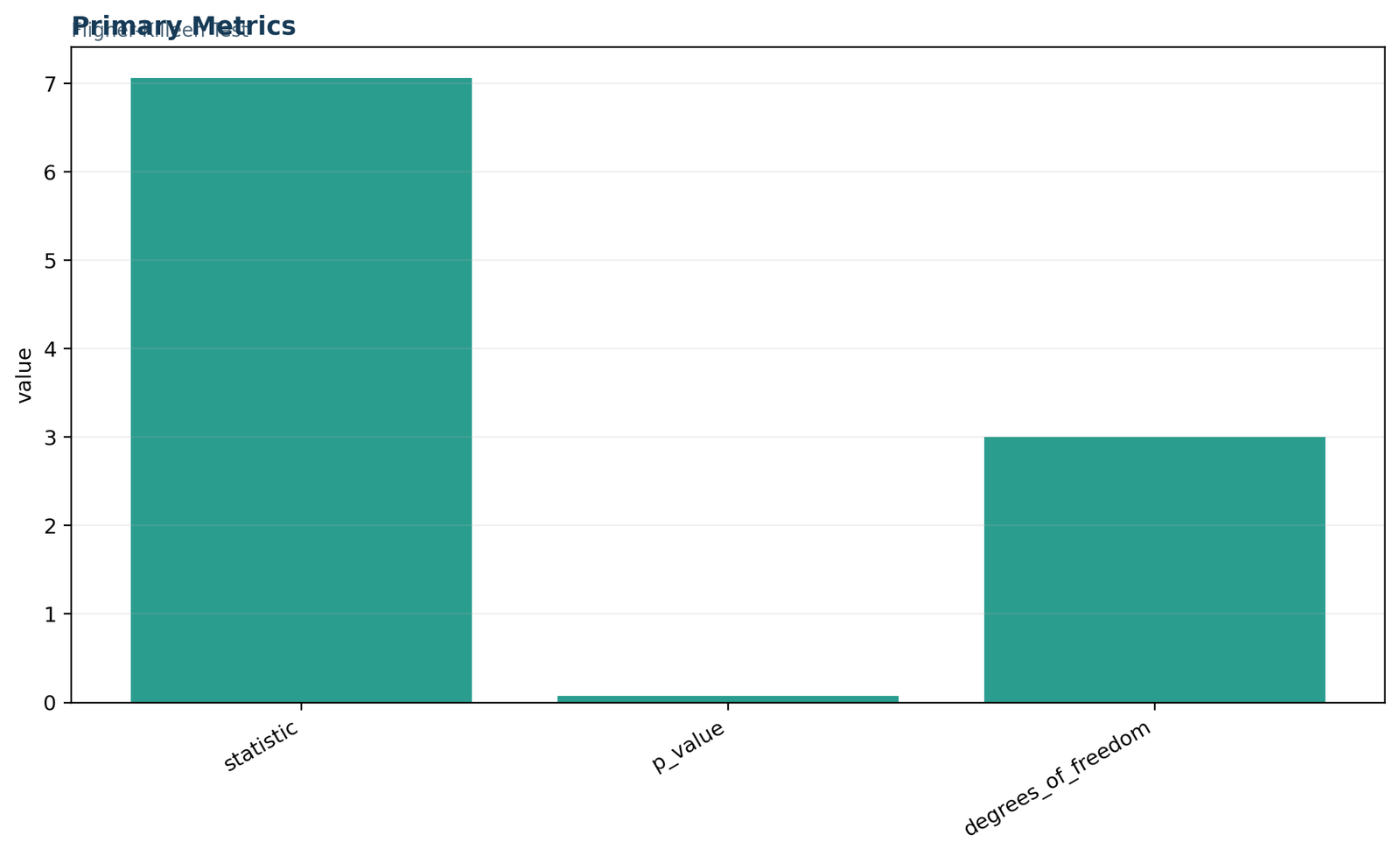
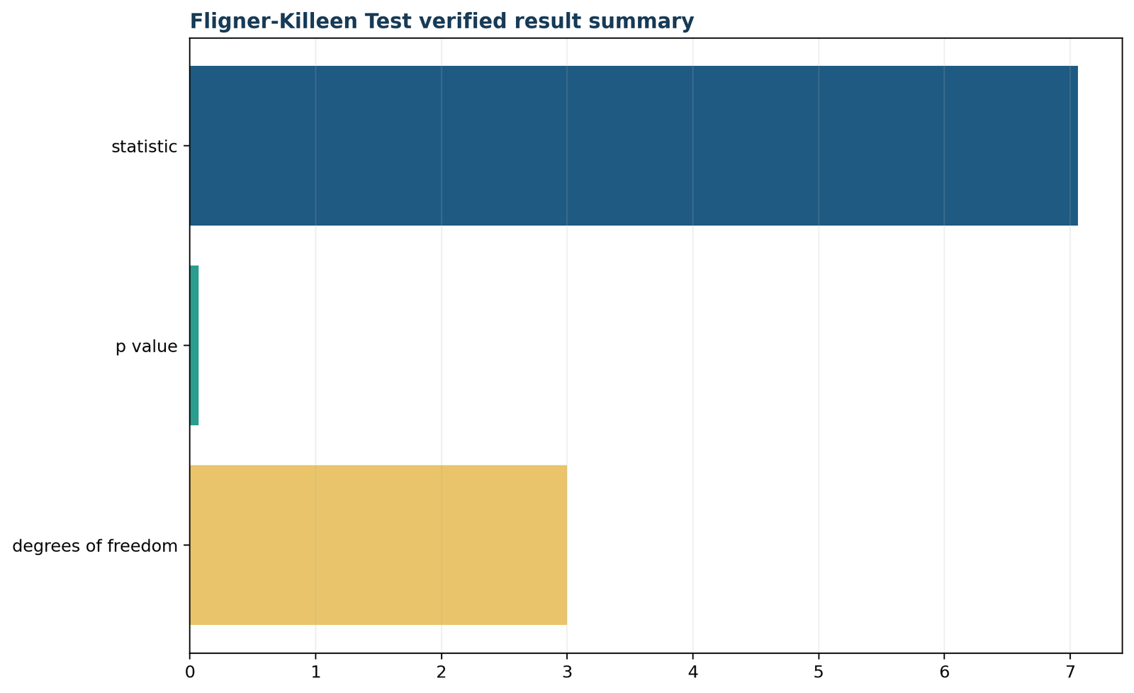
The primary-metrics panel summarizes the inferential result in one view. The Fligner Killeen test statistic is 7.0602, the reference distribution has 3 degrees of freedom, and the p-value is 0.0700. The statistic is below the .05 critical value of 7.8147, so the chart correctly classifies the result as not statistically significant.
Python chart 2: reason-group scale summary
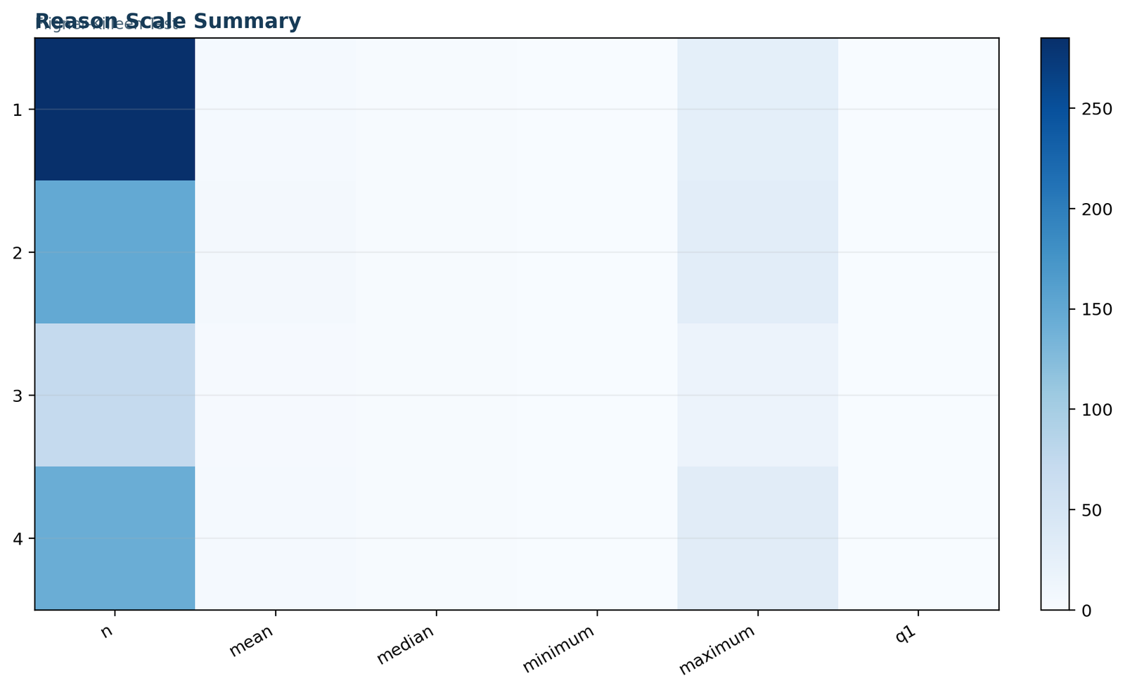
This chart compares the raw spread summaries that motivated the formal analysis. Home has the largest SD (5.579) and IQR (6), reputation also has IQR 6 and SD 4.822, course has SD 4.177, and other has the smallest SD (3.593). All group medians equal 2, keeping the descriptive focus on spread rather than location.
Python chart 3: absolute median deviations
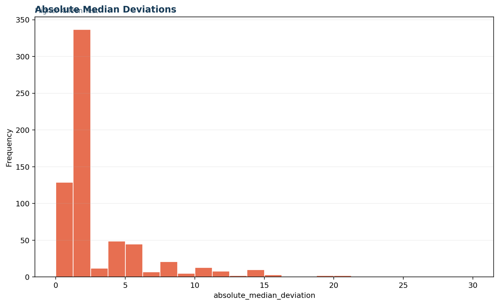
The Fligner Killeen test begins with absolute distances from each group’s median. Mean absolute deviations are 2.912 for course, 3.826 for home, 2.639 for other, and 3.406 for reputation. Home shows the largest average distance from its median, while other shows the smallest.
Python chart 4: deviation quantiles
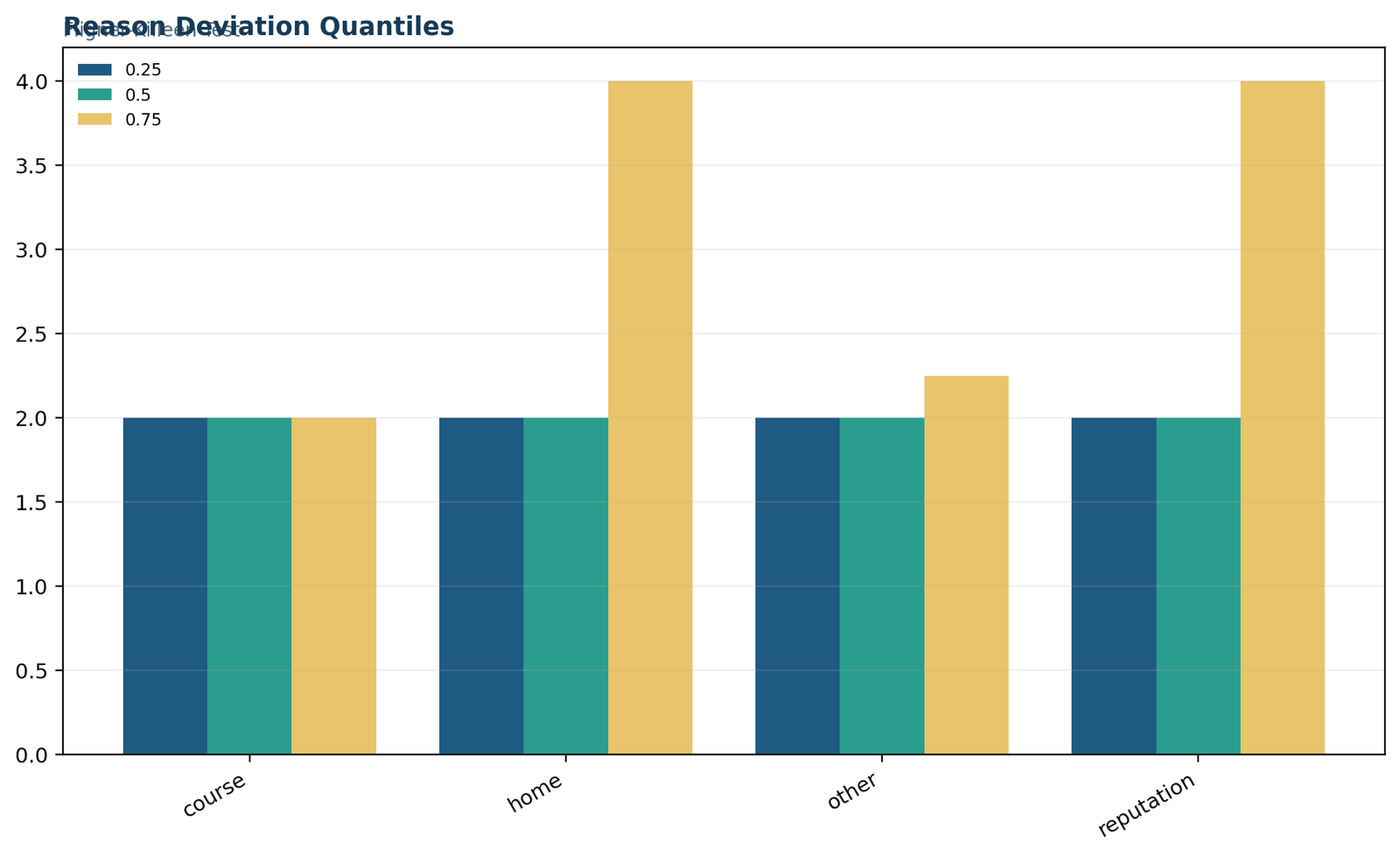
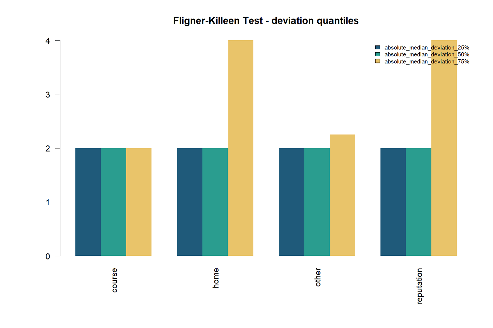
The quartile view explains the tail pattern more clearly than a single SD. The 75th percentile of absolute deviation is 2 for course, 4 for home, 2.25 for other, and 4 for reputation. The 90th percentile reaches about 10 for home, 8 for reputation, 7 for course, and 6 for other. These differences create the moderate but non-significant omnibus statistic.
Python chart 5: verified result summary
The final Python figure connects the ranked deviation calculation to the decision. It confirms χ²FK = 7.0602, df = 3, and p = 0.0700. The group patterns are visible, but the public conclusion remains that the evidence is insufficient to reject equal population scale at α = .05.
Fligner Killeen test in R: fligner.test() and chart interpretation
R provides a direct formula interface for the median-centered test.
The Fligner Killeen test in R is available through the base stats function fligner.test(). The formula syntax uses a numeric response on the left and a grouping factor on the right. The same data and group order reproduce the workbook and Python result.
df$reason <- factor(df$reason,

levels = c("course", "home", "other", "reputation"))result <- fligner.test(absences ~ reason, data = df)

result

# Fligner-Killeen:med chi-squared = 7.0602

# df = 3, p-value = 0.0700035
R chart 1: primary metrics
The R result reproduces the same statistic, degrees of freedom, and p-value. This agreement is expected because the median-centered R implementation follows the normal-score version of the Fligner Killeen test. The result remains non-significant at α = .05.
R chart 2: reason scale summary
The R scale summary shows the same descriptive ordering as Python. Home has the greatest raw spread, reputation is next, course is lower, and other is the least variable by SD and mean absolute deviation. These descriptive differences are real sample features, even though the omnibus p-value remains above .05.
R chart 3: ranked absolute median deviations
This figure focuses on the raw material used by the Fligner Killeen test. Each observation is centered on its own group median, converted to an absolute deviation, pooled with all other groups, and ranked. The higher typical deviations in home and reputation raise their mean normal scores.
R chart 4: deviation quantiles
The quantile chart shows why robust scale analysis is preferable to relying on one maximum or one outlier. Most groups share a median absolute deviation of 2, but their upper quartiles and high quantiles differ. Home has the broadest upper-deviation pattern, while other remains comparatively compact.
R chart 5: verified result summary
The final R chart confirms the complete interpretation: the sample contains visible spread differences, the Fligner Killeen test statistic is 7.0602, and the associated p-value is 0.0700. The equal-scale null is therefore not rejected at the .05 level.
fligner.test(absences ~ reason, data = df) is the most readable formula specification. A list of numeric group vectors can also be supplied. The formula and list interfaces should describe the same grouping structure and return the same result.Fligner Killeen test in SPSS
A transformation-based SPSS workflow reproduces the median-deviation normal-score statistic.
The Fligner Killeen test SPSS workflow is built from transparent data transformations: group medians, absolute deviations, pooled ranks, inverse-normal scores, and a one-way comparison of those scores. The exact final values are χ²FK = 7.0602, df = 3, and p = 0.0700.
SPSS calculation sequence
SPSS interpretation
The SPSS calculation reaches the same non-significant result as Python and R. The home and reputation groups have larger average absolute deviations than course and other, but the normal-score separation is not large enough to reject homogeneity at α = .05.
The SPSS output is best reported alongside the exact statistic and p-value rather than substituting an ordinary Kruskal–Wallis test of deviations. The defining Fligner Killeen test statistic uses inverse-normal scores of ranked deviations, not the raw deviation ranks alone.
Readers comparing software procedures may also consult ANOVA in SPSS and the guide to SPSS and R data visualization.
Fligner Killeen test Excel calculation and calculator workflow
An auditable workbook can reproduce the full statistic without hiding intermediate steps.
The Fligner Killeen test Excel workflow is also a practical Fligner Killeen test calculator. It stores the raw values separately, calculates each transformation visibly, and ends with the chi-square statistic and right-tail p-value.
Recommended workbook structure
| Sheet | Purpose |
|---|---|
| Guide | Defines the design, null hypothesis, formula, alpha, and variable coding. |
| Data_Input | Stores the original absences and reason values. |
| Working | Calculates group medians, absolute deviations, pooled ranks, probabilities, and normal scores. |
| Calculations | Summarizes group score means, score variance, χ²FK, df, and p-value. |
| Diagnostics | Records the median-centering and rank-score interpretation. |
| Reporting | Displays the final decision and cross-checks the result. |
Core Excel formulas
=MEDIAN(FILTER(absences_range,reason_range=current_reason))=ABS(absence-group_median)=RANK.AVG(deviation,all_deviations,1)=NORM.S.INV((1+rank/(N+1))/2)=CHISQ.DIST.RT(FK_statistic,k-1)Excel readers may also benefit from the guides to descriptive statistics, standard error, and confidence intervals.
Fligner Killeen test in MATLAB and SAS
The same normal-score algorithm can be reproduced when a dedicated command is not part of the preferred workflow.
The keywords Fligner Killeen test MATLAB and software-neutral implementations refer to the same six-step algorithm: median center, absolute deviation, pooled rank, inverse-normal score, group score means, and chi-square comparison.
MATLAB calculation outline
% x contains absences; g contains categorical reason labels

levels = categories(g);

N = numel(x);

d = zeros(N,1);

for i = 1:numel(levels)

idx = g == levels{i};

d(idx) = abs(x(idx) - median(x(idx),'omitnan'));

end

r = tiedrank(d);

a = norminv((1 + r/(N+1))/2);

a_bar = mean(a);

s2 = var(a,0);

% Sum n_i*(mean_i-a_bar)^2/s2 across groups

p = 1 - chi2cdf(FK, numel(levels)-1);
This outline produces the same statistic when ties, missing values, and group levels are handled consistently.
SAS calculation outline
A SAS workflow can use grouped median summaries, a DATA step for absolute deviations, PROC RANK for pooled tied ranks, the PROBIT function for normal scores, and a final grouped summary for the between-group score component. The right-tail probability is then obtained from the chi-square distribution with k − 1 degrees of freedom.
Regardless of software, the defining feature is not the syntax but the normal-score transformation of ranked absolute median deviations. A procedure that analyzes raw deviations without this transformation is not the same Fligner Killeen test.
Levene test vs Fligner Killeen test and other variance tests
Select the procedure whose robustness and assumptions match the data-generating process.
The keyword Levene test vs Fligner Killeen test reflects a common methodological decision. Both tests address homogeneity of spread, but they transform the data differently and use different reference statistics.
| Method | Main idea | Strength | Best context |
|---|---|---|---|
| Fligner Killeen test | Normal scores of ranked absolute median deviations | Strong robustness to non-normality and outliers | Skewed or heavy-tailed independent-group data |
| Levene test | ANOVA of absolute deviations from a group center | Flexible and widely available | General homogeneity testing with reasonable sample sizes |
| Brown–Forsythe test | Levene-style test centered on group medians | Robust to non-normality | Common robust variance-assumption check |
| Bartlett test | Likelihood-based comparison of sample variances | High power under normality | Approximately normal populations |
| Cochran’s C | Largest variance relative to total variance | Targets one unusually large variance | Balanced normal-theory designs |
| Hartley F-max | Largest variance divided by smallest variance | Simple diagnostic ratio | Equal sample sizes and strong normality |
| Ansari–Bradley | Symmetric rank scores for two samples | Distribution-free two-sample scale comparison | Exactly two independent groups with common location |
Fligner Killeen test vs Levene test
Levene’s test uses absolute deviations and a classical one-way comparison. The median-centered Brown–Forsythe version is robust, but the Fligner Killeen test goes further by ranking deviations and converting the ranks to normal scores. In strongly non-normal data, that rank transformation can reduce sensitivity to extreme raw magnitudes.
See the dedicated Levene test and Brown–Forsythe test guides for their formulas and interpretation.
Fligner Killeen test vs Bartlett test
Bartlett’s test is efficient when each group is normally distributed, but it can respond strongly to non-normality. The Fligner Killeen test sacrifices direct variance-likelihood modeling in exchange for robustness. For skewed absence counts with many ties and outliers, the robust rank-based approach is the more natural primary analysis.
Related comparisons include Cochran’s C test, Hartley F-max, and broader ANOVA assumption diagnostics.
Diagnostics, NA results, and common Fligner Killeen test errors
Most software problems arise from missing values, invalid grouping variables, or a mismatch between the intended and actual formula.
Searches such as why does Fligner Killeen test have NA, Fligner Killeen test p value is NA, and all group levels must be finite Fligner Killeen test usually point to data-handling problems rather than a mysterious statistical result.
Why the p-value may be NA
“All group levels must be finite”
This R error commonly appears when the grouping input is not a valid factor or finite numeric grouping vector in the default interface. Converting the grouping column to a factor and checking missing labels resolves the structural problem:
df <- subset(df, is.finite(absences) & !is.na(reason))

df$reason <- factor(df$reason)

fligner.test(absences ~ reason, data = df)
The phrase refers to the group levels, not only the numeric response. A character vector passed through the wrong interface can therefore trigger the message even when every outcome value is finite.
Python missing values
SciPy’s nan_policy="propagate" returns a missing result when NaN values are present in the analyzed slice. nan_policy="omit" removes missing observations, provided enough data remain.
R missing values
The formula interface uses the configured na.action. The number of retained observations and group counts should be checked after case deletion.
Excel missing values
Blank cells, text values, and formula-generated empty strings need consistent treatment before group medians, ranks, and normal scores are calculated.
Useful supporting diagnostics include skewness, kurtosis, skewness and kurtosis checks, and percentiles and quartiles.
How to report the Fligner Killeen test in APA style
A complete result includes the design, statistic, degrees of freedom, exact p-value, decision, and descriptive spread pattern.
A strong Fligner Killeen test interpretation should not consist of “p > .05” alone. Readers need to know which outcome and groups were analyzed, why the robust test was used, and what the group spread summaries showed.
APA-style result
A Fligner–Killeen test was conducted to compare the variability of student absences across four school-choice reason groups. The homogeneity-of-scale result was not statistically significant, χ2FK(3) = 7.06, p = .070. The home group showed the largest sample standard deviation (SD = 5.58), followed by reputation (SD = 4.82), course (SD = 4.18), and other (SD = 3.59), but the evidence was insufficient to reject equal population scale at α = .05.
Compact technical report
Fligner Killeen test: χ²FK(3, N = 649) = 7.0602, p = 0.0700. Median-centered absolute deviations were ranked and transformed using Fligner normal scores. The equal-scale null was not rejected.
Reporting checklist
Fligner Killeen test PDF, Excel, and software downloads
Each download corresponds to the same absences-by-reason analysis.
Python reportVerified Python calculation, tables, and charts.Open Python PDF
R reportR fligner.test() result and matching interpretation.Open R PDF
SPSS outputTransformation-based SPSS analysis and verified result.Open SPSS PDF
Excel workbookAuditable median deviations, ranks, normal scores, and final statistic.Open Excel workbook
Fligner Killeen test FAQs
Answers to the most common questions about assumptions, interpretation, software, and errors.
What is the Fligner Killeen test?
The Fligner Killeen test is a robust k-sample test of equal population variance or scale. It uses normal scores derived from ranked absolute deviations from group medians.
What is the Fligner Killeen test null hypothesis?
The null hypothesis states that all groups have the same population variance or scale. The alternative states that at least one group differs.
Does the Fligner Killeen test require normality?
No. Its rank-based construction makes it robust to departures from normality, which is a major reason to prefer it over Bartlett’s test for skewed or heavy-tailed data.
How do I interpret a non-significant Fligner Killeen test?
A non-significant result means that the data do not provide sufficient evidence of unequal population scale at the selected significance level. It does not prove exact equality.
What does p = 0.070 mean in this example?
At α = .05, p = .070 is not statistically significant. The equal-scale null is not rejected, although the descriptive spread differences remain visible.
How many groups can the Fligner Killeen test compare?
It can compare two or more independent groups. The final chi-square reference uses k − 1 degrees of freedom.
Is the Fligner Killeen test the same as Levene’s test?
No. Both test homogeneity of spread, but Levene’s test analyzes absolute deviations directly, while the Fligner Killeen test ranks the deviations and applies inverse-normal scores.
When is the Fligner Killeen test better than Bartlett’s test?
It is usually preferable when normality is doubtful, the data are skewed or heavy-tailed, or extreme values could distort a normal-theory variance test.
Can the Fligner Killeen test be used with unequal sample sizes?
Yes. Unequal group sizes are allowed, as demonstrated by the sample sizes 285, 149, 72, and 143 in this example.
Why does fligner.test return NA?
Common causes include missing or non-finite outcome values, invalid group labels, empty groups after filtering, insufficient usable observations, or a degenerate score variance.
What does “all group levels must be finite” mean?
It means that the grouping input supplied to the R default interface is not a valid finite grouping vector. Converting the grouping column to a factor and removing missing labels usually resolves the structure.
How is the Fligner Killeen test run in Python?
Use scipy.stats.fligner with one array per group and median centering. The worked result is statistic = 7.0602 and p = 0.0700.
How is the Fligner Killeen test run in R?
Use fligner.test(outcome ~ group, data = data_frame). In this example, the formula is fligner.test(absences ~ reason, data = df).
Can the Fligner Killeen test be calculated in Excel?
Yes. Excel can calculate group medians, absolute deviations, tied ranks, inverse-normal scores, group score means, the statistic, and the chi-square p-value.
Does a significant result identify which groups differ?
No. The test is omnibus. A significant result indicates that at least one group scale differs, but planned pairwise scale comparisons are needed to locate the difference.
What center does the standard test use?
The standard R median version centers observations on their group medians. SciPy also permits mean or trimmed-mean centering, but the selected version should be reported.
Why are ties important in this analysis?
Absence counts contain many repeated values. Tied absolute deviations receive average ranks, which then determine the normal scores and final statistic.
What should accompany the test in a research report?
Report group sample sizes, medians, SDs or IQRs, the center used, χ²FK, df, exact p-value, and a careful population-scale interpretation.
Related statistical guides
Internal resources for variance testing, assumptions, descriptive analysis, and interpretation.