
Variance Components, Random-Level Means, ICC, F Test and Residual Diagnostics
Random Effects ANOVA: Formula, Interpretation, SPSS, Python, R and Excel Guide
Random Effects ANOVA is used when factor levels are treated as a sample from a larger population of possible levels. Instead of only comparing the listed groups as fixed categories, the model estimates how much variation is attributable to the random factor and how much remains as residual error. In this worked example, studytime is treated as a random factor level for G3 final grade. The model finds a significant random-level effect, a between-level variance component of 1.0375, a residual variance component of 9.7646, and an intraclass correlation of 0.0960.
Quick Answer: Random Effects ANOVA Result
The worked Random Effects ANOVA compares G3 final grade across studytime levels treated as sampled random levels. The F test for random-level variance is significant, with F = 15.876, df1 = 3, df2 = 645, and p = 5.706e-10. The observed F statistic is far above the critical value of 2.619, so the random-level differences are statistically supported.
The variance components show that the between-random-level variance is 1.0375, while the residual error variance is 9.7646. The intraclass correlation is ICC = 0.0960, meaning about 9.6% of total model variance is attributable to differences between the random studytime levels, while about 90.4% remains within levels as residual error.
Final interpretation: Studytime levels show statistically significant random-level differences in G3, but most variation remains within the levels. The ICC of 0.0960 means random studytime levels account for about 9.6% of total model variance, while residual individual-level variation accounts for about 90.4%.
Important reporting point: Random Effects ANOVA is not the same as treating studytime as a fixed factor. A fixed-effects ANOVA focuses on the exact levels in the dataset. A random-effects ANOVA estimates how much variance is attributable to levels sampled from a larger possible population of levels.
Table of Contents
- What Is Random Effects ANOVA?
- Random Effects ANOVA Formula
- Random Effects ANOVA Hypotheses
- Dataset and ANOVA Variables Used
- SPSS Output Interpretation for Random Effects ANOVA
- Python Chart-by-Chart Interpretation
- R Chart-by-Chart Validation
- SPSS, R, Python and Excel Workflows
- Code Blocks for Random Effects ANOVA
- APA Reporting Wording
- Common Mistakes
- When to Use Random Effects ANOVA
- Downloads and Resources
- Related Guides
- FAQs
What Is Random Effects ANOVA?
Random Effects ANOVA is an ANOVA model where the factor levels are treated as a random sample from a larger population of possible levels. The goal is not only to compare the observed levels, but to estimate variance components that describe how much outcome variation belongs to the random factor and how much remains as residual error.
In a fixed-effects model, the studytime levels would be interpreted as the exact four categories of interest. In a random-effects model, those levels are treated as sampled levels used to estimate a broader between-level variance component. This is useful when the researcher wants a variance estimate rather than only a list of mean differences.
In this worked example, the random-level variance is 1.0375, the residual variance is 9.7646, and the ICC is 0.0960. The ICC is the most compact practical summary because it shows the share of total variance attributable to random levels.
Simple definition: Random Effects ANOVA estimates how much variation is due to random factor levels. In this example, studytime levels explain about 9.6% of G3 variance, while residual error explains about 90.4%.
Random Effects ANOVA connects naturally with One Way ANOVA, Fixed Effects ANOVA, Nested ANOVA, Mixed ANOVA, Factorial ANOVA, ANOVA Effect Size, F Distribution, Eta Squared, Omega Squared, and ANOVA Assumptions.
Random Effects ANOVA Formula
A simple one-way random effects model separates an observed score into a grand mean, a random level effect, and residual error.
Here, Yij is the observed G3 score for student i in random level j. The term μ is the grand mean. The random level effect aj represents how much a sampled level differs from the grand mean. The residual term eij represents individual variation inside each random level.
Variance Components
The model estimates two main variance components. The between-level component is σ²level. The residual component is σ²error. In this output, the between-level component is 1.0375, and the residual component is 9.7646.
Intraclass Correlation Formula
Using the values in this report, ICC = 1.0375 / (1.0375 + 9.7646) = 0.0960. This means 9.6% of the model variance is between random levels and 90.4% is residual error.
F Test Formula
The F distribution chart reports F = 15.876, critical F = 2.619, df1 = 3, df2 = 645, and p = 5.706e-10. This means the random-level mean variation is much larger than expected under a no-between-level-variance model.
| Quantity | Value | Meaning | Interpretation |
|---|---|---|---|
| Between random levels variance | 1.0375 | Variation attributable to random factor levels. | There is measurable between-level variation. |
| Residual variance | 9.7646 | Variation remaining within levels. | Most variation remains inside levels. |
| ICC | 0.0960 | Between-level share of total variance. | About 9.6% of variance is between levels. |
| 1 − ICC | 0.9040 | Residual share of total variance. | About 90.4% of variance is within levels. |
| Observed F | 15.876 | Between-level MS compared with residual MS. | Random-level effect is statistically supported. |
Random Effects ANOVA Hypotheses
The key hypothesis in a random effects ANOVA focuses on the between-level variance component. Instead of asking only whether fixed means differ, the random-effects question asks whether the population variance among levels is greater than zero.
| Statement | Statistical Meaning | Plain Interpretation |
|---|---|---|
| Null hypothesis | σ²level = 0 | The random factor levels do not explain meaningful variation in G3. |
| Alternative hypothesis | σ²level > 0 | The random factor levels explain some variation in G3. |
| Decision rule | Reject when p < .05 | The reported p-value is far below .05. |
Decision for this example: The random-level variance is statistically supported. The F test gives F = 15.876 and p = 5.706e-10. The ICC shows the practical size: about 9.6% of the model variance is attributable to random levels.
Dataset and ANOVA Variables Used
The worked example uses student performance data. The dependent variable is G3 final grade. The random factor is studytime, treated as a sampled random-level factor for the purpose of variance-component explanation.
| Variable | Role | What It Represents | Why It Matters |
|---|---|---|---|
| G3 | Dependent variable | Final grade outcome. | The numeric score whose variance is decomposed. |
| studytime | Random factor | Four sampled levels. | Used to estimate between-level variance. |
| Random-level means | Descriptive output | Mean G3 for each level. | Shows direction of between-level differences. |
| Residuals | Model error | Observed G3 minus level mean. | Used for within-level variance and diagnostics. |
Random-Level Mean Pattern
| Random Level | Approximate Mean G3 | Visual Pattern | Interpretation |
|---|---|---|---|
| Level 1 | About 10.84 | Lowest bar and lowest central boxplot position. | Lowest random-level mean. |
| Level 2 | About 12.09 | Higher than level 1. | Middle random-level mean. |
| Level 3 | About 13.23 | Highest mean with relatively tighter interval. | Highest random-level mean. |
| Level 4 | About 13.06 | High mean but wider uncertainty. | High random-level mean with smaller sample support. |
The mean pattern explains why the F test is significant. Level 1 is visibly lower than levels 3 and 4. However, the variance component chart and ICC show that most outcome variation still remains inside the levels rather than between them.
For background, review Descriptive Statistics, Mean Median and Mode, Standard Deviation, Variance, Confidence Interval, P Value, and Null and Alternative Hypothesis.
SPSS Output Interpretation for Random Effects ANOVA
The SPSS output should be read as a variance-component model rather than only a mean-comparison table. The most important parts are the random factor, the variance component estimates, the intraclass correlation interpretation, the F test and the residual diagnostics.
SPSS Reading Order
| SPSS Output Area | What to Read | Why It Matters |
|---|---|---|
| Model specification | G3 as dependent variable and studytime as random factor. | Confirms that the analysis is random-effects, not only fixed-effects. |
| Random-level means | Means and confidence intervals for studytime levels. | Shows the observed direction of level differences. |
| Variance components | Between-level and residual variance estimates. | Shows how total model variation is divided. |
| ICC calculation | Between variance divided by total variance. | Shows the proportion of variance attributable to random levels. |
| F test | F statistic, df and p-value. | Tests whether random-level differences are statistically supported. |
| Residual diagnostics | Histogram and Q-Q plot. | Shows whether residual shape is approximately acceptable. |
SPSS Variance Component Summary
| Component | Estimate | Share | Interpretation |
|---|---|---|---|
| Between random levels | 1.0375 | 9.6% | Studytime levels account for a small but real share of model variance. |
| Residual error | 9.7646 | 90.4% | Most G3 variation remains within the random levels. |
| Total model variance | 10.8021 | 100% | Sum of between-level and residual variance. |
SPSS F Test Summary
| Statistic | Value | Interpretation |
|---|---|---|
| Observed F | 15.876 | Between-level variation is much larger than residual expectation. |
| Critical F | 2.619 | The observed statistic is far beyond the .05 decision boundary. |
| df1 | 3 | Numerator degrees of freedom for four levels. |
| df2 | 645 | Residual degrees of freedom. |
| p-value | 5.706e-10 | Reject the no-between-level-variance null. |
The SPSS result supports a statistically significant random-level effect, but the variance share must be interpreted carefully. The random factor accounts for 9.6% of model variance, which is meaningful but smaller than the residual share. Therefore, the analysis supports a random-level effect without claiming that studytime levels explain most grade variation.
SPSS interpretation summary: The random-level effect is statistically significant, F(3, 645) = 15.876, p = 5.706e-10. The between-level variance is 1.0375 and the residual variance is 9.7646. ICC = 0.0960, so about 9.6% of variance is attributable to random levels.
Python Chart-by-Chart Interpretation
The Python chart sequence explains Random Effects ANOVA through random-level means, distributions, variance components, variance share, F distribution, ICC, residual histogram and residual Q-Q diagnostics.
Python Chart 1: Random-Level Means with 95% Confidence Intervals
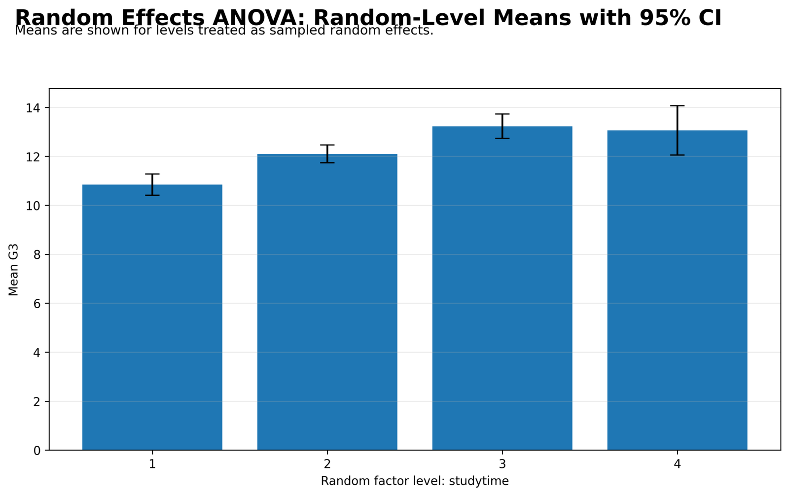
This chart shows the mean G3 value for each random studytime level. Level 1 is lowest at about 10.84, level 2 is higher at about 12.09, level 3 is highest at about 13.23, and level 4 remains high at about 13.06.
The mean pattern explains why the random-level F test is significant. Level 1 is visibly below levels 3 and 4. Level 4 has the widest interval, so its mean is less precise than the larger levels, but it still remains in the high range.
Python Chart 2: Distribution by Random Level
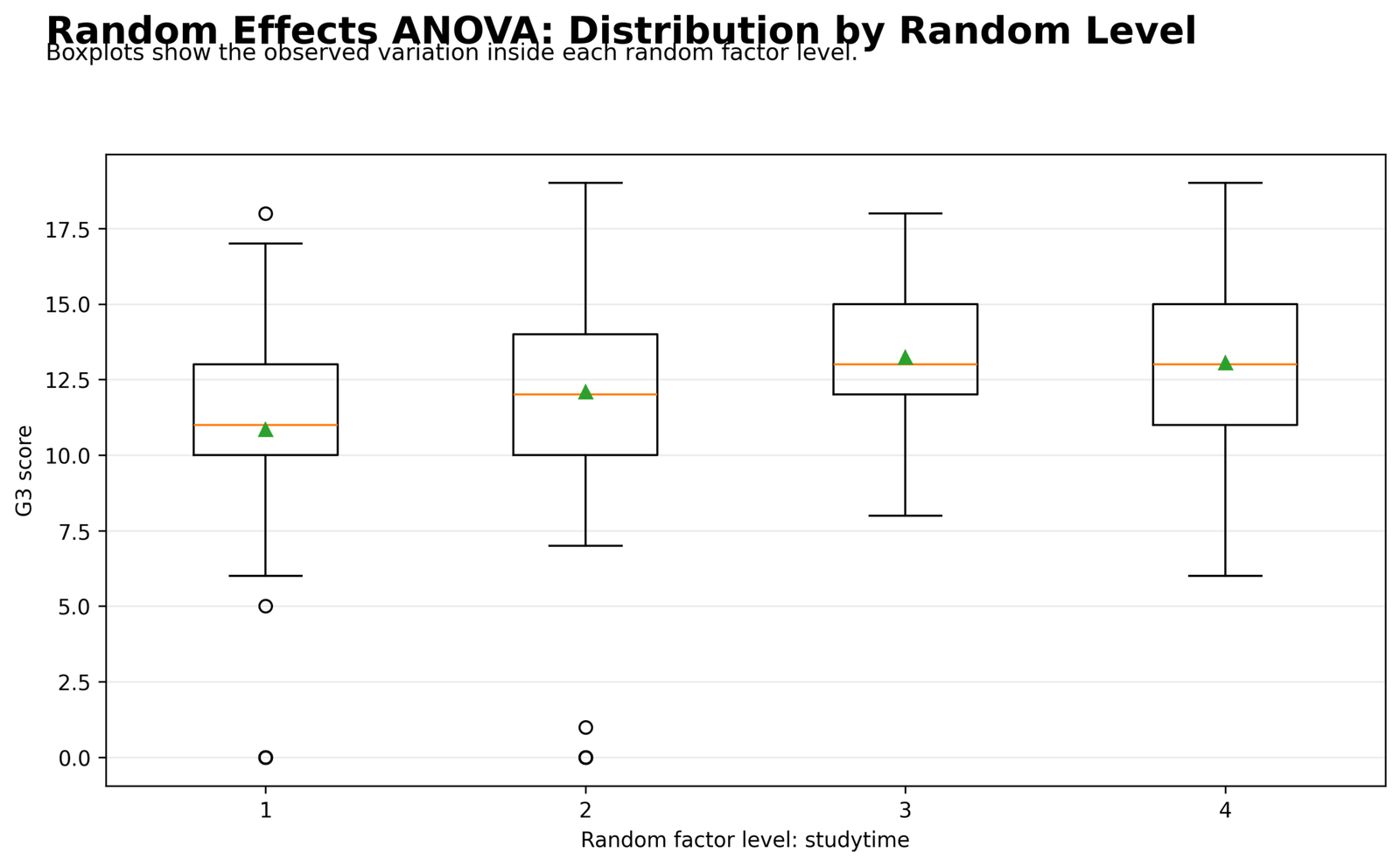
The boxplots show that level 1 has the lowest center, while levels 3 and 4 are centered higher. Level 2 sits between the lower and higher random levels.
The chart also shows strong within-level variation, including low values in levels 1 and 2. This supports the ICC interpretation: there are real level differences, but most of the total variation still occurs within levels rather than between levels.
Python Chart 3: Variance Components
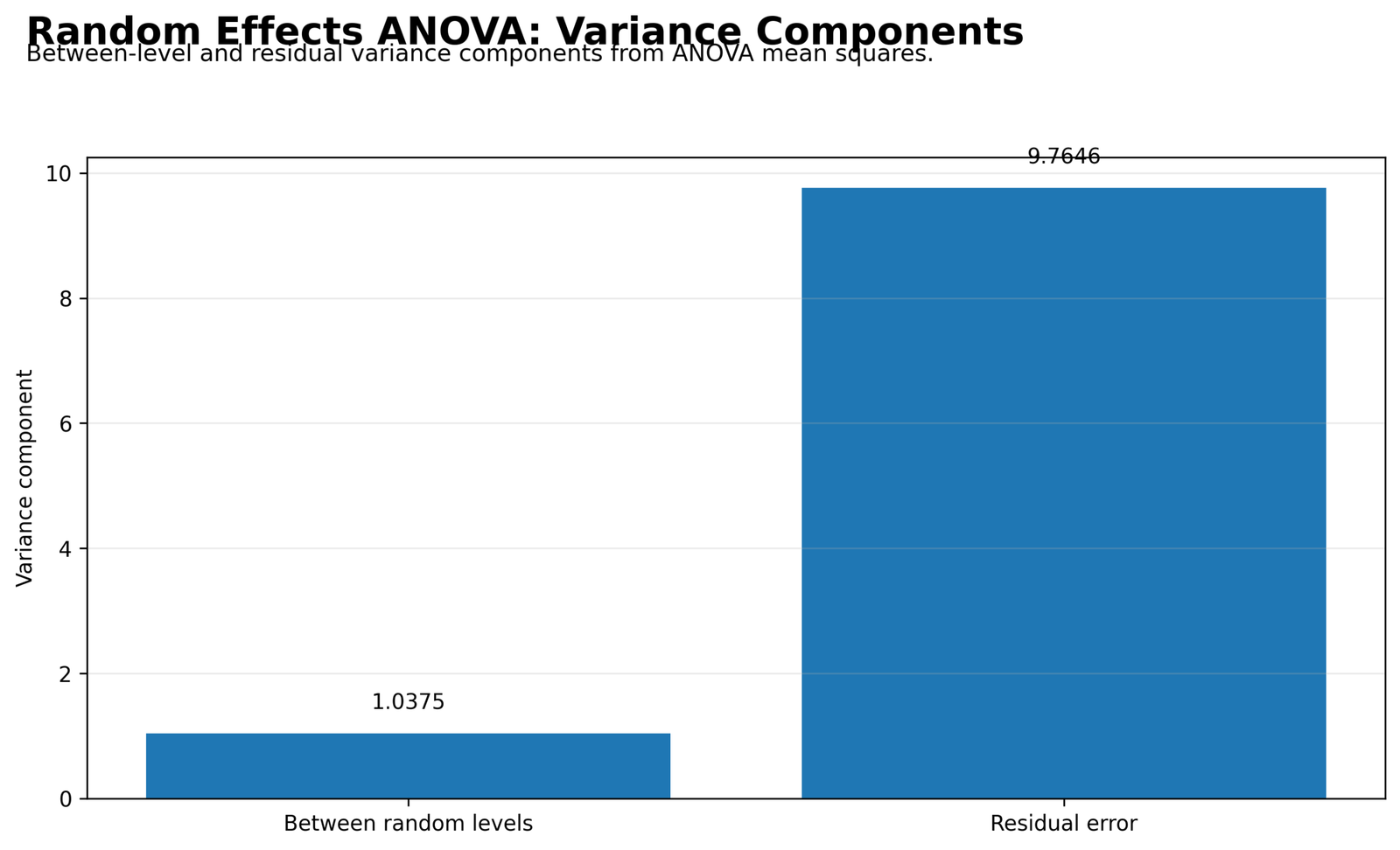
The variance components chart shows a between-random-level component of 1.0375 and a residual error component of 9.7646. The residual component is much larger than the between-level component.
This is the central Random Effects ANOVA message. The random factor contributes measurable variation, but individual residual variation dominates the model. The model therefore supports a random-level effect without overstating its practical size.
Python Chart 4: Variance Component Share
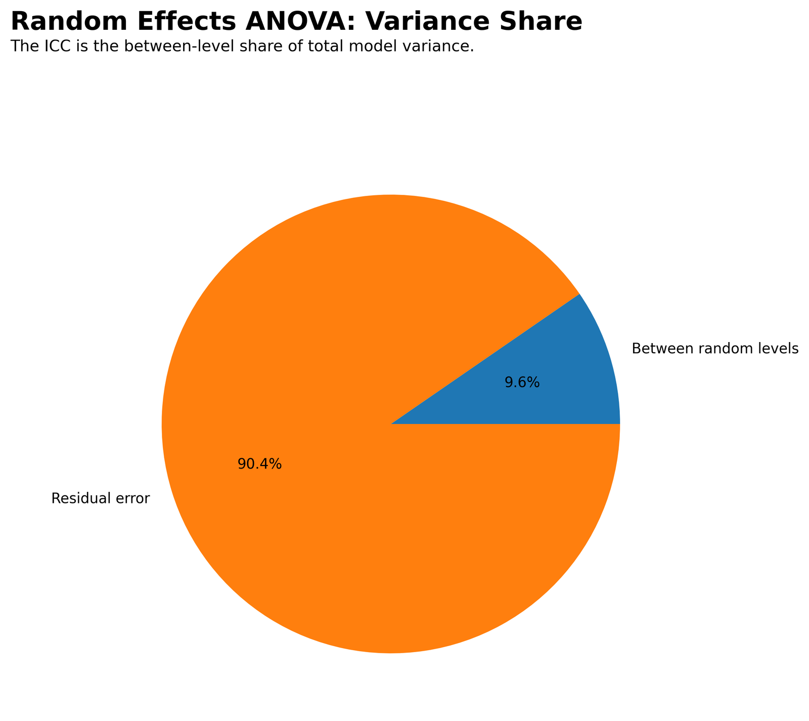
The variance share chart converts the variance components into percentages. Between random levels account for 9.6% of total model variance, while residual error accounts for 90.4%.
This chart is useful for nontechnical reporting because it communicates the ICC result visually. The random factor matters, but most variation remains within levels, so additional predictors or individual-level variables would still be needed to explain more of G3.
Python Chart 5: F Test for Random-Level Variance
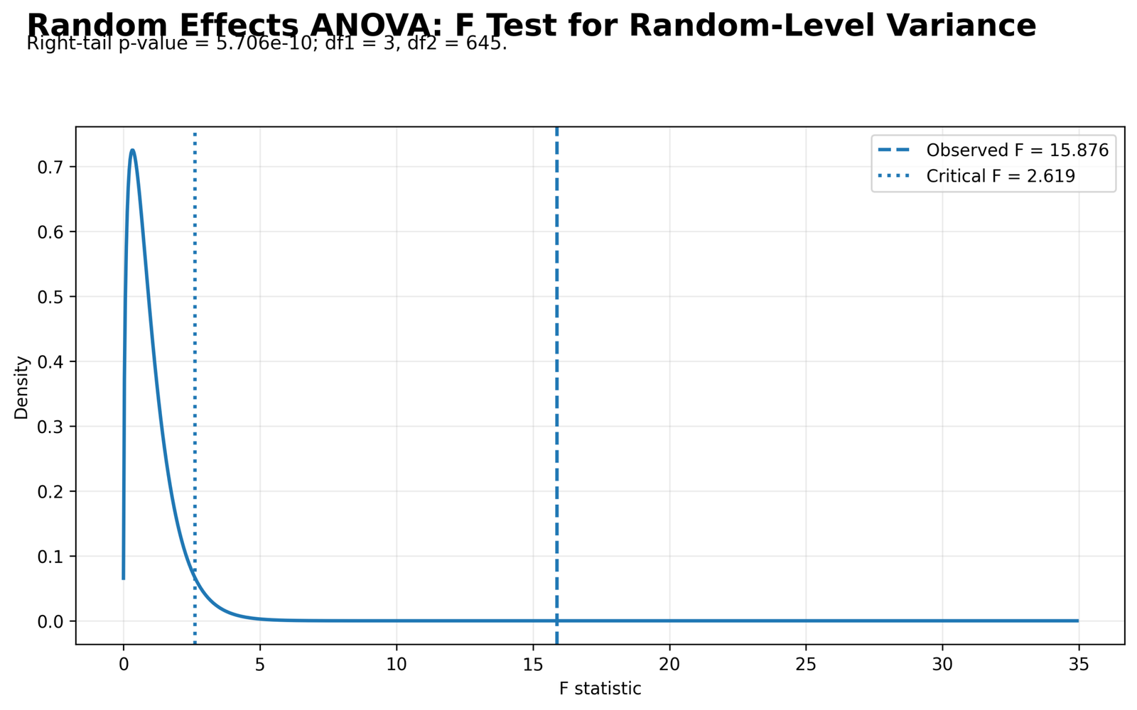
The F distribution chart shows F = 15.876, critical F = 2.619, df1 = 3, df2 = 645, and p = 5.706e-10. The observed F line is far to the right of the critical F line.
The decision is clear. The no-between-level-variance null is rejected. The random levels differ more than expected by residual variation alone.
Python Chart 6: Intraclass Correlation Summary
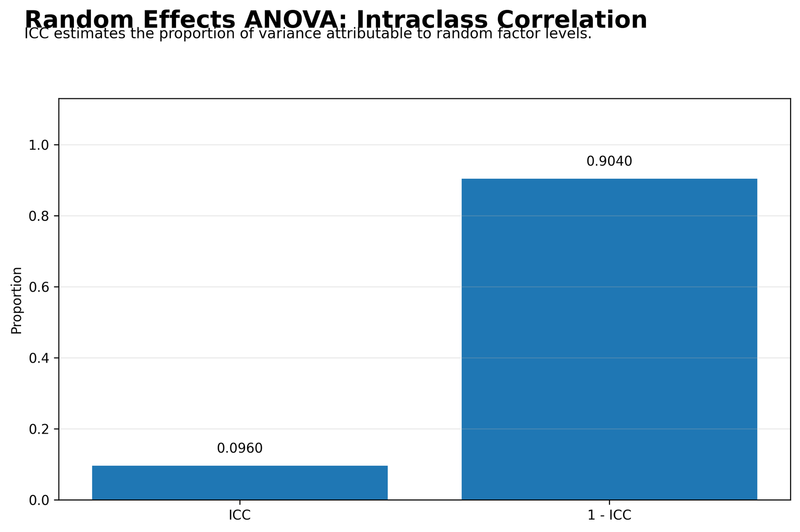
The ICC chart reports ICC = 0.0960 and 1 − ICC = 0.9040. This means 9.6% of variance belongs to random-level differences, while 90.4% belongs to residual within-level variation.
This is the best practical summary of the random effects model. The F test confirms significance, while the ICC explains the size of the random-level contribution.
Python Chart 7: Residual Histogram
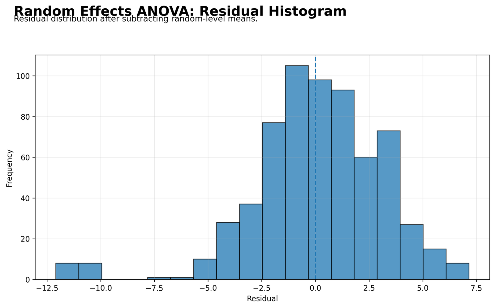
The residual histogram is centered close to zero, which is expected after subtracting random-level means. Most residuals fall in the central range, but the distribution has a noticeable lower tail with values around -10 to -12.
The histogram supports a cautious assumption statement. The residual pattern is informative, but it is not perfectly normal because of low-score residual cases. This does not erase the random-level effect, but it should be reported in the diagnostics section.
Python Chart 8: Residual Q-Q Plot
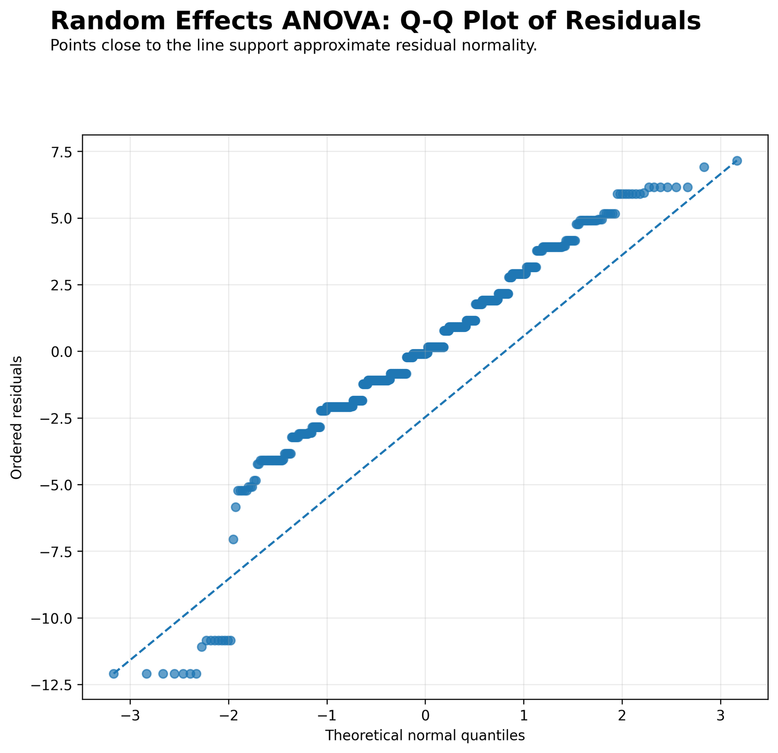
The Q-Q plot shows that the residuals do not follow the reference line perfectly. The lower tail departs strongly, and the ordered residuals show a stepped pattern because the grade outcome is discrete.
The diagnostic conclusion is balanced. The random-level effect is statistically significant, but residual normality is approximate rather than ideal. The final report should mention the lower-tail departure and the discrete grade structure.
R Chart-by-Chart Validation
The R validation charts repeat the same Random Effects ANOVA workflow in a second software environment. They confirm the random-level mean pattern, boxplot structure, variance components, variance share, F decision, ICC summary, residual histogram and Q-Q diagnostics.
R Chart 1: Random-Level Means with 95% Confidence Intervals
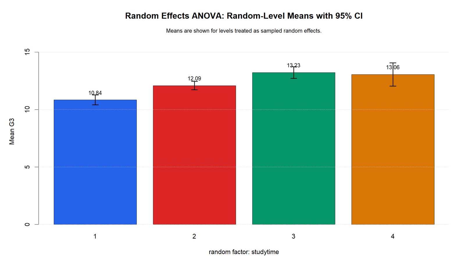
The R random-level mean chart confirms the Python pattern. Level 1 is lowest, level 2 is higher, and levels 3 and 4 are in the highest range.
This validation strengthens the interpretation because the same mean structure appears in both workflows. The random-level effect is not a graphing artifact.
R Chart 2: Distribution by Random Level
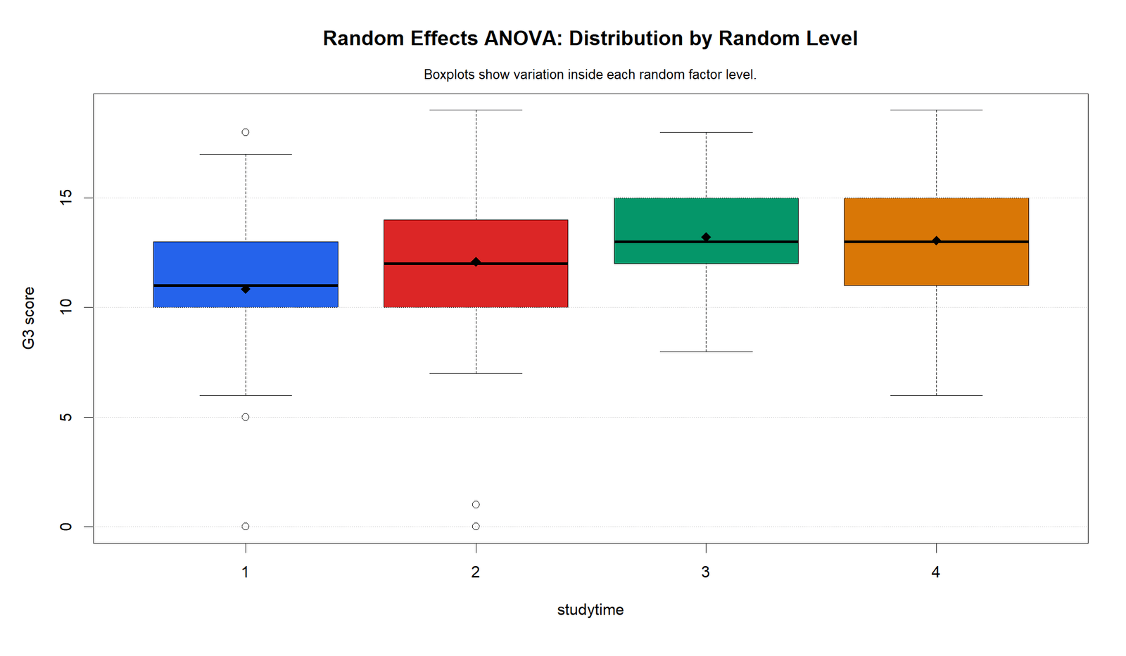
The R boxplots confirm that higher random levels have higher central G3 values, while level 1 remains the lowest. The within-level spread remains visible across all groups.
This supports the same ICC interpretation. Random levels explain part of the variation, but within-level variation remains much larger.
R Chart 3: Variance Components
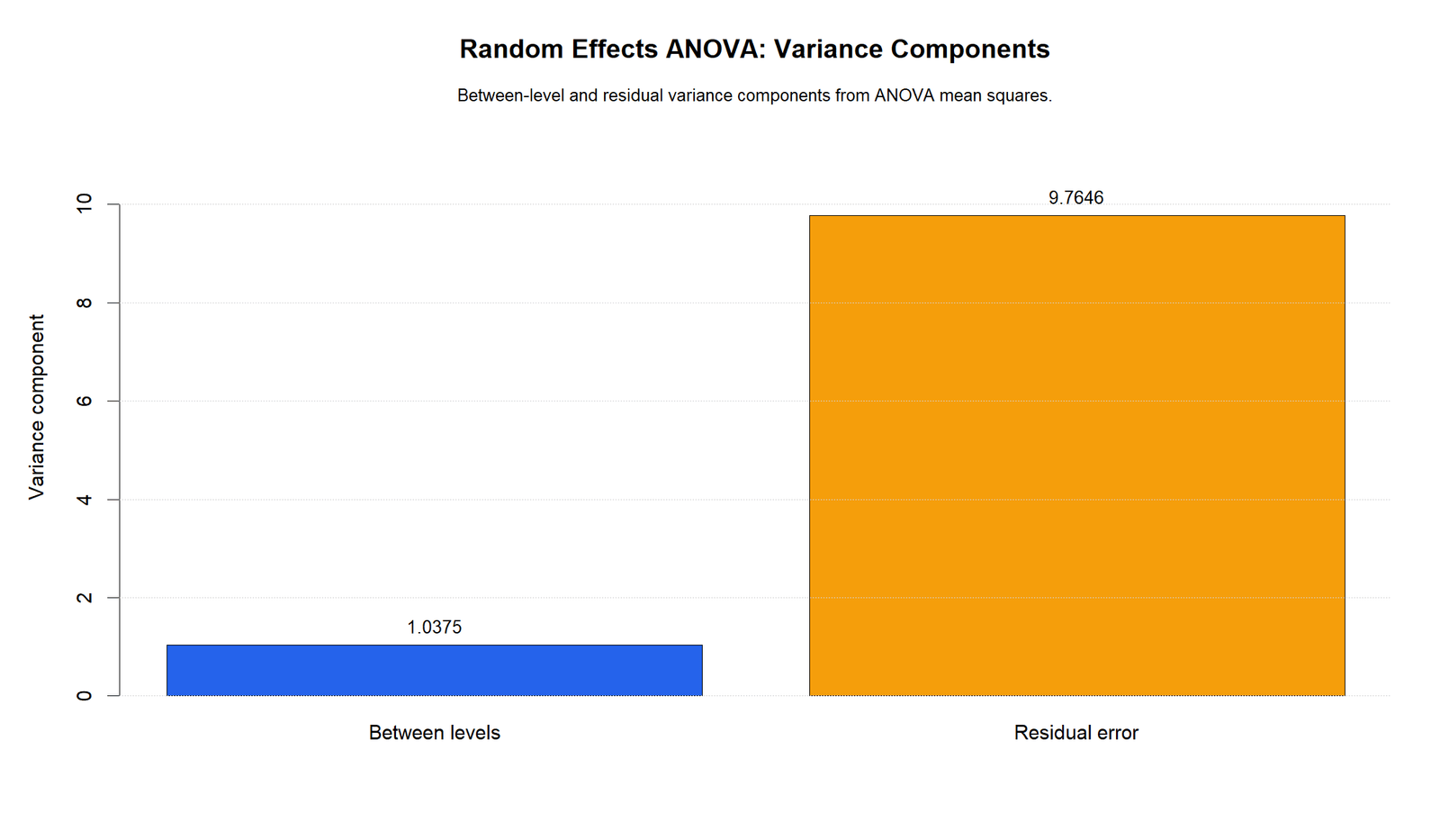
The R variance component chart confirms the same estimates: the between-random-level component is much smaller than the residual error component.
This means the practical conclusion is stable across Python and R. The model detects between-level variation, but most variation remains residual.
R Chart 4: Variance Component Share
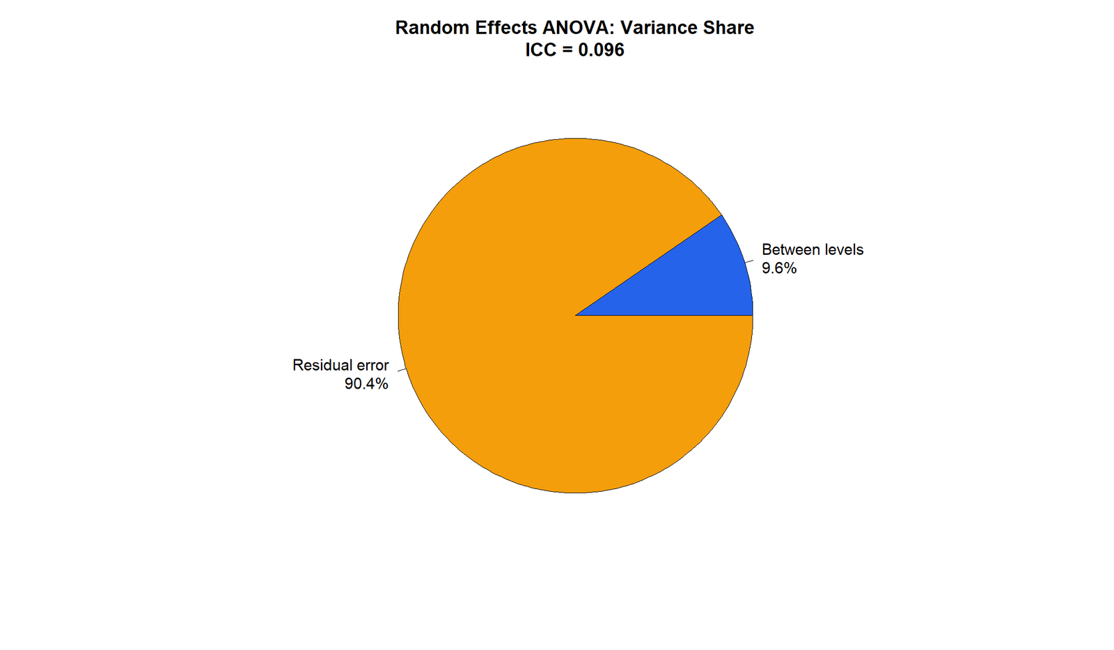
The R variance share chart confirms that the random factor accounts for about 9.6% of total model variance and residual error accounts for about 90.4%.
This validates the ICC-based interpretation. The random factor matters, but it is not the dominant source of G3 variation.
R Chart 5: F Test for Random-Level Variance
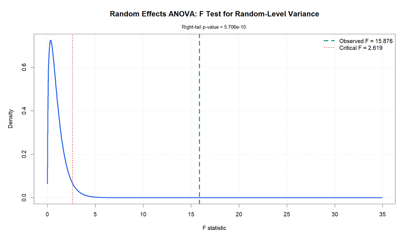
The R F distribution chart confirms that the observed F statistic is far beyond the critical F value. The same p-value decision is supported.
The chart validates the inferential result: random-level differences are statistically significant, not a borderline outcome.
R Chart 6: Intraclass Correlation Summary
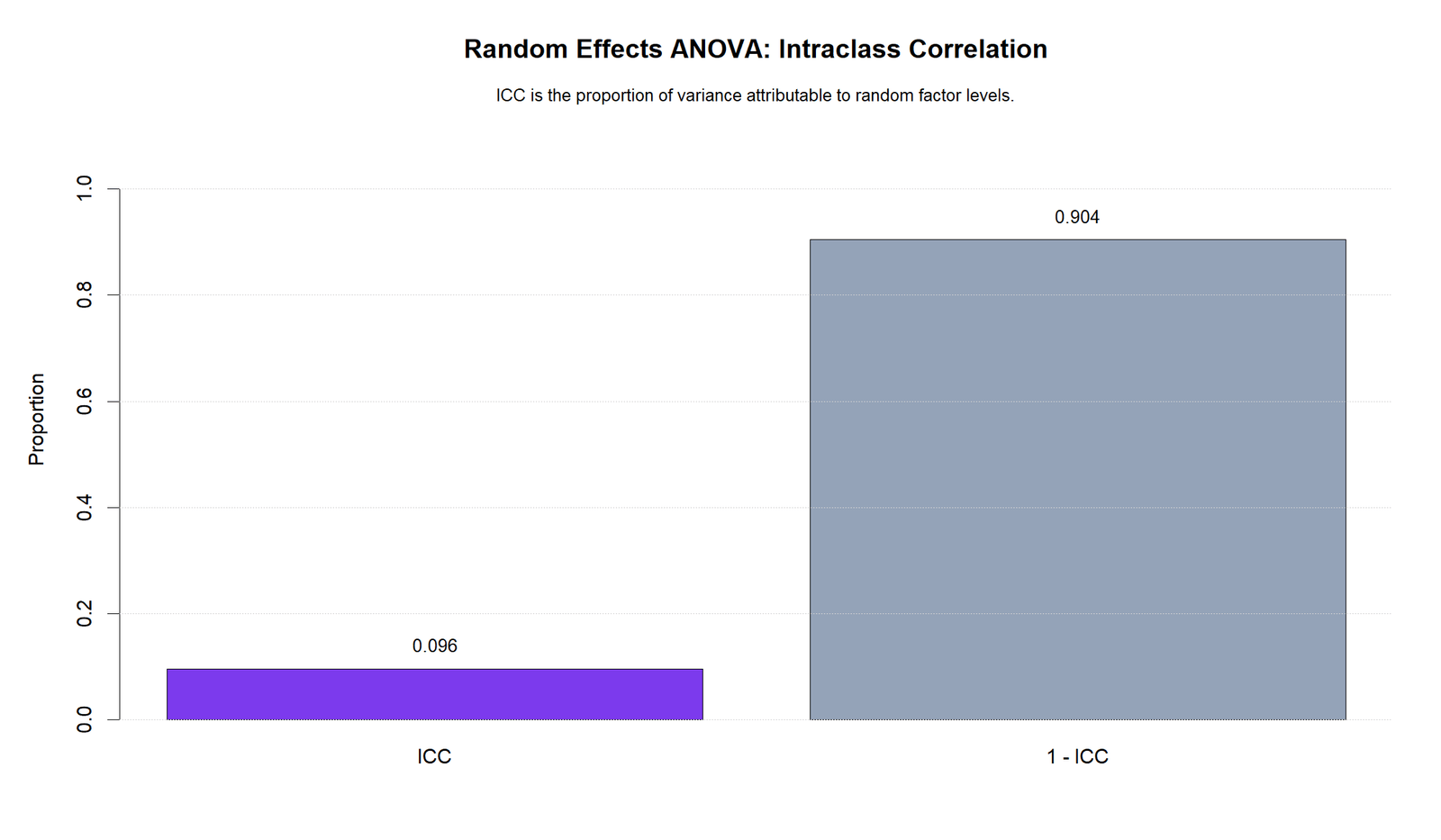
The R ICC chart confirms ICC = 0.0960. The 1 − ICC value remains 0.9040.
This confirms the main practical conclusion: random-level differences explain a real but modest portion of G3 variance.
R Chart 7: Residual Histogram
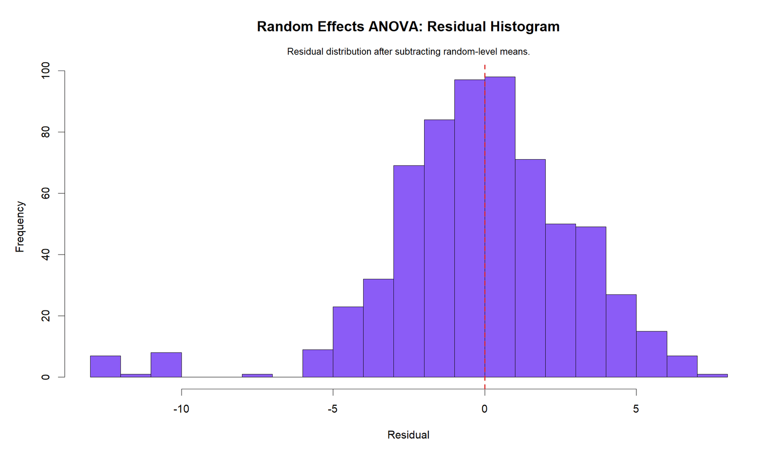
The R residual histogram confirms the same residual shape. Most residuals are near zero, but the lower tail remains visible.
This supports the same diagnostic statement as the Python output. The residual distribution is not perfectly normal, mainly because of low residual values.
R Chart 8: Residual Q-Q Plot
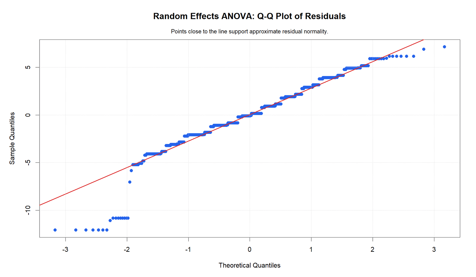
The R Q-Q plot confirms the lower-tail departure and stepped residual pattern. The central residuals are closer to the line than the extreme lower values.
This validation completes the diagnostic message. The random effect is significant, but residual normality should be described as approximate rather than perfect.
SPSS, R, Python and Excel Workflows for Random Effects ANOVA
The same Random Effects ANOVA workflow can be reproduced in SPSS, R, Python and Excel. SPSS can use a mixed model or variance-components workflow. R can use lme4 or mean-square variance components. Python can estimate components using ANOVA mean squares or mixed models. Excel can calculate a basic method-of-moments random effects table when the ANOVA components are available.
SPSS Workflow
| Step | SPSS Menu or Syntax | Purpose |
|---|---|---|
| Open dataset | File > Open > Data | Load G3 and studytime. |
| Run mixed model | Analyze > Mixed Models > Linear | Fit random intercept model. |
| Set dependent variable | Dependent Variable: G3 | Define outcome. |
| Set random factor | Random intercept grouped by studytime | Estimate between-level variance. |
| Request covariance parameters | Covariance parameter estimates | Read between-level and residual variance components. |
| Calculate ICC | between variance / total variance | Interpret variance share. |
| Export output | OUTPUT EXPORT | Save SPSS output PDF. |
R Workflow
| Step | R Action | Purpose |
|---|---|---|
| Read data | read.csv("dataset.csv") | Load dataset. |
| Convert random factor | as.factor(studytime) | Define random-level factor. |
| Fit random model | lmer(G3 ~ 1 + (1 | studytime)) | Estimate random intercept variance. |
| Read variance components | VarCorr(model) | Get level variance and residual variance. |
| Calculate ICC | var_level / (var_level + var_error) | Estimate between-level share. |
| Diagnostics | Residual histogram and Q-Q plot | Check residual assumptions. |
Python Workflow
| Step | Python Action | Purpose |
|---|---|---|
| Read data | pandas.read_csv() | Load G3 and studytime. |
| Group data | groupby("studytime") | Calculate means, sample sizes and residuals. |
| Compute ANOVA components | SS between, SS within, MS between and MS within | Build random effects mean-square table. |
| Estimate components | Method-of-moments formulas | Estimate between-level and residual variance. |
| Calculate ICC | between / (between + residual) | Report random-level variance share. |
| Create charts | Means, variance components, F curve and residual diagnostics | Build visual interpretation. |
Excel Workflow
| Excel Task | Formula or Tool | Purpose |
|---|---|---|
| Arrange data | Columns for G3 and random factor level | Prepare analysis input. |
| Create group summary | PivotTable | Calculate means, counts and variances by level. |
| Calculate SS between | Sum of n × squared mean deviations | Estimate between-level variation. |
| Calculate SS within | Sum of within-level squared deviations | Estimate residual variation. |
| Calculate F | =MS_between / MS_within | Test level differences. |
| Estimate ICC | =variance_between/(variance_between+variance_error) | Report variance share. |
Code Blocks for Random Effects ANOVA
SPSS Syntax for Random Effects ANOVA
* Random Effects ANOVA / Random Intercept Model in SPSS.
* Dependent variable: G3.
* Random factor: studytime.

TITLE "Random Effects ANOVA: G3 by Random Studytime Levels".

MIXED G3 BY studytime
  /CRITERIA=CIN(95) MXITER(100) MXSTEP(10) SCORING(1) SINGULAR(0.000000000001)
  /FIXED= | SSTYPE(3)
  /METHOD=REML
  /PRINT=SOLUTION TESTCOV
  /RANDOM=INTERCEPT | SUBJECT(studytime) COVTYPE(VC).

* Optional fixed-style ANOVA table for mean-square comparison.
ONEWAY G3 BY studytime
  /STATISTICS DESCRIPTIVES HOMOGENEITY
  /MISSING ANALYSIS.

OUTPUT EXPORT
  /CONTENTS EXPORT=VISIBLE
  /PDF DOCUMENTFILE="Random-Effects-ANOVA-SPSS-Output.pdf".
Python Code for Random Effects ANOVA
import pandas as pd
import numpy as np
from scipy import stats

df = pd.read_csv("dataset.csv")

df["G3"] = pd.to_numeric(df["G3"], errors="coerce")
df["studytime"] = df["studytime"].astype("category")

data = df.dropna(subset=["G3", "studytime"]).copy()

# Basic group summaries
groups = data.groupby("studytime")["G3"]
summary = groups.agg(["count", "mean", "std"]).reset_index()
print(summary)

# ANOVA components
grand_mean = data["G3"].mean()
level_means = groups.mean()
level_counts = groups.count()

ss_between = sum(level_counts[g] * (level_means[g] - grand_mean) ** 2 for g in level_means.index)
ss_within = sum(((group - group.mean()) ** 2).sum() for _, group in groups)

k = len(level_means)
N = len(data)

df_between = k - 1
df_within = N - k

ms_between = ss_between / df_between
ms_within = ss_within / df_within

F_value = ms_between / ms_within
p_value = stats.f.sf(F_value, df_between, df_within)
critical_f = stats.f.ppf(0.95, df_between, df_within)

# Effective n for unbalanced random effects ANOVA
n_i = level_counts.values
n0 = (N - np.sum(n_i ** 2) / N) / (k - 1)

# Method-of-moments variance components
var_between = max((ms_between - ms_within) / n0, 0)
var_residual = ms_within
icc = var_between / (var_between + var_residual)

print("SS between:", ss_between)
print("SS within:", ss_within)
print("MS between:", ms_between)
print("MS within:", ms_within)
print("F:", F_value)
print("p-value:", p_value)
print("Critical F:", critical_f)
print("Between-level variance:", var_between)
print("Residual variance:", var_residual)
print("ICC:", icc)

# Residuals after subtracting random-level means
data["level_mean"] = data.groupby("studytime")["G3"].transform("mean")
data["residual"] = data["G3"] - data["level_mean"]

print(data[["G3", "studytime", "level_mean", "residual"]].head())
R Code for Random Effects ANOVA
# Random Effects ANOVA in R

library(tidyverse)

df <- read.csv("dataset.csv")

df$G3 <- as.numeric(df$G3)
df$studytime <- as.factor(df$studytime)

data <- df %>%
  select(G3, studytime) %>%
  drop_na()

# Group summaries
data %>%
  group_by(studytime) %>%
  summarise(
    n = n(),
    mean = mean(G3),
    sd = sd(G3),
    .groups = "drop"
  )

# ANOVA mean-square table
fit_aov <- aov(G3 ~ studytime, data = data)
summary(fit_aov)

tab <- summary(fit_aov)[[1]]

ss_between <- tab["studytime", "Sum Sq"]
df_between <- tab["studytime", "Df"]
ms_between <- tab["studytime", "Mean Sq"]

ss_within <- tab["Residuals", "Sum Sq"]
df_within <- tab["Residuals", "Df"]
ms_within <- tab["Residuals", "Mean Sq"]

F_value <- ms_between / ms_within
p_value <- pf(F_value, df_between, df_within, lower.tail = FALSE)
critical_f <- qf(.95, df_between, df_within)

# Effective n for unbalanced design
group_n <- table(data$studytime)
N <- nrow(data)
k <- length(group_n)
n0 <- (N - sum(group_n^2) / N) / (k - 1)

# Method-of-moments variance components
var_between <- max((ms_between - ms_within) / n0, 0)
var_residual <- ms_within
icc <- var_between / (var_between + var_residual)

ss_between
ss_within
F_value
p_value
critical_f
var_between
var_residual
icc

# Optional mixed model approach:
# install.packages("lme4")
# library(lme4)
# model <- lmer(G3 ~ 1 + (1 | studytime), data = data, REML = TRUE)
# VarCorr(model)
Excel Formulas for Random Effects ANOVA
Step 1:
Create columns for:
G3
Random factor level, such as studytime

Step 2:
Calculate group means:
=AVERAGEIF(level_range, level_value, G3_range)

Step 3:
Calculate group counts:
=COUNTIF(level_range, level_value)

Step 4:
Calculate SS between:
=SUM(n_level * (level_mean - grand_mean)^2)

Step 5:
Calculate SS within:
=SUM((observed_G3 - level_mean)^2)

Step 6:
Calculate mean squares:
MS_between = SS_between / df_between
MS_within = SS_within / df_within

Step 7:
Calculate F:
=MS_between / MS_within

Step 8:
Calculate p-value:
=F.DIST.RT(F_value, df_between, df_within)

Step 9:
For unbalanced groups, calculate effective n:
n0 = (N - SUM(n_i^2)/N) / (k - 1)

Step 10:
Between-level variance:
=(MS_between - MS_within) / n0

Step 11:
Residual variance:
=MS_within

Step 12:
ICC:
=Between_Variance / (Between_Variance + Residual_Variance)

Example interpretation:
ICC = 0.0960 means 9.6% of model variance is between random levels and 90.4% is residual error.
APA Reporting Wording
When reporting Random Effects ANOVA, include the random factor, outcome, F statistic, degrees of freedom, p-value, variance components, ICC and diagnostic note. The ICC is essential because it explains the practical size of the random-level effect.
APA-style report: A random effects ANOVA was conducted to estimate the variance in G3 attributable to random studytime levels. The random-level effect was statistically significant, F(3, 645) = 15.876, p = 5.706e-10. The between-level variance component was 1.0375, and the residual variance component was 9.7646. The intraclass correlation was ICC = 0.0960, indicating that approximately 9.6% of total model variance was attributable to random studytime levels, while 90.4% remained as residual within-level variance. Residual diagnostics showed lower-tail departure, so the model was interpreted with diagnostic caution.
Short reporting version: The random studytime-level effect was significant, F(3, 645) = 15.876, p < .001. The between-level variance was 1.0375, residual variance was 9.7646, and ICC = 0.0960.
Common Mistakes
| Mistake | Why It Is Wrong | Correct Practice |
|---|---|---|
| Calling every one-way ANOVA a random effects model | A random effects model requires treating factor levels as sampled from a larger population. | Use One Way ANOVA for fixed mean comparison and random effects ANOVA for variance components. |
| Reporting only the F test | The F test shows significance but not variance share. | Report variance components and ICC. |
| Ignoring residual variance | Residual variance is the largest component in this example. | Explain that 90.4% of variation remains within levels. |
| Overstating ICC = 0.0960 | It is meaningful but not dominant. | Say the random factor explains about 9.6% of variance. |
| Confusing random effects with mixed ANOVA | Mixed ANOVA usually combines between-subjects and within-subjects factors. | Compare with Mixed ANOVA. |
| Ignoring residual diagnostics | The histogram and Q-Q plot show lower-tail departure. | Discuss diagnostics and review Q-Q Plot Normality Check. |
When to Use Random Effects ANOVA
Use Random Effects ANOVA when factor levels are a sample from a larger possible set of levels and the research goal is to estimate variance components. It is useful for school effects, classroom effects, lab effects, rater effects, batch effects, site effects and other grouped data structures where the observed levels are not the only levels of interest.
| Situation | Use Random Effects ANOVA? | Reporting Note |
|---|---|---|
| Levels sampled from a larger population | Yes | Report variance components and ICC. |
| Exact groups are the only groups of interest | No | Use Fixed Effects ANOVA. |
| One factor with three or more fixed groups | Usually no | Use One Way ANOVA. |
| Nested groups such as students within classrooms | Often yes | Review Nested ANOVA. |
| Repeated measures plus between-group factor | Use mixed model or mixed ANOVA | Review Mixed ANOVA. |
Random effects ANOVA should be compared with One Way ANOVA, Fixed Effects ANOVA, Nested ANOVA, Balanced ANOVA, Brown Forsythe ANOVA, Factorial ANOVA, One Way ANCOVA, One Way MANOVA, and ANOVA Assumptions.
Downloads and Resources for Random Effects ANOVA
Use these resources to reproduce the Random Effects ANOVA workflow. The Python report, R report and SPSS output PDF are included as verification files. Script and workbook placeholders can be replaced after the final downloadable files are uploaded to the WordPress Media Library.
Download Dataset
Practice dataset with G3 and studytime variables.
Download Random Effects ANOVA Python Report PDF
Python report PDF for random-level means, variance components, ICC, F test and diagnostics.
Download Random Effects ANOVA R Report PDF
R validation PDF for variance components, ICC and residual diagnostics.
Download Random Effects ANOVA SPSS Output PDF
SPSS output PDF for random effects ANOVA interpretation and reporting.
Download Python Script
Python code for random effects ANOVA, variance components, ICC and charts.
Download R Script and Excel Workbook
R workflow and Excel support workbook for random effects ANOVA calculations.
FAQs About Random Effects ANOVA
What is Random Effects ANOVA?
Random Effects ANOVA is an ANOVA model that treats factor levels as a sample from a larger population and estimates variance components for between-level and within-level variation.
What was the random factor in this example?
The random factor was studytime, treated as four sampled random levels for explaining G3 variance.
What was the between-level variance?
The between-random-level variance component was 1.0375.
What was the residual variance?
The residual error variance component was 9.7646.
What was the ICC?
The intraclass correlation was 0.0960.
How do I interpret ICC = 0.0960?
ICC = 0.0960 means about 9.6% of total model variance is attributable to random levels, while about 90.4% is residual within-level variance.
Was the random-level effect significant?
Yes. The F test was significant, with F = 15.876, df1 = 3, df2 = 645 and p = 5.706e-10.
Is Random Effects ANOVA the same as Fixed Effects ANOVA?
No. Fixed Effects ANOVA focuses on the exact observed levels. Random Effects ANOVA treats the levels as sampled and estimates the variance attributable to the random factor.
Can Random Effects ANOVA be done in Excel?
Excel can calculate a basic method-of-moments random effects ANOVA table, but SPSS, R or Python is better for formal mixed-model and variance-component workflows.
How do I report this Random Effects ANOVA in APA style?
A concise report is: The random studytime-level effect was significant, F(3, 645) = 15.876, p < .001. The between-level variance was 1.0375, residual variance was 9.7646 and ICC = 0.0960.

