
Weighted Kappa: Formula, Interpretation, Example, Python, R, SPSS and Excel Guide
Weighted kappa measures agreement between two ratings made on the same ordered scale while giving partial credit to near matches and larger penalties to distant disagreements. This complete guide develops the formula, compares linear and quadratic weighting, and verifies a five-category analysis of 649 paired G1 and G3 classifications in Python, R, SPSS, and Excel.
The two ordered ratings showed strong agreement after quadratic weighting.
The verified weighted kappa analysis compared five-category versions of G1 and G3 for 649 cases. Quadratic observed disagreement was 0.034476, whereas the disagreement expected from the two marginal distributions was 0.199675. Therefore, quadratic weighted kappa = 1 – 0.034476/0.199675 = 0.827339. The observed disagreement was only about 17.27% of the chance-based disagreement, so the coefficient indicates a large reduction in ordinal disagreement beyond chance.
Raw exact agreement was 362/649 = 55.78%. Another 265 pairs differed by only one category, which means 627/649 = 96.61% were identical or adjacent. There were 21 two-category differences, one three-category difference, and no maximum four-category disagreements. This concentration of errors near the diagonal explains why the quadratic coefficient is much higher than the ordinary unweighted kappa reported by SPSS.
What is weighted kappa?
It is a chance-corrected agreement coefficient for two ratings measured with the same ordered categories.
Weighted kappa, also called weighted Cohen’s kappa, extends the ordinary Cohen’s kappa coefficient to ordinal ratings. Ordinary kappa treats every mismatch as equally serious. Weighted kappa recognizes that confusing adjacent categories is normally less serious than placing the same case at opposite ends of the scale. The method therefore combines a square cross-classification table with a prespecified weight matrix that represents disagreement severity.
The practical question
Suppose two examiners classify the same images as category 1 through category 5, or one scoring system classifies the same students at two occasions. Exact matches appear on the main diagonal of the table. A one-step difference appears immediately beside the diagonal, while a four-step difference occupies an opposite corner. A good ordinal agreement analysis should distinguish those patterns rather than counting every off-diagonal cell as the same error.
Weighted kappa answers: after allowing for the agreement or disagreement expected from the marginal category frequencies, how much of the maximum relevant disagreement has been removed? A value near one means the two ratings are usually identical or close. A value near zero means the weighted disagreement is about what the margins predict under independence. Negative values indicate more weighted disagreement than expected.
Agreement is not correlation
Two ratings may preserve rank order but differ systematically in level. A high Spearman rank correlation can therefore coexist with meaningful category shifts. Agreement asks whether ratings occupy the same or nearby categories; correlation asks whether high values on one rating tend to accompany high values on the other. The SPSS output illustrates the distinction: the category correlation is .850, while ordinary kappa is .439 and quadratic weighted kappa is .827.
The same distinction appears in continuous measurement. A Pearson correlation can be large despite fixed bias, so continuous agreement is often evaluated with an intraclass correlation coefficient and a Bland-Altman plot. Weighted kappa is the ordinal counterpart when categories have a meaningful order and distances can be defended.
A complete interpretation of weighted kappa should describe the rating scale, category order, weight rule, cross-classification pattern, exact agreement, direction of disagreements, and sample size. The coefficient is not a percentage correct, does not establish validity, and does not prove that the marginal distributions are identical. Readers who need a broad introduction to chance-corrected agreement can review the kappa statistic, while nominal ratings should be analyzed with Cohen’s kappa without ordinal weights.
When should weighted kappa be used?
Use it for paired ratings on the same ordered scale when disagreement distance has practical meaning.
The essential design for weighted kappa contains the same cases, two ratings, a common set of ordered categories, and one independent rating pair per case. The two ratings may come from two raters, the same rater at two occasions, two instruments that produce ordinal classifications, or an observed category compared with an ordered reference classification.
Confirm pairing
Every row must refer to the same case under rating 1 and rating 2. Unpaired groups require a different analysis.
Confirm order
The categories must have a defensible low-to-high or mild-to-severe order shared by both ratings.
Choose severity
Decide whether distance should be ignored, penalized linearly, penalized quadratically, or represented by a custom matrix.
Build the table
Cross-classify rating 1 by rating 2 and verify row totals, column totals, diagonal counts, and empty cells.
Report context
Present the coefficient with the weight rule, sample size, exact agreement, and disagreement-distance pattern.
Clinical and diagnostic grades
Examples include disease severity stages, imaging grades, triage categories, functional limitation scores, symptom levels, and ordered risk classifications. If a one-stage difference is less consequential than a three-stage difference, weighted kappa preserves that distinction. A nominal coefficient would discard clinically meaningful order.
Education and rubric scoring
Teachers or models may classify work as beginning, developing, proficient, advanced, and exemplary. The same logic applies to grade bands and performance levels. Weighted kappa is often more informative than exact agreement because neighboring rubric categories usually represent similar performance. For continuous scores, consider inter-rater reliability with an ICC instead.
Machine learning evaluation
Ordinal classifiers can be assessed with quadratic weighted kappa when errors far from the true category should receive larger penalties. However, the coefficient should not replace class-specific diagnostics, a confusion matrix, calibration checks, or a clear loss function. The weight matrix should reflect the decision problem rather than being selected because it produces the largest number.
Use another method when categories are nominal
For unordered categories such as department, blood type, browser, or diagnosis labels without a defensible severity order, use ordinary Cohen’s kappa. Creating artificial distances between nominal categories makes the result depend on arbitrary coding. If more than two raters classify each case, review Fleiss kappa or Krippendorff’s alpha.
Use change tests for marginal questions
Weighted kappa measures agreement, not whether one occasion has systematically higher category frequencies. A paired binary shift can be tested with McNemar’s test; a paired multicategory marginal shift can be studied with the McNemar-Bowker test or Bowker’s test of symmetry. Agreement and change can both be important and should be reported separately.
When to use linear weighted kappa
Use linear weights when each additional category of separation represents an approximately equal increase in loss. Use quadratic weights when distant disagreements should grow more rapidly in seriousness, or when the study protocol specifically defines squared-distance penalties. Custom weights are appropriate only when their values are justified before observing the result. The phrase “how to choose weights for weighted kappa” therefore has a design answer rather than a software answer: define the practical consequences of each distance and document the choice.
Linear, quadratic, and custom weighted kappa
The weighting system defines what counts as a small or large ordinal disagreement.
For five ordered categories, the maximum distance is four steps. A normalized disagreement matrix places zero on the diagonal and one at the furthest possible distance. Linear weighted kappa increases the penalty in equal increments. Quadratic weighted kappa squares the normalized distance, giving much less penalty to adjacent mismatches and increasingly more penalty to distant errors.
Linear disagreement weights
With q = 5, the penalties for distances 0 through 4 are 0, 0.25, 0.50, 0.75, and 1.00.
Linear weighting treats the movement from one distance to the next as equally important. A two-step error receives twice the penalty of a one-step error, and a four-step error receives four times the penalty. The verified linear coefficient for this table is 0.664272.
Quadratic disagreement weights
With q = 5, the penalties are 0, 0.0625, 0.25, 0.5625, and 1.00.
Quadratic weighting grants substantial partial credit to adjacent categories. A one-step error carries only one-sixteenth of the maximum penalty, while a three-step error carries nine-sixteenths. Because 265 of the 287 disagreements are adjacent, the verified quadratic coefficient rises to 0.827339.
| Category pair | Distance | Linear disagreement weight | Quadratic disagreement weight | Interpretation |
|---|---|---|---|---|
| Same category | 0 | 0.0000 | 0.0000 | No disagreement penalty. |
| Adjacent categories | 1 | 0.2500 | 0.0625 | Small disagreement; quadratic weighting grants more partial credit. |
| Two categories apart | 2 | 0.5000 | 0.2500 | Moderate disagreement. |
| Three categories apart | 3 | 0.7500 | 0.5625 | Large disagreement. |
| Opposite endpoints | 4 | 1.0000 | 1.0000 | Maximum disagreement under either normalized scheme. |
Custom weights can represent domain-specific consequences, but they require greater transparency. A custom matrix may be asymmetric when overclassification and underclassification have different costs; standard linear and quadratic matrices are symmetric. Once asymmetry is introduced, the direction of rows and columns becomes part of the estimand. Researchers should preserve the same category order on both axes and explain whether the matrix contains agreement or disagreement weights.
The difference between weighted kappa and unweighted kappa is therefore substantive. Ordinary kappa asks whether categories match exactly beyond chance. Linear weighted kappa asks whether average ordinal distance is reduced beyond chance under proportional penalties. Quadratic weighted kappa asks the same question under squared-distance penalties. The three answers in this example are .439, .664, and .827 because the table contains many near disagreements and almost no severe disagreements.
Weighted kappa hypotheses and statistical meaning
The coefficient compares observed weighted disagreement with the disagreement expected from the margins.
The null interpretation for weighted kappa is that observed weighted disagreement equals the weighted disagreement expected when the two ratings are independent but retain their observed marginal distributions. The alternative is that the observed ratings are closer than expected, farther apart than expected, or simply different from the chance benchmark depending on the test and reporting framework.
Null hypothesis
Observed weighted disagreement equals expected weighted disagreement, so Do = De.
A zero coefficient does not mean no exact matches. It means the weighted closeness of the ratings is no better than the closeness implied by their marginal category frequencies. Highly concentrated margins can generate substantial chance agreement, which is why raw agreement and kappa answer different questions.
Alternative hypothesis
For a directional agreement claim, the practical alternative is κw > 0, but two-sided uncertainty is usually reported.
A positive coefficient means the observed ratings are closer than expected. A negative coefficient means the weighted disagreement exceeds the chance benchmark. Statistical significance should not substitute for practical interpretation; with a large sample, a small positive coefficient may be significant but not useful.
Positive weighted kappa
Observed weighted disagreement is below expected disagreement. The worked value of 0.827 indicates a large proportional reduction.
Zero weighted kappa
Observed and expected weighted disagreement are equal. Any exact matches are explained by the margins under the model.
Negative weighted kappa
Ratings are more discordant than expected. Check category reversal, systematic opposition, coding errors, or a genuinely antagonistic rating process.
Hypothesis testing requires a valid uncertainty method. Ordinary kappa in the SPSS output includes an asymptotic standard error of .025 and an approximate test statistic of 22.038, giving p < .001. That test applies to the unweighted coefficient of .439. The verified workbook establishes the exact quadratic coefficient and its components but does not supply a confidence interval. A report should not attach the SPSS ordinary-kappa standard error to the quadratic weighted result.
When uncertainty for weighted kappa is required, analysts may use a package-specific asymptotic variance or a case-level bootstrap that resamples the 649 paired rows. The bootstrap must preserve pairing and recalculate the complete matrix and margins for every sample. Report the method, number of resamples, percentile or bias-corrected interval, random seed when reproducibility matters, and any samples that fail because a category disappears.
Weighted kappa formula and calculation components
The calculation reduces a weighted observed table and a weighted expected table to one chance-corrected ratio.
The disagreement form of the weighted kappa formula is especially transparent because it shows exactly how observed disagreement is compared with chance disagreement. Let Oij be the observed proportion in cell i,j, Eij the expected proportion from the margins, and wij the prespecified disagreement weight.
Do is observed weighted disagreement. De is expected weighted disagreement based on the row and column margins.
The observed penalty total can be audited directly from the distance frequencies. There are 265 one-step mismatches, each weighted 0.0625; 21 two-step mismatches, each weighted 0.25; one three-step mismatch, weighted 0.5625; and no four-step mismatches. Thus the penalty total is 265(0.0625) + 21(0.25) + 1(0.5625) = 22.375. Dividing by 649 gives Do = 0.034476.
The expected term cannot be calculated from the distance frequencies alone because it depends on the full row and column margins. The expected count in each cell is row total multiplied by column total divided by 649. Those expected counts are converted to proportions, multiplied by the quadratic weight matrix, and summed. The result is De = 0.199675. Therefore, weighted kappa = 1 – 0.034476/0.199675 = 0.827339.
This derivation explains why a reliable weighted kappa calculator needs the entire square table and weight system. Entering only exact agreement is insufficient. The calculator must validate nonnegative counts, identical category order on both axes, square dimensions, total sample size, diagonal weights, maximum weights, and the convention used in the formula.
Variables used and five-category data structure
G1 and G3 are transformed into the same five ordered grade bands before agreement is calculated.
The worked weighted kappa example uses 649 complete rows from a student-performance dataset. G1 is the first-period grade and G3 is the final grade. Both original variables range from 0 to 19 in the analyzed data. Because weighted kappa requires ordered categories rather than unrestricted continuous values, each grade is recoded into the same five-category scheme.
| Analysis variable | Original values | Recoded category | Role in weighted kappa | Observed count |
|---|---|---|---|---|
| G1 category 1 | 0 through 8 | 1 | Lowest G1 grade band | 92 |
| G1 category 2 | 9 through 10 | 2 | Second G1 grade band | 160 |
| G1 category 3 | 11 through 12 | 3 | Middle G1 grade band | 173 |
| G1 category 4 | 13 through 14 | 4 | Fourth G1 grade band | 143 |
| G1 category 5 | 15 through highest | 5 | Highest G1 grade band | 81 |
| G3 categories | Same cut points | 1 through 5 | Final-grade comparison scale | 65, 132, 176, 145, 131 |
Why identical coding matters
Rows and columns must represent the same category order. If category 1 means low on one axis but high on the other, the distance weights are attached to the wrong cells and the coefficient can become misleading or negative. Labels should be stored with explicit ordered levels rather than depending on alphabetical order or undocumented numeric codes.
The same rule applies when data move between SPSS, Python, R, and Excel. Verify that all five categories exist in the same sequence, even when a category has zero observations in one rating. A missing factor level can shrink the table in software and change the weight matrix unless levels are declared explicitly.
Why category boundaries matter
Reclassifying a continuous score loses information and makes the result depend on cut points. Different boundaries can change exact agreement, marginal prevalence, and weighted kappa. Categories should reflect substantive grade bands or a pre-existing reporting scale rather than boundaries chosen after inspecting agreement.
When the original score itself is the measurement of interest, an ICC, limits of agreement, or Bland-Altman analysis may retain more information. The ordinal analysis is appropriate when decisions are actually made from the five categories.
The row margins show that G1 contains 92, 160, 173, 143, and 81 cases across categories 1 through 5. The G3 margins are 65, 132, 176, 145, and 131. Compared with G1, G3 has 27 fewer cases in category 1, 28 fewer in category 2, three more in category 3, two more in category 4, and 50 more in category 5. This marginal shift does not invalidate weighted kappa, but it shows why agreement should not be interpreted as “no change.”
Readers unfamiliar with variable types can review categorical and quantitative variables, frequency and relative-frequency tables, and two-way tables and relative frequencies. Weighted kappa begins with a paired cross-tabulation, but its interpretation differs from a chi-square test of independence because agreement uses a matched design and a specially meaningful diagonal.
Worked weighted kappa calculation with 649 pairs
The contingency table, distance frequencies, and margins reproduce the verified quadratic result exactly.
The five-by-five table below cross-classifies G1 category by G3 category. Diagonal cells are exact matches. Cells above the diagonal are cases where the final category is higher than the first category; cells below the diagonal are decreases. The table is the central evidence for the weighted kappa result.
| G1 \ G3 | Category 1 | Category 2 | Category 3 | Category 4 | Category 5 | Row total |
|---|---|---|---|---|---|---|
| Category 1 | 50 | 37 | 5 | 0 | 0 | 92 |
| Category 2 | 14 | 73 | 65 | 7 | 1 | 160 |
| Category 3 | 1 | 21 | 88 | 56 | 7 | 173 |
| Category 4 | 0 | 1 | 18 | 76 | 48 | 143 |
| Category 5 | 0 | 0 | 0 | 6 | 75 | 81 |
| Column total | 65 | 132 | 176 | 145 | 131 | 649 |
The diagonal total is 50 + 73 + 88 + 76 + 75 = 362. Raw exact agreement is therefore 362/649 = 0.557781. The expected exact agreement calculated from the margins is 0.211049. Ordinary Cohen’s kappa is (0.557781 – 0.211049)/(1 – 0.211049) = 0.439485, matching the SPSS value shown as .439.
For linear weighting, adjacent, two-step, three-step, and four-step disagreements receive penalties of .25, .50, .75, and 1. The observed linear disagreement is 0.119414, expected linear disagreement is 0.355688, and linear weighted kappa is 0.664272. This coefficient credits near matches but maintains a proportional increase in loss.
For quadratic weighting, the corresponding penalties are .0625, .25, .5625, and 1. The 265 adjacent disagreements contribute 16.5625 penalty units; the 21 two-step disagreements contribute 5.25; and the single three-step disagreement contributes 0.5625. The total 22.375 divided by 649 gives observed weighted disagreement of 0.034476. Expected weighted disagreement is 0.199675, producing weighted kappa = 0.827339.
Verified primary result
The observed quadratic disagreement is 82.73% lower than the disagreement expected from the margins. This is a ratio interpretation, not a percent of exact matches.
Directional pattern
There are 226 cells above the diagonal and 61 below it. Thus G3 is higher than G1 for many more cases than it is lower, a net difference of 165 pairs. Agreement remains strong because most of those changes are only one category.
The largest off-diagonal transitions are category 2 to 3 (65), category 3 to 4 (56), category 4 to 5 (48), and category 1 to 2 (37). These four upward adjacent transitions account for 206 of the 287 mismatches.
How to calculate weighted kappa manually
First, create the complete square count table. Second, calculate row and column proportions. Third, create the expected table from their outer product. Fourth, construct the chosen disagreement matrix. Fifth, multiply and sum observed proportions by weights to obtain Do. Sixth, multiply and sum expected proportions by the same weights to obtain De. Finally, compute 1 – Do/De. A calculator or software result is trustworthy only when each intermediate quantity can be audited.
The matrix also shows why category-specific context matters. Category 5 has 75 exact matches out of 81 G1 cases, an exact row agreement of 92.6%. Category 2 has 73 exact matches out of 160, or 45.6%, but 65 additional cases move only to category 3. A single overall coefficient summarizes the table; it does not replace category-level inspection.
How to interpret weighted kappa
Interpret the coefficient with its weight scheme, exact agreement, disagreement distances, and marginal pattern.
The numerical weighted kappa value of 0.827339 indicates that quadratic weighted disagreement is much smaller than the chance benchmark implied by the margins. It supports a conclusion of strong ordinal agreement for this five-category design. The conclusion is strengthened by the fact that 96.61% of pairs are identical or adjacent and no pair occupies opposite endpoints.
Coefficient magnitude
A value of .827 is close to one and far above zero. It is appropriate to describe the result as strong, high, or very good agreement when those labels fit the field. The number itself should remain primary because verbal labels vary between disciplines and can create false precision.
Exact and near agreement
Exact agreement of 55.78% may initially look modest, but the five-band scale contains many adjacent transitions. Quadratic weighting treats a one-band difference as only 1/16 of the maximum possible disagreement. With 265 adjacent mismatches, near agreement is the defining pattern.
Systematic movement
G3 is above G1 in 226 cases and below it in 61. The G3 margin also contains 50 more category-5 cases. A high coefficient does not mean no directional change. Report the upward pattern separately when G1 and G3 represent ordered occasions.
Comparing alternative coefficients clarifies the role of weights. Ordinary kappa is .439 because all 287 mismatches receive full penalty. Linear weighted kappa is .664 because near disagreements receive partial credit. Quadratic weighted kappa is .827 because adjacent disagreements receive even more credit. The quadratic coefficient exceeds the linear coefficient by 0.163067 and the ordinary coefficient by 0.387854.
| Measure | Worked value | What it recognizes | What it does not establish |
|---|---|---|---|
| Exact agreement | 55.78% | Raw diagonal match rate | Chance correction or disagreement distance |
| Ordinary kappa | 0.439485 | Chance-corrected exact agreement | Difference between adjacent and distant errors |
| Linear weighted kappa | 0.664272 | Proportional ordinal distance | Squared or custom severity |
| Quadratic weighted kappa | 0.827339 | Squared-distance ordinal agreement | Validity, calibration, or unchanged margins |
| Spearman correlation | 0.850 | Monotonic association of category scores | Exact category equality |
Weighted kappa can also be affected by prevalence and marginal imbalance. When most cases occupy one category, expected agreement can be large and the coefficient may appear lower than raw agreement suggests. The five-category margins here are reasonably distributed, but G3 has more cases in the highest category. Reporting the full table protects readers from interpreting the coefficient without seeing prevalence and bias patterns.
Interpretation should distinguish reliability from validity. Two raters can agree strongly while applying an invalid rubric or consistently misclassifying cases. Reliability evidence should be combined with content validity, criterion comparison, training documentation, and decision accuracy when those questions matter. Scale-level reliability methods such as Cronbach’s alpha, McDonald’s omega, and Guttman’s lambda answer different questions about item sets and should not be substituted for paired ordinal agreement.
Weighted kappa charts in Python
Five verified Python figures connect the coefficient to the contingency table, weights, and calculation ledger.
The Python figures display the exact quantities used in the primary weighted kappa analysis. The first chart is shown full width. The remaining figures are paired so readers can compare the observed table with the quadratic weights and then connect the calculation components to the final result.
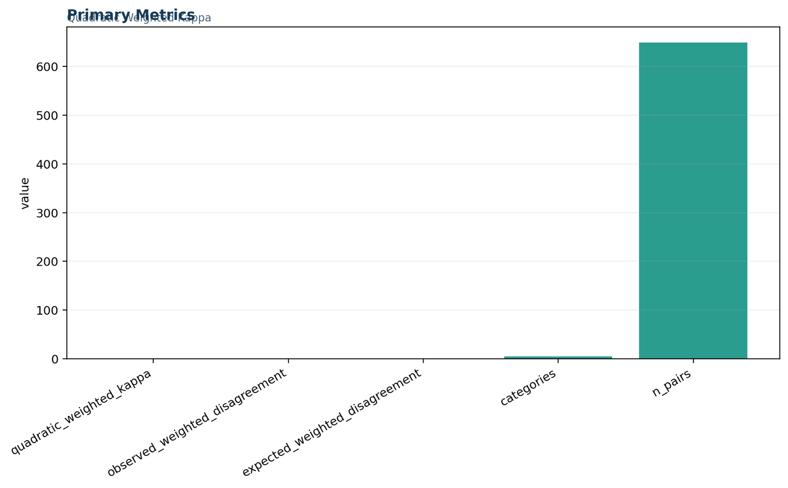
Python Figure 1: Primary metrics
The chart places quadratic weighted kappa, observed disagreement, expected disagreement, category count, and sample size on one axis. The 649-pair bar dominates visually, so the exact ledger must be read with the graphic: κw = 0.827339, Do = 0.034476, De = 0.199675, q = 5, and n = 649.
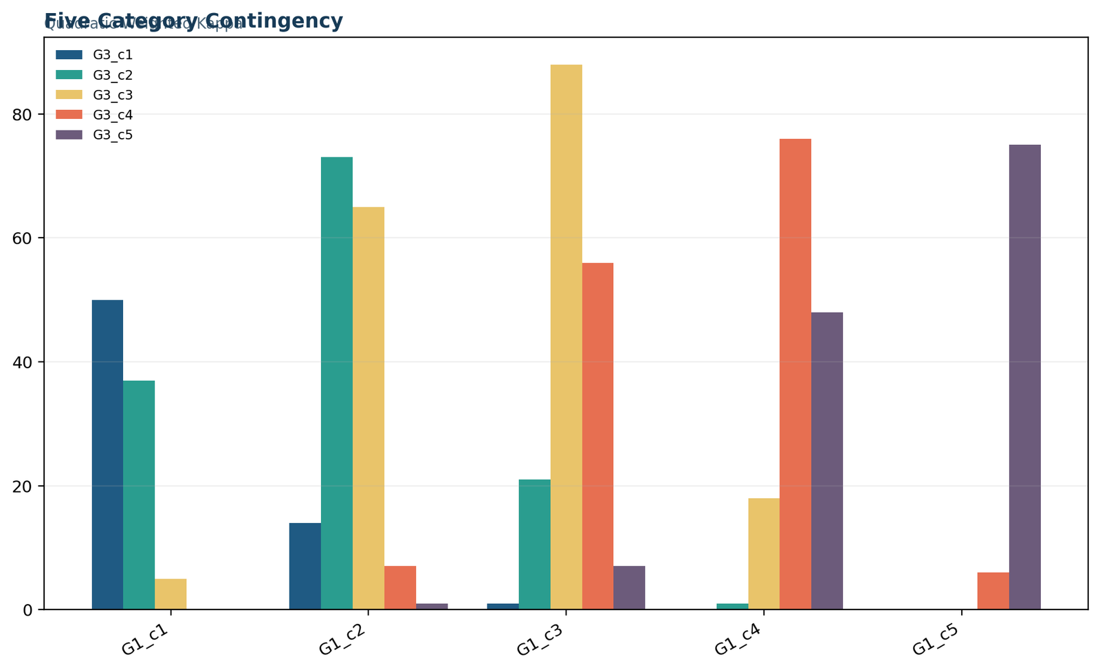
Python Figure 2: Five-category contingency
The grouped bars reproduce every row of the 5 x 5 table. Diagonal peaks occur at 50, 73, 88, 76, and 75. The largest off-diagonal bars are the upward adjacent transitions 2 to 3, 3 to 4, 4 to 5, and 1 to 2.
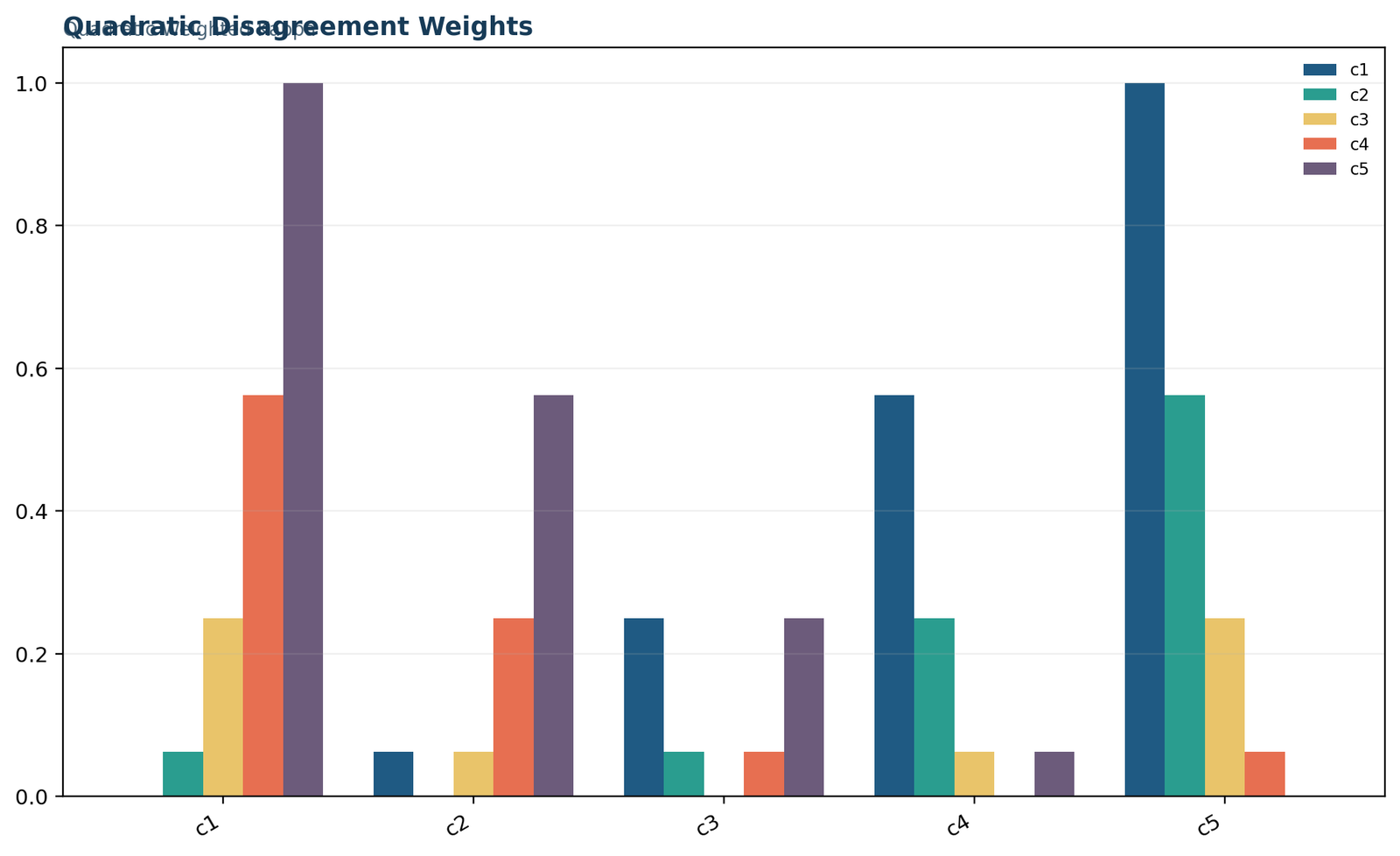
Python Figure 3: Quadratic disagreement weights
The weight profile is symmetric around the diagonal. Exact matches carry weight 0; one-, two-, three-, and four-step mismatches carry 0.0625, 0.25, 0.5625, and 1.00. This chart explains why nearby errors contribute little to observed disagreement.
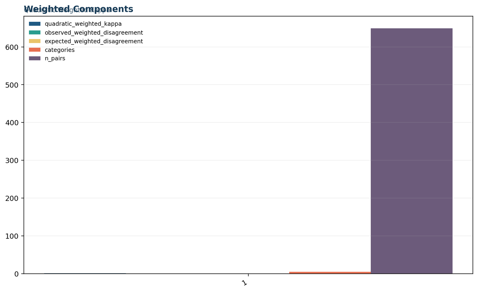
Python Figure 4: Weighted components
The component chart places the coefficient and disagreement terms beside q and n. The central comparison is not bar height against the sample-size bar but Do = 0.034476 versus De = 0.199675. Their ratio is 0.172661, leaving weighted kappa at 0.827339.
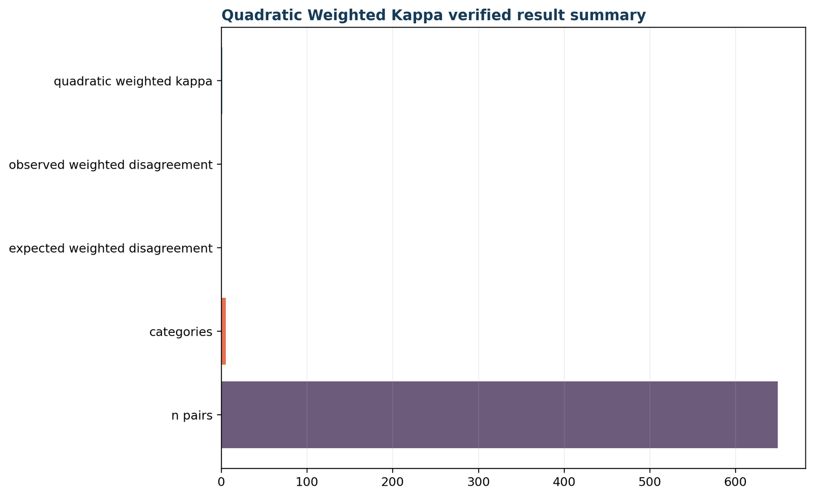
Python Figure 5: Verified result summary
The horizontal summary confirms the five reported fields. The long n-pairs bar and category bar are contextual counts; the three smaller analytic fields are the coefficient and disagreement terms. The values match the Excel workbook to numerical precision.
What the Python contingency figure adds
The coefficient alone cannot reveal whether disagreement is scattered, concentrated in one category, or directionally asymmetric. The grouped contingency chart shows a diagonal ridge and a stronger pattern above the diagonal. Category 5 is especially stable from G1 to G3: 75 of 81 G1 category-5 cases remain category 5, while six fall to category 4.
Category 2 shows a different pattern. Seventy-three cases remain category 2, but 65 move to category 3 and seven move to category 4. Weighted kappa treats the 65 adjacent movements gently but assigns a larger penalty to the seven two-step movements and the one three-step movement to category 5.
What the Python weight figure adds
The weight chart makes the loss function visible. It prevents the common error of reporting “quadratic” without defining what the term means. With five categories, an adjacent disagreement receives 0.0625 rather than the 0.25 used by linear weighting. A two-step disagreement receives 0.25 rather than 0.50.
The visual also confirms symmetry: moving from category 1 to 3 receives the same penalty as moving from 3 to 1. If a study needs different penalties for upward and downward errors, a custom asymmetric matrix should be specified and reported instead of using the standard quadratic scheme.
For broader Python workflows, review reliability analysis in Python, categorical data analysis in Python, correlation in Python, and descriptive statistics. Those guides complement the current ordinal agreement analysis but do not change the verified weighted kappa result.
Weighted kappa charts in R
The R workflow independently reproduces the same five-category visual and numerical result ledger.
The R figures use the same verified chart files and values so the visual comparison across software is direct. Reproducing weighted kappa independently is useful because packages may differ in how they label weight matrices, order factor levels, handle missing values, or report agreement rather than disagreement weights.
R Figure 1: Primary metrics
The R metric ledger confirms n = 649, q = 5, Do = 0.034476, De = 0.199675, and quadratic weighted kappa = 0.827339. These are the quantities that should be compared across R functions or a manual implementation.
R Figure 2: Five-category contingency
The R contingency view confirms 362 diagonal pairs and 287 mismatches. Bars immediately to the right of the diagonal dominate the errors, supporting strong near agreement and the observed shift toward higher G3 categories.
R Figure 3: Quadratic disagreement weights
The weight matrix uses squared normalized distances. An R function must receive factors in the intended 1-to-5 order; otherwise the displayed matrix and coefficient may no longer represent the substantive category distances.
R Figure 4: Weighted components
The observed disagreement is much smaller than expected disagreement. The component relationship, not the common y-axis scale, drives the coefficient: 1 – 0.034476/0.199675 = 0.827339.
R Figure 5: Verified result summary
The final R summary agrees with Python and Excel. The absence of cross-software differences supports correct category ordering, complete-case handling, and use of the quadratic disagreement formula.
R factor-level control
R may order character categories alphabetically unless levels are explicitly declared. Numeric labels 1 through 5 are naturally ordered here, but descriptive labels such as “low,” “middle,” and “high” can be reordered unintentionally. Analysts should create ordered factors with the same level list for both ratings and include all five levels even when a category is absent from one margin.
The contingency table should be inspected before any coefficient is accepted. Its row totals must be 92, 160, 173, 143, and 81; its column totals must be 65, 132, 176, 145, and 131; and its diagonal must be 50, 73, 88, 76, and 75.
R package output checks
Some functions report unweighted kappa by default, while others require a weight name such as “equal,” “squared,” or a custom vector. Package terminology is not universal. Inspect documentation and compare the returned value with the verified targets: .439485 unweighted, .664272 linear, and .827339 quadratic.
When a function displays an agreement-weight matrix, adjacent agreement weight should be .9375 under the quadratic scheme because it is 1 – .0625. A function displaying disagreement weights should show .0625. Both can be correct; mixing the displayed matrix with the wrong formula is not.
Related R resources include reliability analysis in R, categorical data analysis in R, correlation in R, and correlation matrix. Weighted kappa remains the correct primary measure here because the outcome is paired ordinal agreement rather than internal consistency or ordinary association.
How to analyze weighted kappa in SPSS
SPSS verifies the table and ordinary kappa, while the quadratic coefficient requires an explicit weighted calculation.
The SPSS output imports 649 rows, creates the five-category G1 and G3 variables, and runs a crosstabulation with counts, row percentages, column percentages, expected counts, and residuals. It also reports ordinary Cohen’s kappa, Spearman correlation, and the distribution of squared category distance. These outputs are important diagnostics for the primary weighted kappa calculation.
SPSS table result
The case-processing summary shows 649 valid pairs and zero missing. The crosstabulation matches the verified 5 x 5 matrix. SPSS reports ordinary kappa = .439, asymptotic standard error = .025, approximate test statistic = 22.038, and approximate significance p < .001.
That coefficient treats every off-diagonal mismatch equally. It is a useful comparison and confirms positive exact agreement beyond chance, but it is not the quadratic weighted kappa of .827339.
SPSS supporting diagnostics
The category scores have Spearman correlation .850, p < .001. The squared-distance variable has mean .0345, standard deviation .05404, minimum 0, and maximum .5625. Its frequencies are 362 at 0, 265 at .0625, 21 at .25, and one at .5625.
The mean of that squared-distance variable is the observed quadratic weighted disagreement Do. SPSS therefore verifies the observed component directly even though the standard crosstab kappa table remains unweighted.
| SPSS output | Verified value | Role in the analysis | Reporting caution |
|---|---|---|---|
| Valid cases | 649 | Confirms complete paired sample | Do not combine unpaired or duplicate rows. |
| Ordinary kappa | .439 | Exact-category chance-corrected comparison | Not the weighted coefficient. |
| Spearman correlation | .850 | Supporting ordinal association | Correlation is not agreement. |
| Mean squared distance | .0345 | Observed quadratic disagreement | Expected disagreement is still needed. |
| Distance frequencies | 362, 265, 21, 1 | Explains near versus distant errors | Retain exact decimals before rounding. |
A complete SPSS weighted calculation can be performed with an extension, embedded Python or R, MATRIX commands, or exported table components. Whatever route is used, the final result should reproduce De = 0.199675 and weighted kappa = 0.827339. The expected weighted disagreement is not the ordinary expected exact disagreement of 0.788951 or its complement; it must be calculated with the quadratic distance matrix.
For additional SPSS context, see reliability analysis in SPSS, categorical data analysis in SPSS, correlation in SPSS, and chi-square testing. The current analysis is paired agreement, so independent-sample interpretations of the crosstab are not the primary purpose.
How to calculate weighted kappa in Excel
The worked workbook exposes the row-level transformations, formula checks, diagnostics, and verified result ledger.
Excel is useful for learning the mechanics of weighted kappa because every component can be displayed in cells. The worked analysis contains Guide, Data_Input, Working, Calculations, Diagnostics, and Reporting sheets. The workbook retains 649 raw G1-G3 pairs, calculates the five-category transforms and row penalties, and compares the formula output with independently verified Python and R results.
1. Prepare the paired data
Place G1 and G3 in separate columns with one row per case. Check that the row count is 649 and that both columns refer to the same student. Preserve raw variables and perform recoding in formula-driven working columns rather than overwriting the source.
2. Create ordered classes
Map each grade to the documented category boundaries. The workbook creates category 1 for values through 8, category 2 for 9-10, category 3 for 11-12, category 4 for 13-14, and category 5 for 15 or higher.
3. Calculate row distance
For each pair, calculate squared distance and divide by 16. The mean of the 649 row penalties is Do = 0.0344761171. A frequency table should match 362 zeros, 265 values of .0625, 21 values of .25, and one value of .5625.
Observed table and expected table
Create the 5 x 5 observed table with COUNTIFS or a PivotTable. Calculate each expected count as row total times column total divided by 649. Convert both tables to proportions. Build the 5 x 5 quadratic disagreement matrix with (row category – column category)2/16.
Use SUMPRODUCT between the observed proportion table and weight matrix to obtain Do. Use SUMPRODUCT between the expected proportion table and the same weight matrix to obtain De. The verified values are 0.0344761171 and 0.1996751551.
Final formula and checks
The final cell calculates 1 – Do/De and returns 0.8273389742. The Calculations sheet records the category count, pair count, observed disagreement, expected disagreement, and exact result. The Reporting sheet compares workbook values with reference values and shows zero or machine-level differences.
Formula checks should also confirm that the observed table totals 649, row totals equal the G1 category counts, column totals equal the G3 counts, and the weight matrix is symmetric with zeros on the diagonal and ones in the opposite corners.
When learning how to calculate weighted Cohen kappa in Excel, the most common mistake is using the average row distance as the final coefficient. The average squared distance is Do, not weighted kappa. Chance correction requires De. Another common error is calculating expected counts from equal category probabilities rather than the observed margins.
The workbook’s exact result agrees with Python and R. This cross-software agreement is stronger evidence than rounded visual comparison because the difference is zero to displayed precision. The only tiny difference for observed disagreement is about 6.94 x 10⁻¹⁸, which is ordinary floating-point representation rather than a statistical discrepancy.
Readers working with broader spreadsheet analyses can review correlation in Excel, regression in Excel, confidence intervals, and effect size. Those methods use different formulas, but the same principles of transparent inputs, formula-driven calculations, and independent verification apply.
Weighted kappa compared with related agreement measures
Choose the statistic from the measurement scale, number of raters, pairing structure, and scientific question.
Weighted kappa is specifically designed for two paired ordinal ratings. It should not be used automatically for every reliability problem. The table below distinguishes common alternatives and shows why a familiar coefficient may answer a different question.
| Method | Typical scale/design | Primary question | Relationship to weighted kappa |
|---|---|---|---|
| Cohen’s kappa | Two paired nominal ratings | Exact agreement beyond chance | Use when categories are unordered or all mismatches are equally serious. |
| Weighted kappa | Two paired ordinal ratings | Distance-sensitive agreement beyond chance | Primary method for the current five-category design. |
| Fleiss kappa | Multiple raters, nominal categories | Multi-rater agreement beyond chance | Number of raters differs; standard form does not preserve ordinal distance. |
| Krippendorff’s alpha | Multiple raters, flexible scales, missing ratings | Reliability using a specified distance function | More general design; may incorporate ordinal distance. |
| Intraclass correlation coefficient | Continuous or near-continuous ratings | Consistency or absolute agreement | Retains numeric scale information; quadratic kappa can be related under restricted conditions but is not automatically an ICC. |
| Spearman correlation | Ordered or continuous paired values | Monotonic association | Does not require same categories or equal levels. |
| McNemar’s test | Paired binary categories | Marginal change or asymmetry | Tests change rather than agreement. |
| McNemar-Bowker test | Paired multicategory ratings | Symmetry of off-diagonal transitions | Complements weighted kappa when directional change matters. |
Weighted kappa versus ICC
Both can reward near agreement, and quadratic weighted kappa has mathematical connections to certain ICC formulations when categories are equally spaced and other conditions hold. However, the design statements are not interchangeable. ICC models distinguish random or fixed raters, consistency or absolute agreement, and single or average measurements. Weighted kappa requires an explicit category and weight definition.
Weighted kappa versus correlation
The worked Spearman correlation of .850 is close to the quadratic coefficient of .827, but similarity is accidental rather than definitional. Correlation remains high when one rating is consistently shifted upward. Weighted kappa responds to category separation and the chance structure of the margins. Reporting both can describe association and agreement without conflating them.
Weighted kappa versus scale reliability
Cronbach’s alpha, McDonald’s omega, Guttman’s lambda, and split-half reliability examine relationships among items or test halves. Weighted kappa examines paired category assignments to the same cases. A high internal-consistency coefficient does not imply high rater agreement.
Item diagnostics such as item-total correlation and corrected item-total correlation are also distinct. They identify how individual items align with a scale total, whereas weighted kappa evaluates two classifications. Binary-test reliability coefficients such as KR-20 and KR-21 do not replace agreement analysis.
Weighted kappa assumptions, diagnostics, and limitations
The coefficient is meaningful only when pairing, category order, weighting, and data quality are defensible.
Unlike a parametric mean comparison, weighted kappa does not require normally distributed ratings. Its important assumptions are structural: correct case pairing, independent pairs, identical ordered categories, prespecified weights, valid coding, and a cross-classification table that represents the target population and rating process.
| Diagnostic | Why it matters | Worked evidence | Corrective action |
|---|---|---|---|
| Pair alignment | A mismatched row compares different cases. | 649 paired G1-G3 rows. | Use stable IDs and verify joins before recoding. |
| Common category order | Weights depend on distance between corresponding levels. | Both variables use categories 1 through 5 with identical cut points. | Declare ordered levels explicitly in every program. |
| Independent cases | Standard uncertainty treats pairs as independent. | One pair per student. | Use clustered or multilevel methods for repeated nested pairs. |
| Prespecified weights | Post-hoc weight choice can inflate the preferred result. | Quadratic squared-distance penalties documented. | Justify weights from consequences or protocol. |
| Marginal distributions | Prevalence affects expected agreement. | G3 shifts toward category 5. | Report row and column totals with the coefficient. |
| Sparse cells | Empty or tiny cells can destabilize uncertainty. | Several distant cells are zero; only one three-step mismatch. | Use appropriate bootstrap checks and avoid overinterpreting rare transitions. |
| Missing data | Complete-case selection may change margins. | Zero missing in the analyzed variables. | State the missing-data rule and compare included cases. |
Prevalence and bias effects
Kappa coefficients use a chance benchmark derived from the margins. When one category dominates both ratings, raw agreement can be high while kappa is lower than expected by readers. When margins differ, expected agreement and directional patterns also change. This is not necessarily a flaw; it is part of the coefficient’s definition.
The current margins are not identical. G1 has 81 cases in category 5, whereas G3 has 131. The coefficient remains high because individual pairs are close, but the shift should be discussed. Consider reporting category prevalence, exact agreement, and a symmetry or marginal-homogeneity analysis.
Category number and spacing
Adding more categories generally creates more opportunities for near disagreement and may change the coefficient. Quadratic weights assume equal spacing between adjacent numeric category codes. If the practical difference from category 1 to 2 is not comparable with the difference from 4 to 5, standard weights may misrepresent loss.
Collapsing categories can raise exact agreement but may hide meaningful distinctions. Splitting categories can lower exact agreement while preserving strong weighted agreement. Category construction should be substantive, stable, and documented before analysis.
Inspecting the cross-table residuals is useful. Every diagonal count exceeds its independence expectation: 50 versus 9.21 in category 1, 73 versus 32.54 in category 2, 88 versus 46.92 in category 3, 76 versus 31.95 in category 4, and 75 versus 16.35 in category 5. Large positive diagonal residuals confirm that exact matches are concentrated far beyond chance. Several distant off-diagonal cells are zero or far below expectation.
Uncertainty can be affected when bootstrap samples omit a rare category. Analysts should keep the full factor-level set, define a reproducible handling rule, and report the number of valid replications. A narrow confidence interval does not eliminate design bias. Good reliability evidence begins with representative sampling, blinded rating, clear operational definitions, and stable category use.
General diagnostic concepts are discussed in outlier detection, sampling bias, sampling methods, and Type I and Type II error. Their details differ from weighted kappa, but they reinforce the need to connect statistical output with data-generation quality.
How to improve ordinal agreement and study design
Better agreement comes from clearer categories, controlled rating procedures, and feedback based on specific disagreement patterns.
A low or unstable weighted kappa should not be treated only as a number to increase. The purpose of reliability work is to identify preventable variation while preserving meaningful distinctions. Improvements should target the categories, instructions, rater training, case sampling, timing, and decision process that generated the table.
Clarify boundary cases
Most disagreements occur near category thresholds. Provide anchor examples just below and above every boundary, decision rules for incomplete evidence, and guidance for ties. In the worked table, the largest errors are adjacent upward transitions, so category boundaries deserve more attention than extreme-category confusion.
Use structured training
Raters should practice on representative cases, compare rationales, and receive feedback before the reliability sample begins. Training should not use the final test cases. Recalibration sessions can be scheduled when the task lasts long enough for drift to occur.
Blind prior information
When the same rater scores twice, conceal prior scores and randomize case order. When two raters score independently, prevent discussion until both ratings are recorded. Blinding reduces memory, consensus pressure, and anchoring.
Sample the full scale
A reliability sample dominated by easy middle cases may overstate performance for rare endpoints. Include sufficient cases from every category and enough boundary cases to evaluate the decisions that matter. Report how cases were selected.
Audit direction, not only distance
Symmetric weights treat upward and downward errors equally. If one direction is more costly, report directional counts and consider a justified asymmetric loss matrix. The current table has 226 upward and 61 downward transitions, so direction carries substantive information.
Separate reliability from validity
Agreement can improve through shared misunderstanding. Validate the rubric, reference standard, or category definitions separately. High weighted kappa supports reproducibility under the chosen rules; it does not prove that those rules classify the construct correctly.
For the current example, category 2 has the lowest exact row agreement at 45.6%, followed by category 3 at 50.9%. Category 5 has the highest exact row agreement at 92.6%. Improvement work should therefore focus on distinctions among categories 2, 3, and 4 rather than spending equal effort on every possible cell. The 65 transitions from 2 to 3 and 56 transitions from 3 to 4 are especially informative.
Reliability monitoring can include intra-rater reliability, inter-rater reliability, and test-retest reliability as separate components. A rater can be self-consistent but differ from peers, or multiple raters can agree at one time while the process drifts later. The study design should match the intended use of the ratings.
How to report weighted kappa in APA style
State the design, category coding, weighting rule, sample size, coefficient, and supporting agreement pattern.
An APA-style weighted kappa report should be reproducible without forcing readers to guess the scale or weight convention. At minimum, identify the two ratings, the five ordered categories, the quadratic disagreement rule, the number of valid pairs, the coefficient, exact agreement, and the most important distance or direction findings.
Concise result
This version is appropriate when the table, weights, and software details are available elsewhere in the report. Do not add a confidence interval unless it has actually been calculated for the weighted coefficient.
Expanded result
This version shows why the coefficient is high and makes the weight convention explicit.
Software comparison statement
Python, R, and Excel independently reproduced quadratic weighted kappa = 0.8273389742, observed weighted disagreement = 0.0344761171, and expected weighted disagreement = 0.1996751551. The SPSS crosstabulation reproduced the five-category counts and reported ordinary kappa = .439, SE = .025, p < .001, while the squared-distance variable verified the observed quadratic disagreement.
Interpretive discussion statement
The high quadratic coefficient reflects the concentration of mismatches near the diagonal rather than a high exact-match percentage alone. G3 exceeded G1 in 226 cases and was lower in 61, indicating a directional upward shift that should be interpreted separately from agreement. No case differed by all four category steps.
| Reporting element | Worked content | Why include it |
|---|---|---|
| Ratings | Five-category G1 and G3 | Defines the paired variables. |
| Category coding | 0-8, 9-10, 11-12, 13-14, 15+ | Makes ordinal boundaries reproducible. |
| Weight scheme | Quadratic disagreement, (i-j)2/16 | Defines the estimand. |
| Sample size | N = 649 | States the evidence base. |
| Coefficient | κw = .827339 | Primary chance-corrected result. |
| Raw agreement | 55.78% exact; 96.61% within one category | Shows the observed pattern. |
| Direction | 226 upward; 61 downward | Separates change from agreement. |
| Uncertainty | Not supplied for the quadratic coefficient | Prevents borrowing the ordinary-kappa SE. |
Use italic N for the sample size and an italic p for significance values. Kappa is commonly represented with the Greek letter κ, but writing “weighted kappa” in prose is also clear. Include enough decimals for reproducibility in tables and normally round to two or three decimals in narrative text. A result of .827 should not be described as 82.7% agreement.
The reporting logic follows broader principles used in null and alternative hypotheses, confidence intervals, p-values, and effect sizes: identify the estimand, show uncertainty when available, describe the observed data pattern, and connect the statistic to the scientific decision.
Weighted kappa downloads and related guides
Use the verified reports and worked workbook to reproduce the five-category analysis.
The four downloadable files provide the Python report, R report, SPSS output, and formula-driven Excel workbook for the same weighted kappa example. Each file should be interpreted according to its role: Python and R reproduce the quadratic coefficient, SPSS verifies the table and supporting outputs, and Excel exposes the calculation ledger.
R weighted kappa reportIndependent R reproduction of the ordered table and weighted coefficient.Open PDF
SPSS weighted kappa outputCrosstabulation, ordinary kappa, correlation, and squared-distance diagnostics.Open PDF
Worked Excel analysisRaw paired data, recoding, calculations, diagnostics, and verified result ledger.Open workbook
Related reliability and agreement guides
For additional categorical inference, see the likelihood-ratio chi-square, G-test, Fisher’s exact test, chi-square goodness-of-fit test, and chi-square test for homogeneity. Those methods address distributional questions rather than the weighted agreement estimand developed here.
Weighted kappa frequently asked questions
Direct answers to calculation, interpretation, software, and reporting questions.
What is weighted kappa?
Weighted kappa is a chance-corrected agreement coefficient for two paired ordinal ratings. It gives partial credit to near matches and larger penalties to distant disagreements according to a prespecified weight matrix.
When should weighted kappa be used?
Use it when the same cases receive two ratings on the same ordered categories and disagreement distance is meaningful. Use ordinary Cohen’s kappa for nominal categories and an ICC for continuous measurements when its design assumptions are appropriate.
What is quadratic weighted kappa?
Quadratic weighted kappa uses squared normalized category distance. With five categories, disagreement penalties are 0, .0625, .25, .5625, and 1 for distances zero through four. The worked result is 0.827339.
What is linear weighted kappa?
Linear weighted kappa increases disagreement penalty in equal increments. With five categories, the penalties are 0, .25, .50, .75, and 1. The worked linear result is 0.664272.
What is the difference between weighted and unweighted kappa?
Unweighted kappa gives every mismatch full penalty. Weighted kappa uses ordinal distance. In the worked table, ordinary kappa is 0.439485, while quadratic weighted kappa is 0.827339 because most disagreements are adjacent.
How do I calculate weighted kappa?
Create the observed table, calculate expected proportions from the margins, define the weight matrix, compute observed and expected weighted disagreement, and use 1 – Do/De. The worked values are Do = .034476 and De = .199675.
How do I interpret weighted kappa of 0.827?
It indicates strong ordinal agreement under the stated quadratic weights. In this example, exact agreement is 55.78% and 96.61% of pairs are identical or adjacent. The coefficient should be interpreted with those patterns and the category margins.
Is weighted kappa a percentage?
No. A value of .827 is not 82.7% exact agreement. It means observed weighted disagreement is about 82.7% lower than expected weighted disagreement after the coefficient’s normalization.
Why is quadratic weighted kappa higher than linear weighted kappa?
Quadratic weights give more partial credit to adjacent mismatches. The data contain 265 adjacent disagreements, 21 two-step disagreements, one three-step disagreement, and no four-step disagreements, so quadratic weighting raises the coefficient substantially.
How do I choose weights for weighted kappa?
Choose weights from the practical loss associated with each category distance before examining results. Use linear weights for proportional loss, quadratic weights for squared-distance loss, or a justified custom matrix when standard spacing is inappropriate.
Can SPSS calculate weighted kappa?
The standard SPSS CROSSTABS kappa output shown here is ordinary kappa, not the quadratic coefficient. SPSS can support a weighted calculation through extensions, embedded code, MATRIX procedures, or exported table components. Verify the result against 0.827339.
What does the SPSS kappa value of .439 mean?
It is the ordinary chance-corrected exact agreement coefficient for the five-category table. SPSS reports SE = .025 and p < .001. It should be labeled unweighted kappa and not substituted for the primary quadratic result.
Can weighted kappa be calculated in Python and R?
Yes. Both languages can calculate it with validated packages or a direct matrix formula. Always control category order, missing values, and the weight convention. The Python and R reports reproduce 0.8273389742.
How do I calculate weighted kappa in Excel?
Build the observed and expected 5 x 5 proportion tables, create the quadratic weight matrix, use SUMPRODUCT for Do and De, and calculate 1 – Do/De. The worked workbook includes every step.
Does weighted kappa require normality?
No. It is based on category counts, not a normal distribution. Important requirements are correct pairing, independent cases, identical ordered categories, defensible weights, and valid handling of missing values.
Can weighted kappa be high when ratings change systematically?
Yes. Agreement can remain high when most changes are small and directional. In this example, 226 cases move upward and 61 downward, yet most disagreements are adjacent, so quadratic weighted kappa is .827.
Should I report exact agreement with weighted kappa?
Yes. Report exact agreement, near-agreement distances, margins, and direction when relevant. The worked example has 55.78% exact agreement and 96.61% within-one-category agreement.
What should be included in a weighted kappa report?
Include the two ratings, category definitions and order, weight scheme and convention, number of valid pairs, coefficient, uncertainty when available, raw exact agreement, distance distribution, marginal pattern, software, and any directional finding.