
Pearson Correlation, Spearman Correlation, SPSS Output Tables and APA Reporting
Correlation in SPSS: Pearson, Spearman, Output Interpretation and APA Reporting Guide
Correlation in SPSS is used when you want to test whether two variables move together, how strong that relationship is, and whether the relationship is statistically significant. This guide shows how to run a correlation test in SPSS, how to calculate Pearson correlation in SPSS, how to compute Spearman rank correlation in SPSS, how to read Sig. (2-tailed), how to interpret SPSS output pages, and how to write the result in APA style.
Quick Answer: Correlation in SPSS Result
The main SPSS correlation example focuses on the student performance variables G1, G2, and G3. These are grade-related numeric variables, so the strongest and clearest SPSS result is the academic-performance cluster. The strongest Pearson correlation is between G2 and G3, with approximately r = .919. The relationship between G1 and G2 is also very strong at approximately r = .865, and the relationship between G1 and G3 is very strong at approximately r = .826. With N = 649, these grade correlations are statistically significant at p < .001.
The practical interpretation is simple: students who score higher on earlier grade measures also tend to score higher on final grade performance. The strongest link is G2 with G3, which means the second-period grade is the closest grade-based companion of the final grade. This does not prove causation, but it gives strong evidence that the grade variables are closely aligned in the dataset.
Final interpretation: The SPSS output supports a very strong positive correlation among the grade variables. The strongest result is G2 with G3, so the final grade rises closely with the previous grade measure.
Important warning: Correlation in SPSS measures association, not causation. A large Pearson r does not prove that one grade causes the other; it shows that the two variables move together strongly.
Table of Contents
- What Is Correlation in SPSS?
- Pearson, Spearman and Kendall Correlation in SPSS
- Correlation Formula
- Null and Alternative Hypotheses
- Dataset and Variables Used
- How to Run Correlation in SPSS
- SPSS Output Interpretation
- SPSS Output Image-by-Image Explanation
- Assumptions for Pearson Correlation in SPSS
- SPSS Syntax for Correlation
- APA Reporting Wording
- Common Mistakes
- Downloads and Resources
- Related Guides
- FAQs
What Is Correlation in SPSS?
Correlation in SPSS is a statistical procedure that measures the direction and strength of association between two variables. The result is a correlation coefficient, usually written as r for Pearson correlation or ρ for Spearman correlation. The coefficient ranges from -1 to +1. Positive values mean the variables tend to increase together. Negative values mean one variable tends to increase when the other decreases. Values near zero mean little or no relationship.
In SPSS, the most common path is Analyze → Correlate → Bivariate. You select the variables, choose Pearson, Spearman, or Kendall, tick the correct significance option, and run the output. The Viewer then gives a table containing the correlation coefficient, the significance value, and the valid sample size for each pair.
This topic connects naturally with descriptive statistics, p-value, effect size, confidence interval, scatterplot interpretation, Q-Q plot normality check, and parametric vs nonparametric tests.
Simple definition: A correlation test in SPSS tells you whether two variables are related, whether the relationship is positive or negative, how strong it is, and whether it is statistically significant.
Pearson, Spearman and Kendall Correlation in SPSS
SPSS gives more than one correlation option. The best choice depends on the type of variables, shape of the relationship, and whether the data satisfy Pearson correlation assumptions.
| SPSS Correlation Type | Use It When | Example | Output Label |
|---|---|---|---|
| Pearson correlation | Both variables are numeric and the relationship is approximately linear. | G2 with G3 grade scores. | Pearson Correlation |
| Spearman correlation | Variables are ordinal, non-normal, or monotonic but not clearly linear. | Ranked studytime with final grade. | Correlation Coefficient under Spearman’s rho |
| Kendall’s tau-b | Ordinal variables, smaller samples, or many tied ranks. | Likert-style agreement scales. | Kendall’s tau-b |
| Partial correlation | You want the relationship between two variables while controlling another variable. | G2 and G3 while controlling absences. | Partial Correlations |
For the main grade example, Pearson is the primary method because G1, G2, and G3 are numeric grade variables. Spearman is still useful as a robustness check because it asks whether the rank ordering of students is similarly related across variables.
Correlation Formula
The Pearson correlation coefficient is based on standardized co-movement between two variables:
SPSS calculates this automatically, but the formula explains why outliers, nonlinearity, and restriction of range can affect the result. Pearson correlation is large when high values of one variable consistently match high values of the other variable and low values match low values.
Spearman correlation applies the same logic to ranks rather than raw values. That makes it useful when variables are ordinal or when a monotonic pattern is present but the raw-scale relationship is not perfectly linear.
Null and Alternative Hypotheses for Correlation in SPSS
| Hypothesis | Statement | Meaning |
|---|---|---|
| Null hypothesis | H0: ρ = 0 | There is no linear association between the two variables in the population. |
| Alternative hypothesis | H1: ρ ≠ 0 | There is a statistically detectable association between the variables. |
| Decision rule | p < .05 | Reject the null hypothesis at the 5% level. |
Decision for the grade example: Because the G1, G2, and G3 correlations are significant at p < .001, the null hypothesis of no association is rejected for those grade pairs.
Dataset and Variables Used
The example uses the student performance dataset, with G1, G2, and G3 as the main grade variables. These variables are well suited for showing how to read SPSS correlation output because the relationships are strong, positive, and easy to explain.
| Variable | Role | Why It Matters |
|---|---|---|
| G1 | First grade measure | Earlier academic performance indicator. |
| G2 | Second grade measure | Closest companion to final grade in the main result. |
| G3 | Final grade measure | Main outcome variable for interpretation. |
| studytime | Ordered study behavior variable | Useful for Spearman and supporting correlation examples. |
| failures | Prior failure count | Often negatively related to final performance. |
| absences | Attendance-related numeric variable | Useful for checking weak or inconsistent relationships. |
How to Run Correlation in SPSS
- Open the dataset in SPSS.
- Go to Analyze → Correlate → Bivariate.
- Move the variables into the Variables box, such as G1, G2, and G3.
- Select Pearson for numeric linear relationships.
- Select Spearman if you need a rank-based correlation.
- Choose Two-tailed unless you have a strong pre-registered one-direction hypothesis.
- Tick Flag significant correlations if you want SPSS to mark significant cells.
- Click OK and read the output table.
SPSS menu shortcut: Analyze → Correlate → Bivariate is the standard path for Pearson and Spearman correlation in SPSS.
SPSS Output Interpretation
The SPSS correlation table usually has three important lines for each pair: Pearson Correlation, Sig. (2-tailed), and N. Pearson Correlation is the coefficient. Sig. (2-tailed) is the p-value. N is the number of valid paired observations used for that correlation.
| Variable Pair | Pearson r | Sig. (2-tailed) | Interpretation |
|---|---|---|---|
| G2 with G3 | .919 | p < .001 | Very strong positive association. |
| G1 with G2 | .865 | p < .001 | Very strong positive association. |
| G1 with G3 | .826 | p < .001 | Very strong positive association. |
| Failures with G3 | About -.393 | p < .001 | Moderate negative relationship in the broader matrix context. |
The strongest relationship is G2 with G3. In practical terms, this means that students with higher G2 scores tend to have higher final G3 scores. Because the coefficient is close to 1, the relationship is very strong. The p-value is below .001, so the relationship is statistically significant.
The grade variables should not be interpreted as independent pieces of information. They form a strong academic-performance cluster. In later regression or prediction work, this cluster can create overlap or redundancy, so the analyst should also consider multicollinearity checks and variance inflation factor.
SPSS Output Image-by-Image Explanation
The following JPG images were exported from the SPSS output PDF. They are included so readers can compare the article interpretation with actual SPSS Viewer pages. The most important reading habit is consistent across the pages: identify the variable pair, read the coefficient, check Sig. (2-tailed), confirm N, and then inspect the supporting graph if one is shown.
SPSS Output Image 1: Page 0005
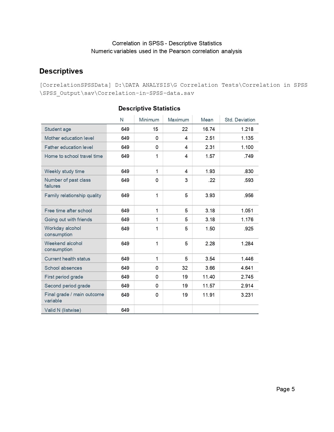
This early SPSS output image belongs to the setup and first-output part of the analysis. Use it to show readers that the data file was opened, the correlation procedure was executed, and the SPSS Viewer is producing formal output rather than a manual calculation. In a student report, this type of page is useful because it confirms the software context before the reader moves to coefficients, significance values, and graphs.
SPSS Output Image 2: Page 0007
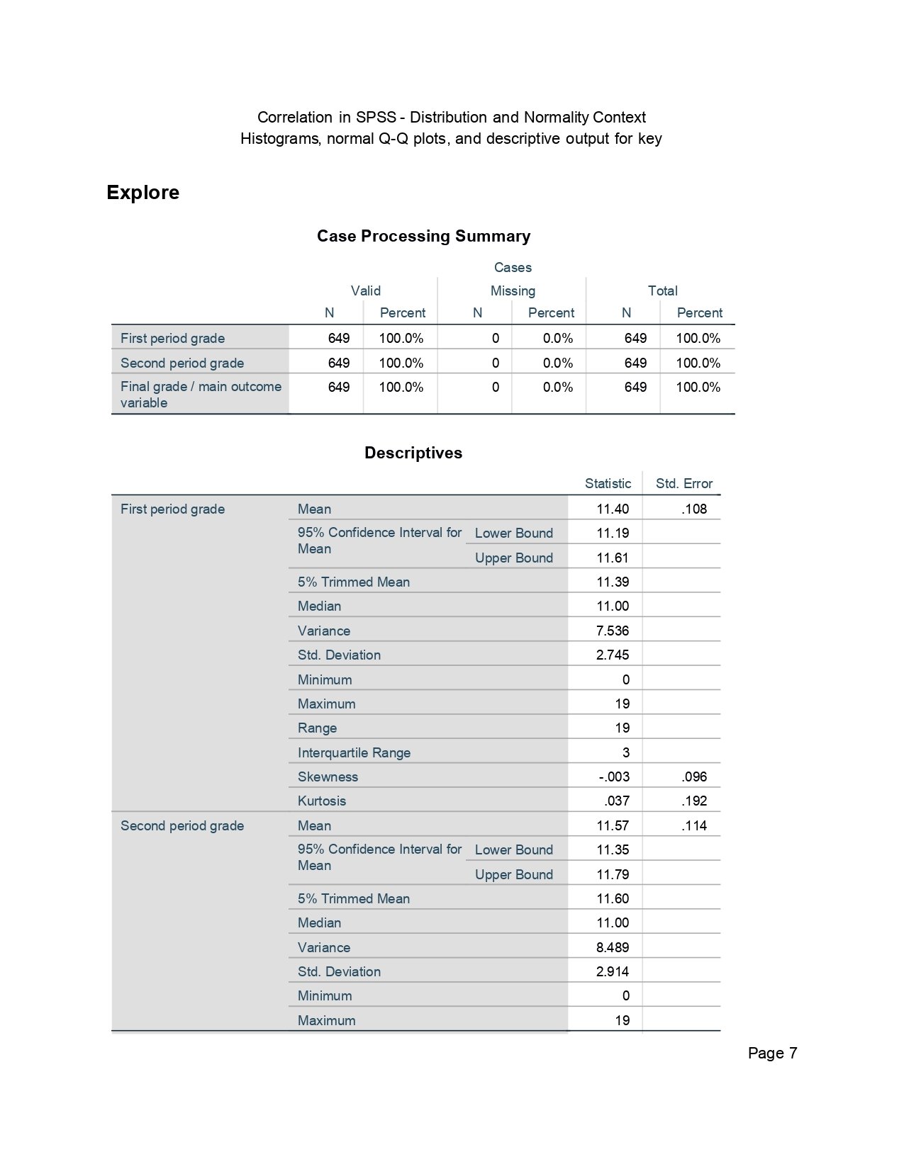
This early SPSS output image belongs to the setup and first-output part of the analysis. Use it to show readers that the data file was opened, the correlation procedure was executed, and the SPSS Viewer is producing formal output rather than a manual calculation. In a student report, this type of page is useful because it confirms the software context before the reader moves to coefficients, significance values, and graphs.
SPSS Output Image 3: Page 0008
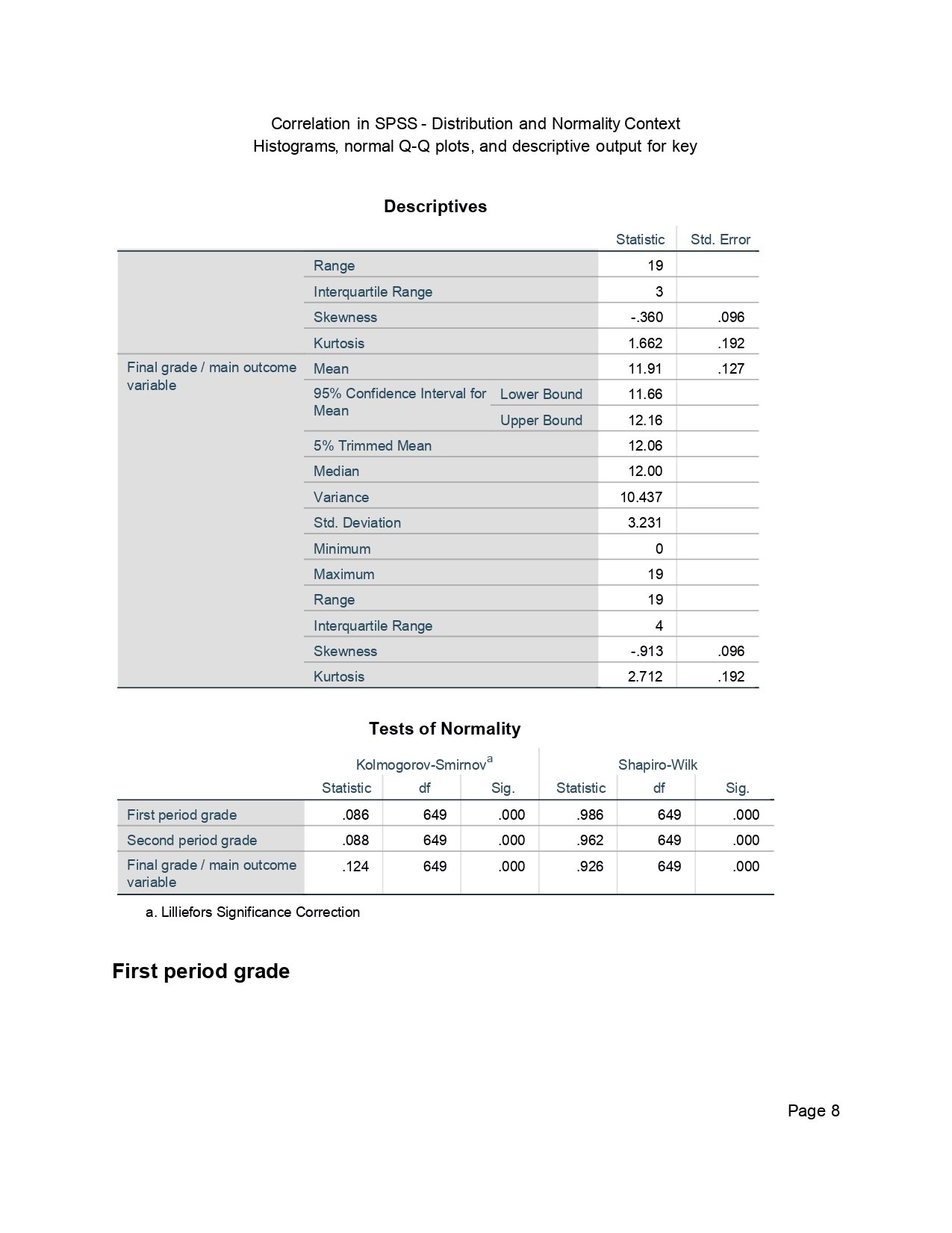
This SPSS output page supports the descriptive and matrix-reading part of the correlation workflow. For the student performance example, the main variables are G1, G2, and G3, with 649 valid cases. When reading this page, the important items are the variable names, valid N, mean or standard deviation information if present, and the Pearson or Spearman coefficient cells that connect grade variables together.
SPSS Output Image 4: Page 0009
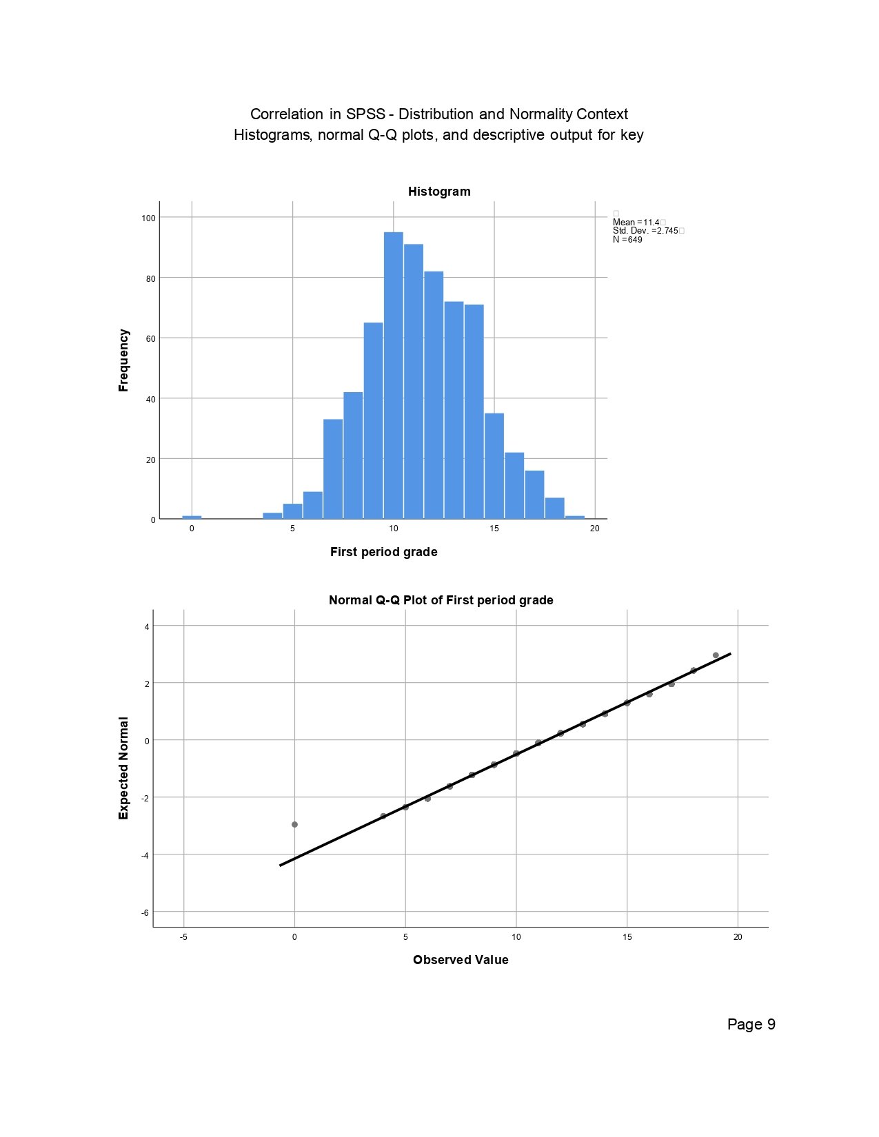
This SPSS output page supports the descriptive and matrix-reading part of the correlation workflow. For the student performance example, the main variables are G1, G2, and G3, with 649 valid cases. When reading this page, the important items are the variable names, valid N, mean or standard deviation information if present, and the Pearson or Spearman coefficient cells that connect grade variables together.
SPSS Output Image 5: Page 0010
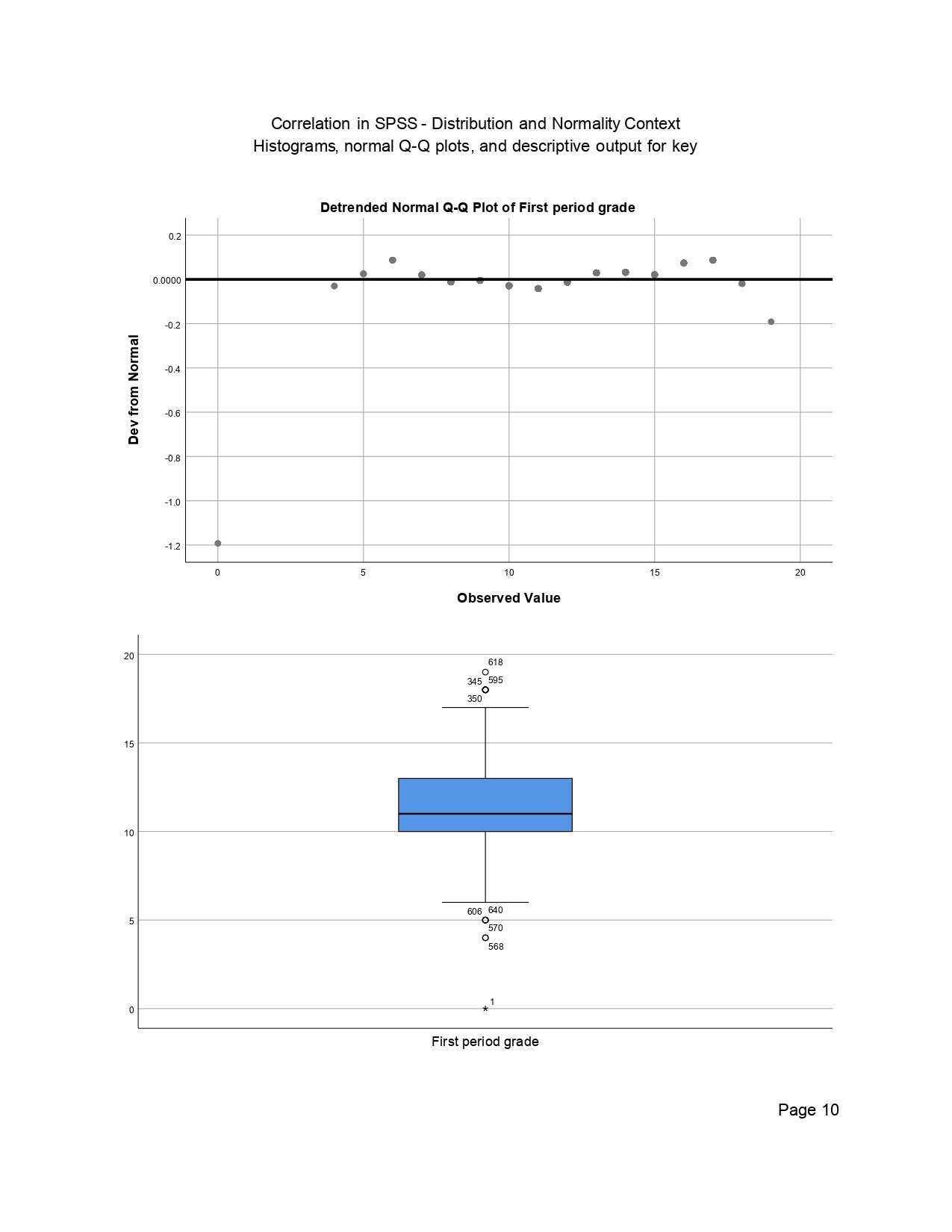
This SPSS output page supports the descriptive and matrix-reading part of the correlation workflow. For the student performance example, the main variables are G1, G2, and G3, with 649 valid cases. When reading this page, the important items are the variable names, valid N, mean or standard deviation information if present, and the Pearson or Spearman coefficient cells that connect grade variables together.
SPSS Output Image 6: Page 0011
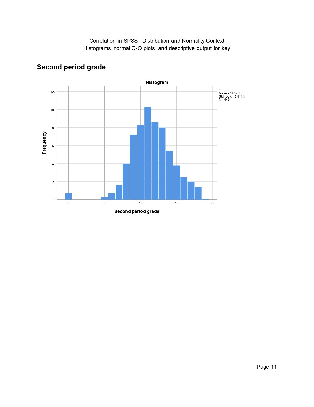
This SPSS output page supports the descriptive and matrix-reading part of the correlation workflow. For the student performance example, the main variables are G1, G2, and G3, with 649 valid cases. When reading this page, the important items are the variable names, valid N, mean or standard deviation information if present, and the Pearson or Spearman coefficient cells that connect grade variables together.
SPSS Output Image 7: Page 0012
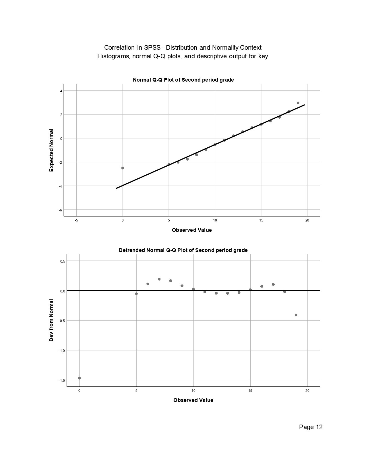
This SPSS output page supports the descriptive and matrix-reading part of the correlation workflow. For the student performance example, the main variables are G1, G2, and G3, with 649 valid cases. When reading this page, the important items are the variable names, valid N, mean or standard deviation information if present, and the Pearson or Spearman coefficient cells that connect grade variables together.
SPSS Output Image 8: Page 0013
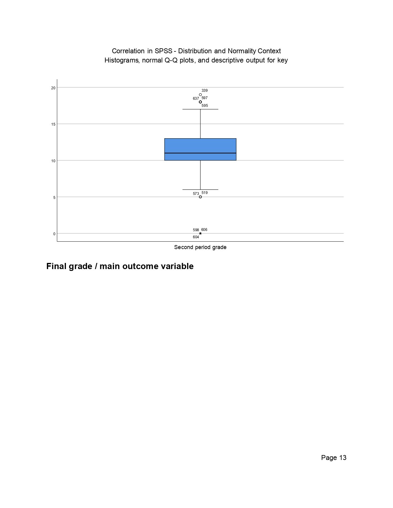
This SPSS output page supports the descriptive and matrix-reading part of the correlation workflow. For the student performance example, the main variables are G1, G2, and G3, with 649 valid cases. When reading this page, the important items are the variable names, valid N, mean or standard deviation information if present, and the Pearson or Spearman coefficient cells that connect grade variables together.
SPSS Output Image 9: Page 0014
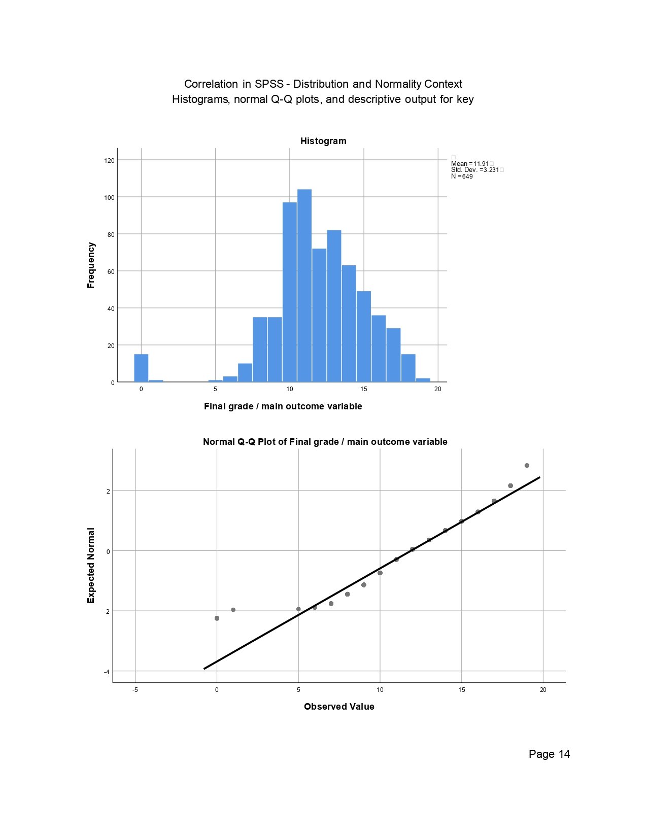
This output page helps readers move from raw SPSS tables into interpretation. In the main correlation result, G2 and G3 show the strongest positive relationship, followed by G1 with G2 and G1 with G3. The page should be interpreted by reading the coefficient first, then the Sig. (2-tailed) value, and finally the N value so that the statistical decision is not based on color or layout alone.
SPSS Output Image 10: Page 0015
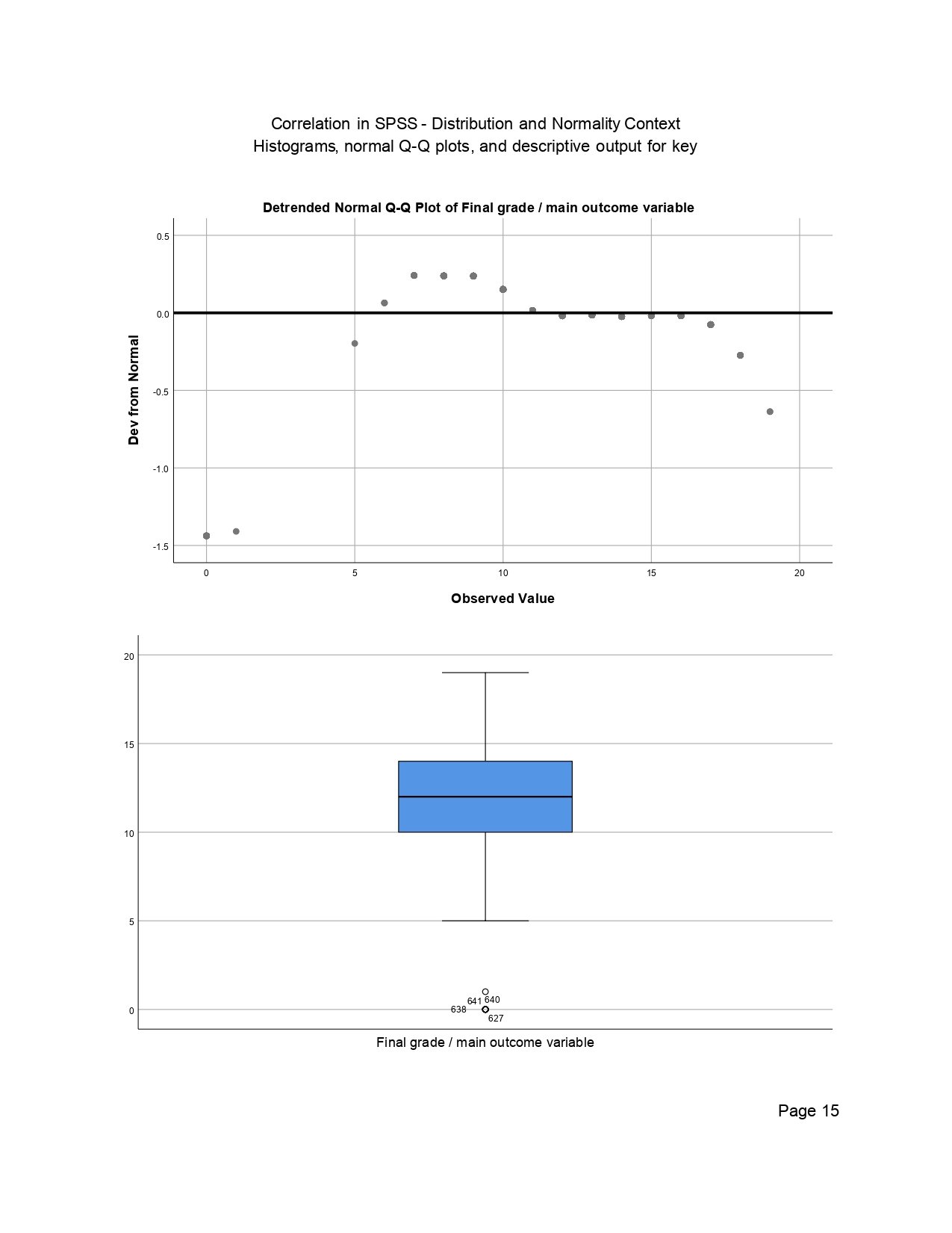
This output page helps readers move from raw SPSS tables into interpretation. In the main correlation result, G2 and G3 show the strongest positive relationship, followed by G1 with G2 and G1 with G3. The page should be interpreted by reading the coefficient first, then the Sig. (2-tailed) value, and finally the N value so that the statistical decision is not based on color or layout alone.
SPSS Output Image 11: Page 0017
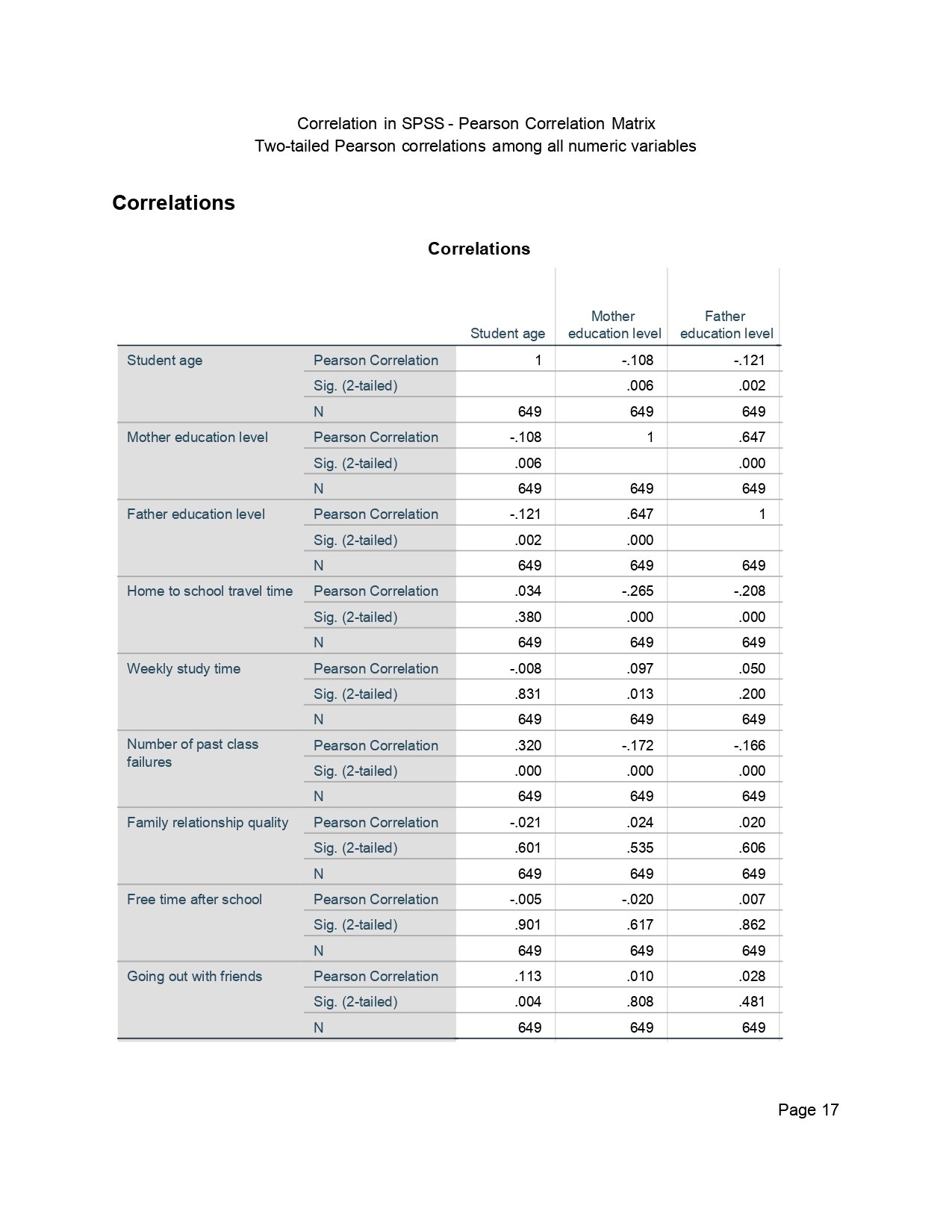
This SPSS image belongs to the visual-check section of the output. Correlation should not be interpreted from the coefficient table alone; scatterplots and supporting charts help confirm whether the relationship is broadly linear, whether extreme points are present, and whether the Pearson coefficient is a suitable summary. For G1, G2, and G3, the expected visual pattern is an upward cloud: higher earlier grades are associated with higher final grades.
SPSS Output Image 12: Page 0018
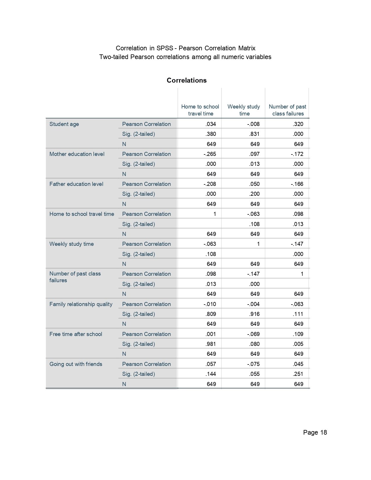
This SPSS image belongs to the visual-check section of the output. Correlation should not be interpreted from the coefficient table alone; scatterplots and supporting charts help confirm whether the relationship is broadly linear, whether extreme points are present, and whether the Pearson coefficient is a suitable summary. For G1, G2, and G3, the expected visual pattern is an upward cloud: higher earlier grades are associated with higher final grades.
SPSS Output Image 13: Page 0019
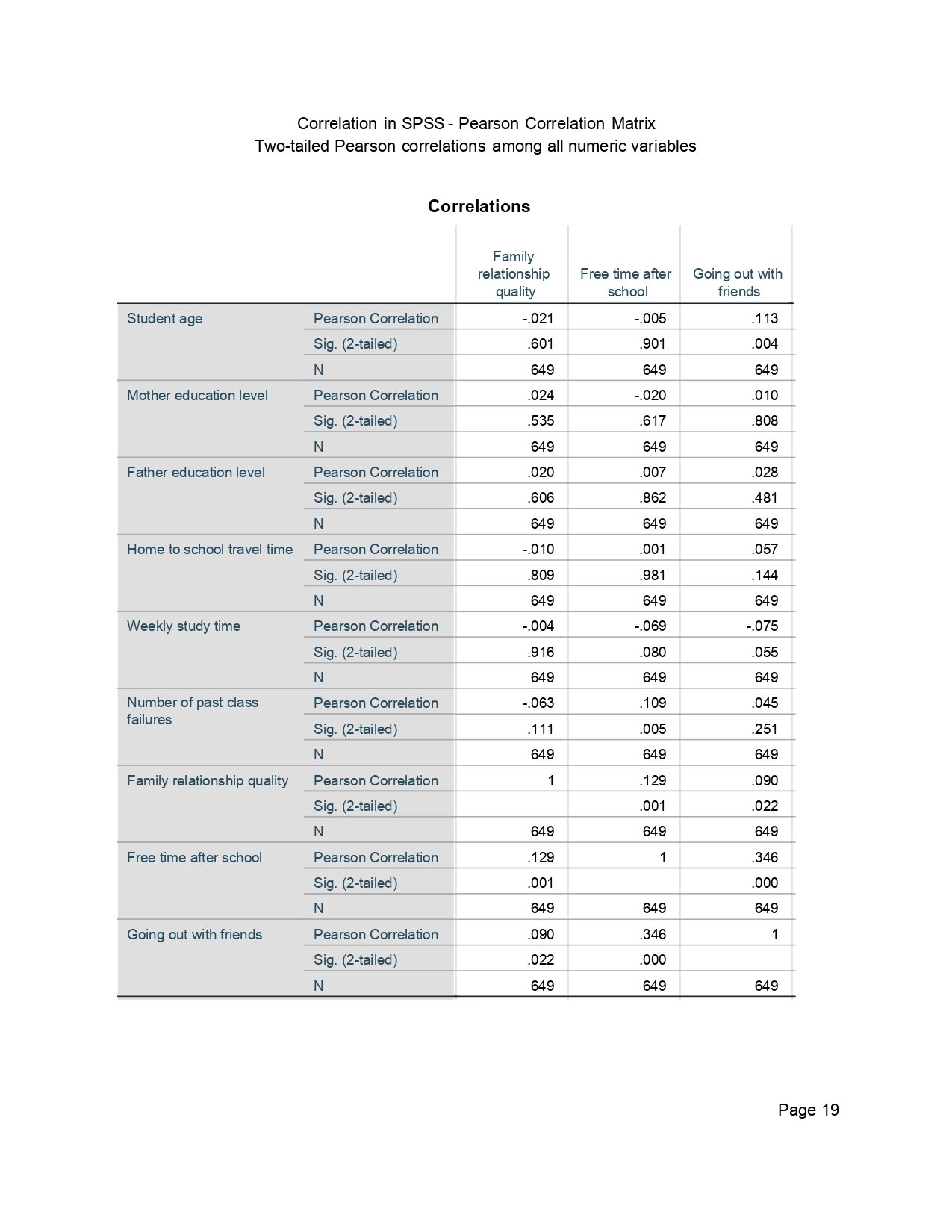
This SPSS image belongs to the visual-check section of the output. Correlation should not be interpreted from the coefficient table alone; scatterplots and supporting charts help confirm whether the relationship is broadly linear, whether extreme points are present, and whether the Pearson coefficient is a suitable summary. For G1, G2, and G3, the expected visual pattern is an upward cloud: higher earlier grades are associated with higher final grades.
SPSS Output Image 14: Page 0020
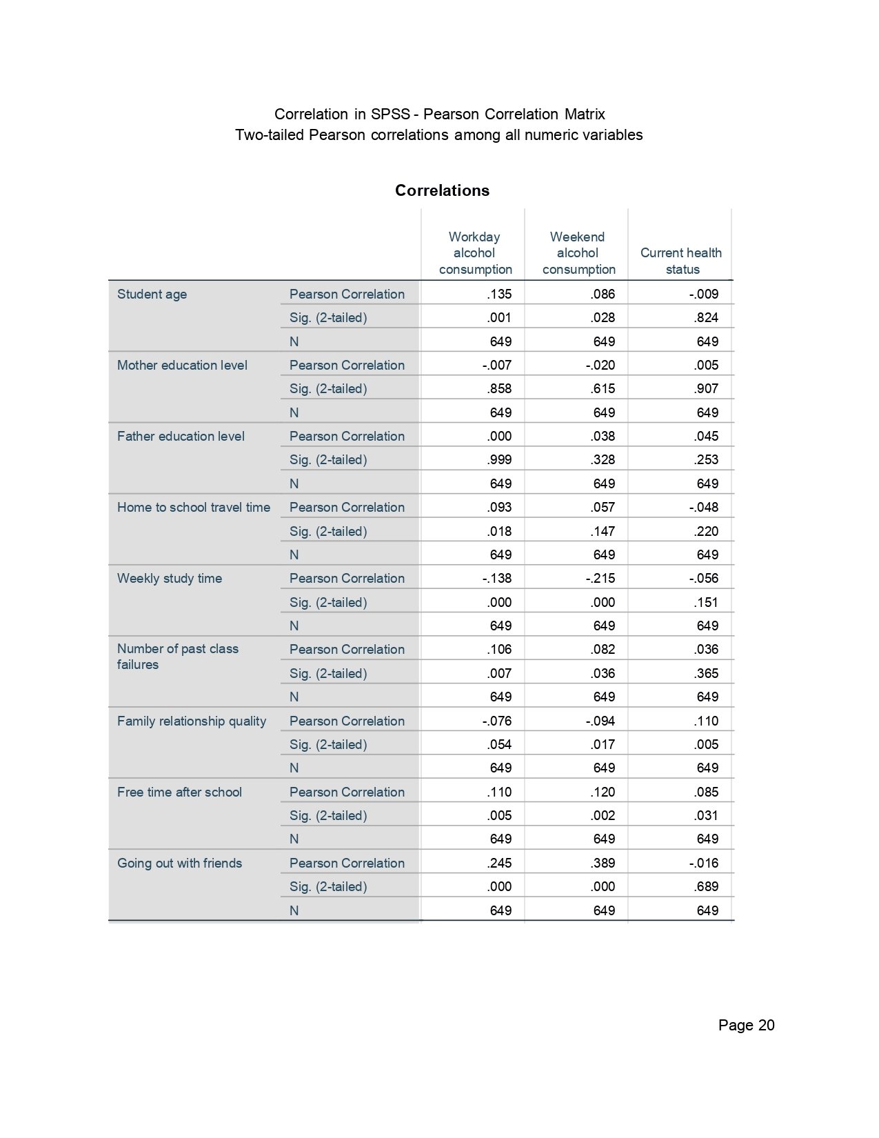
This SPSS image belongs to the visual-check section of the output. Correlation should not be interpreted from the coefficient table alone; scatterplots and supporting charts help confirm whether the relationship is broadly linear, whether extreme points are present, and whether the Pearson coefficient is a suitable summary. For G1, G2, and G3, the expected visual pattern is an upward cloud: higher earlier grades are associated with higher final grades.
SPSS Output Image 15: Page 0021
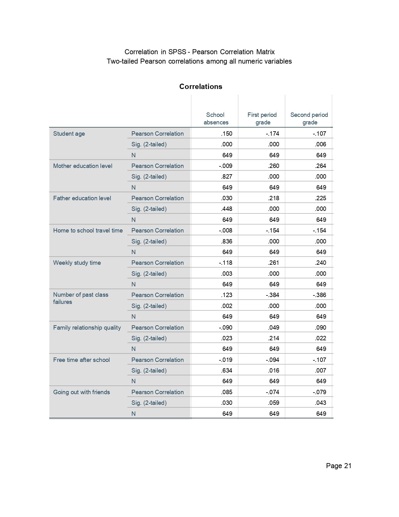
This SPSS image belongs to the visual-check section of the output. Correlation should not be interpreted from the coefficient table alone; scatterplots and supporting charts help confirm whether the relationship is broadly linear, whether extreme points are present, and whether the Pearson coefficient is a suitable summary. For G1, G2, and G3, the expected visual pattern is an upward cloud: higher earlier grades are associated with higher final grades.
SPSS Output Image 16: Page 0022
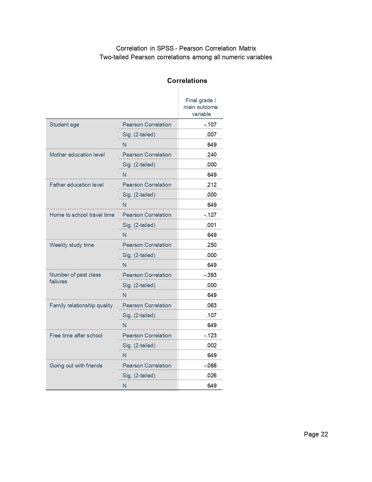
This SPSS image belongs to the visual-check section of the output. Correlation should not be interpreted from the coefficient table alone; scatterplots and supporting charts help confirm whether the relationship is broadly linear, whether extreme points are present, and whether the Pearson coefficient is a suitable summary. For G1, G2, and G3, the expected visual pattern is an upward cloud: higher earlier grades are associated with higher final grades.
SPSS Output Image 17: Page 0023
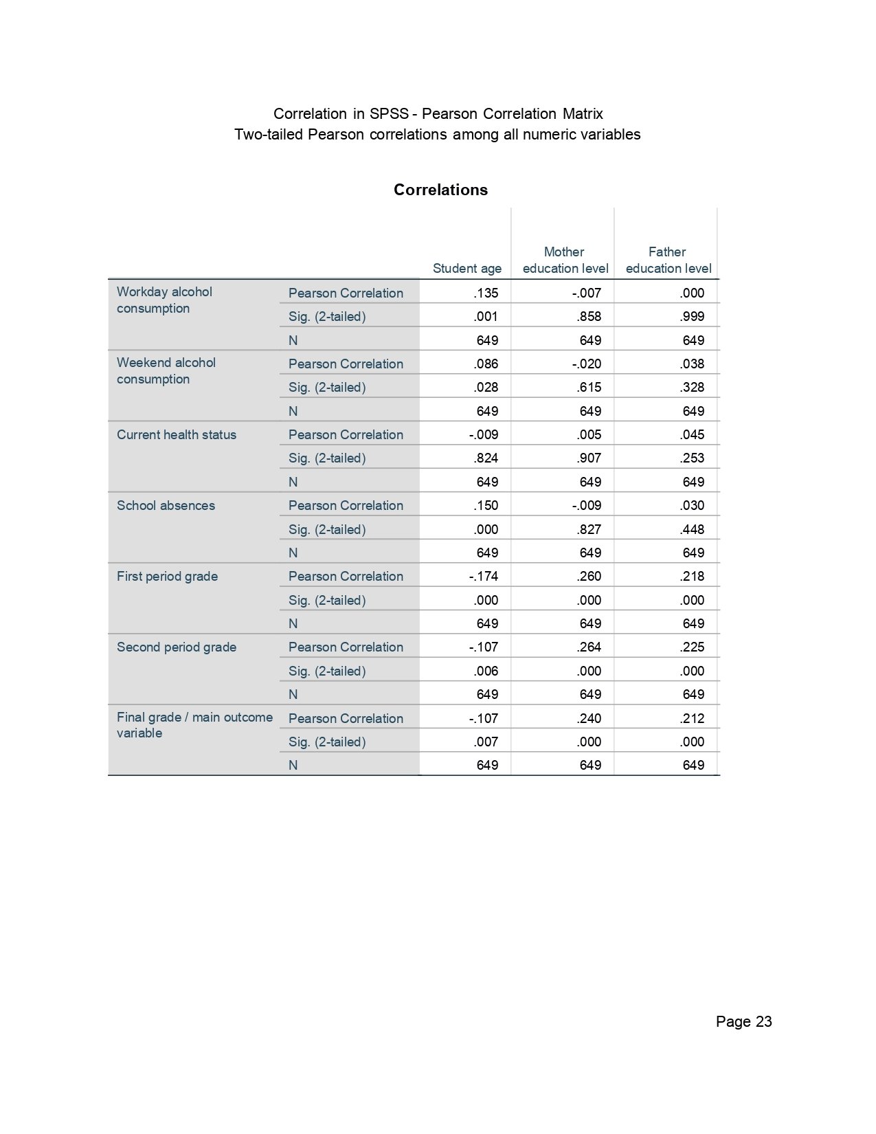
This SPSS image belongs to the visual-check section of the output. Correlation should not be interpreted from the coefficient table alone; scatterplots and supporting charts help confirm whether the relationship is broadly linear, whether extreme points are present, and whether the Pearson coefficient is a suitable summary. For G1, G2, and G3, the expected visual pattern is an upward cloud: higher earlier grades are associated with higher final grades.
SPSS Output Image 18: Page 0024
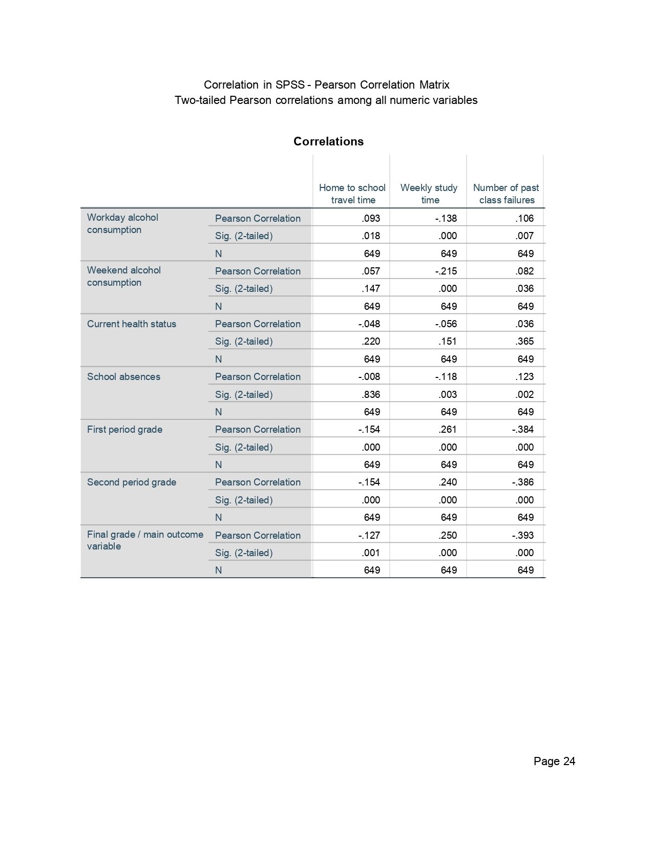
This SPSS image belongs to the visual-check section of the output. Correlation should not be interpreted from the coefficient table alone; scatterplots and supporting charts help confirm whether the relationship is broadly linear, whether extreme points are present, and whether the Pearson coefficient is a suitable summary. For G1, G2, and G3, the expected visual pattern is an upward cloud: higher earlier grades are associated with higher final grades.
SPSS Output Image 19: Page 0025
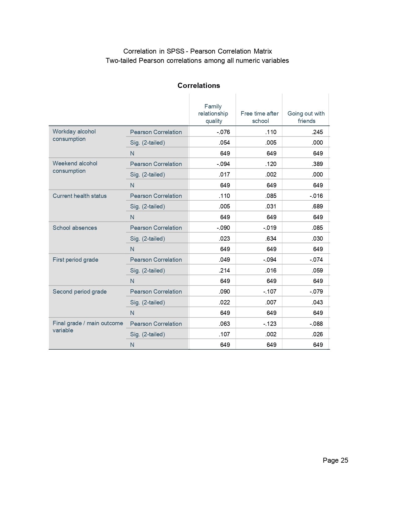
This page supports the diagnostic and reporting section of the SPSS output. A good correlation report should connect the visual pattern with the numeric matrix: the grades form a strong positive academic-performance cluster, while weaker background and behavior variables should not be overstated. Use this image to remind readers that a statistically significant correlation still needs a practical interpretation.
SPSS Output Image 20: Page 0026
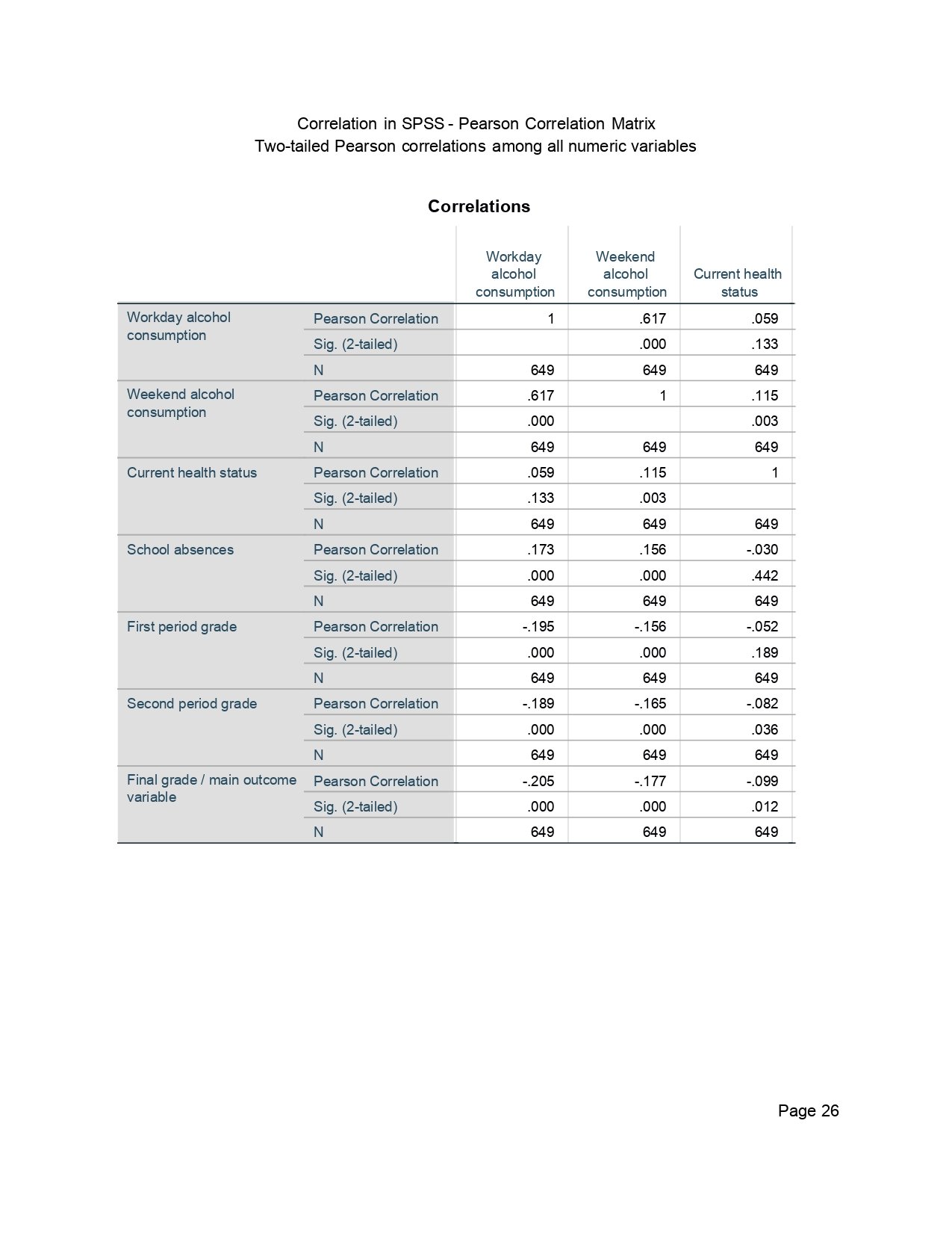
This page supports the diagnostic and reporting section of the SPSS output. A good correlation report should connect the visual pattern with the numeric matrix: the grades form a strong positive academic-performance cluster, while weaker background and behavior variables should not be overstated. Use this image to remind readers that a statistically significant correlation still needs a practical interpretation.
SPSS Output Image 21: Page 0027
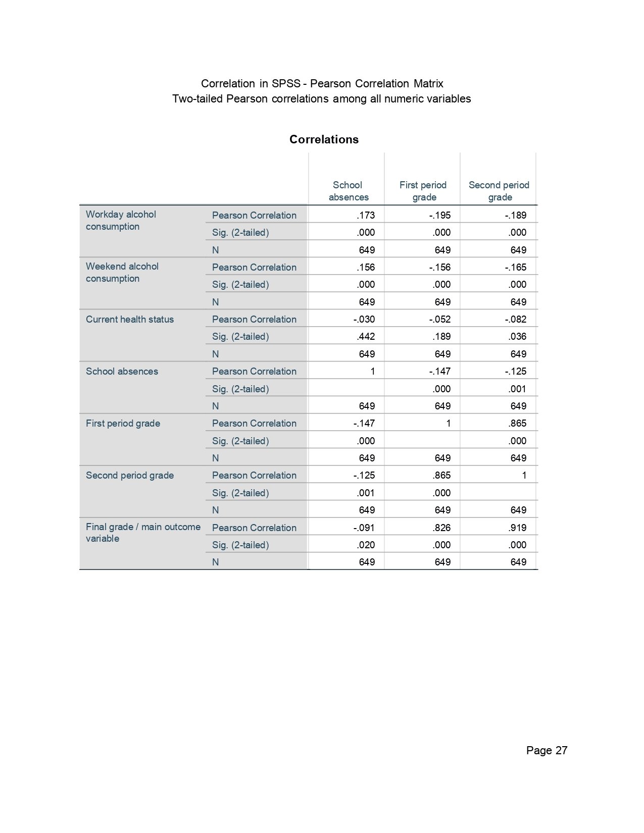
This page supports the diagnostic and reporting section of the SPSS output. A good correlation report should connect the visual pattern with the numeric matrix: the grades form a strong positive academic-performance cluster, while weaker background and behavior variables should not be overstated. Use this image to remind readers that a statistically significant correlation still needs a practical interpretation.
SPSS Output Image 22: Page 0028
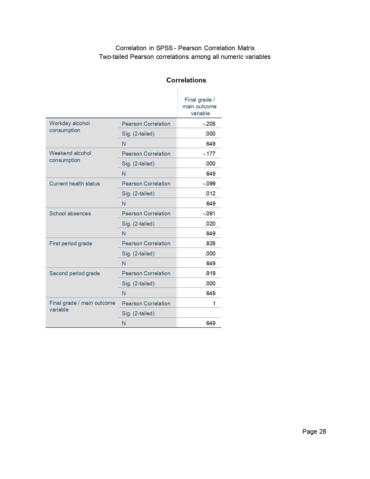
This page supports the diagnostic and reporting section of the SPSS output. A good correlation report should connect the visual pattern with the numeric matrix: the grades form a strong positive academic-performance cluster, while weaker background and behavior variables should not be overstated. Use this image to remind readers that a statistically significant correlation still needs a practical interpretation.
SPSS Output Image 23: Page 0030
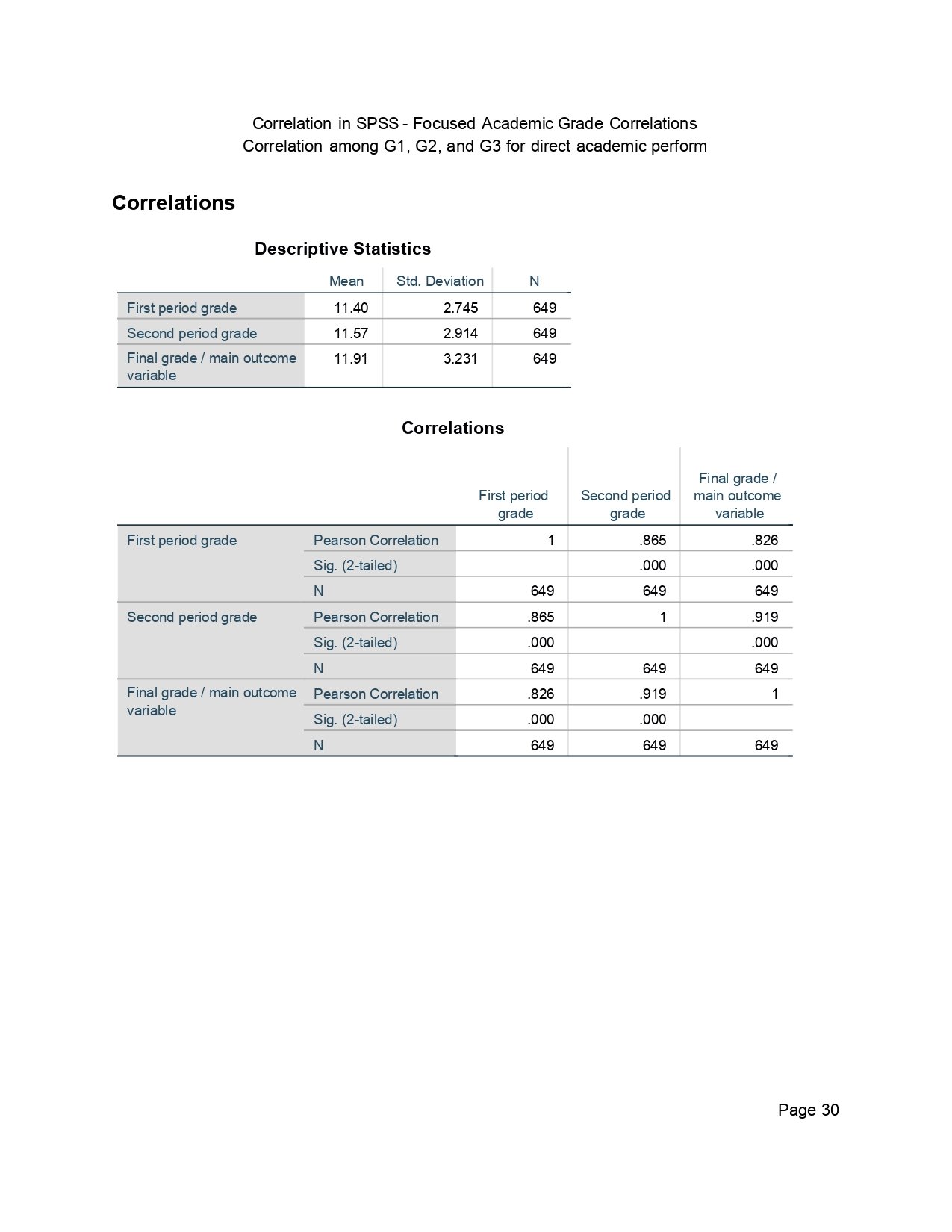
This page supports the diagnostic and reporting section of the SPSS output. A good correlation report should connect the visual pattern with the numeric matrix: the grades form a strong positive academic-performance cluster, while weaker background and behavior variables should not be overstated. Use this image to remind readers that a statistically significant correlation still needs a practical interpretation.
SPSS Output Image 24: Page 0032
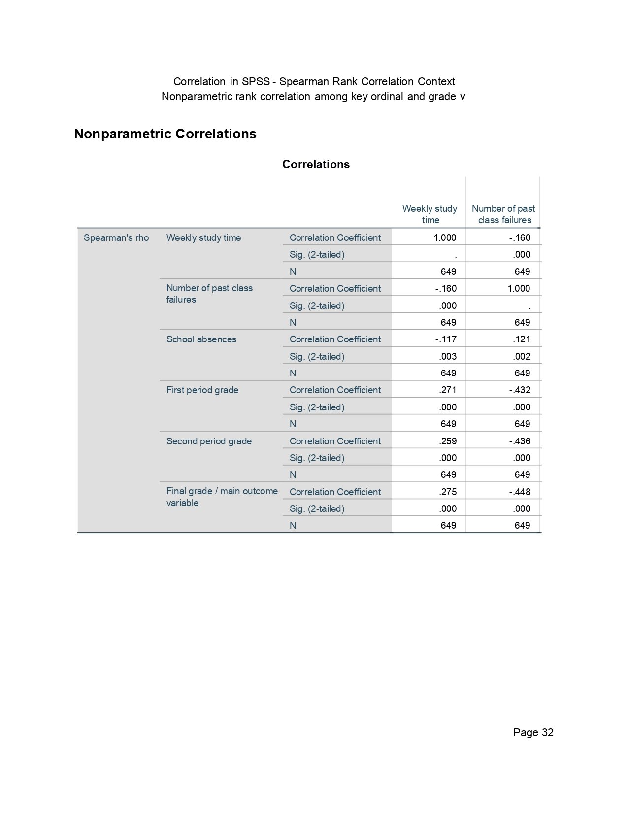
This later SPSS output image gives additional evidence from the exported Viewer pages. It is useful in the post because many readers want to compare the written interpretation with actual SPSS pages. The key reading habit is the same throughout: locate the variable pair, read Pearson’s r or Spearman’s rho, check the two-tailed significance value, and confirm the valid sample size.
SPSS Output Image 25: Page 0033
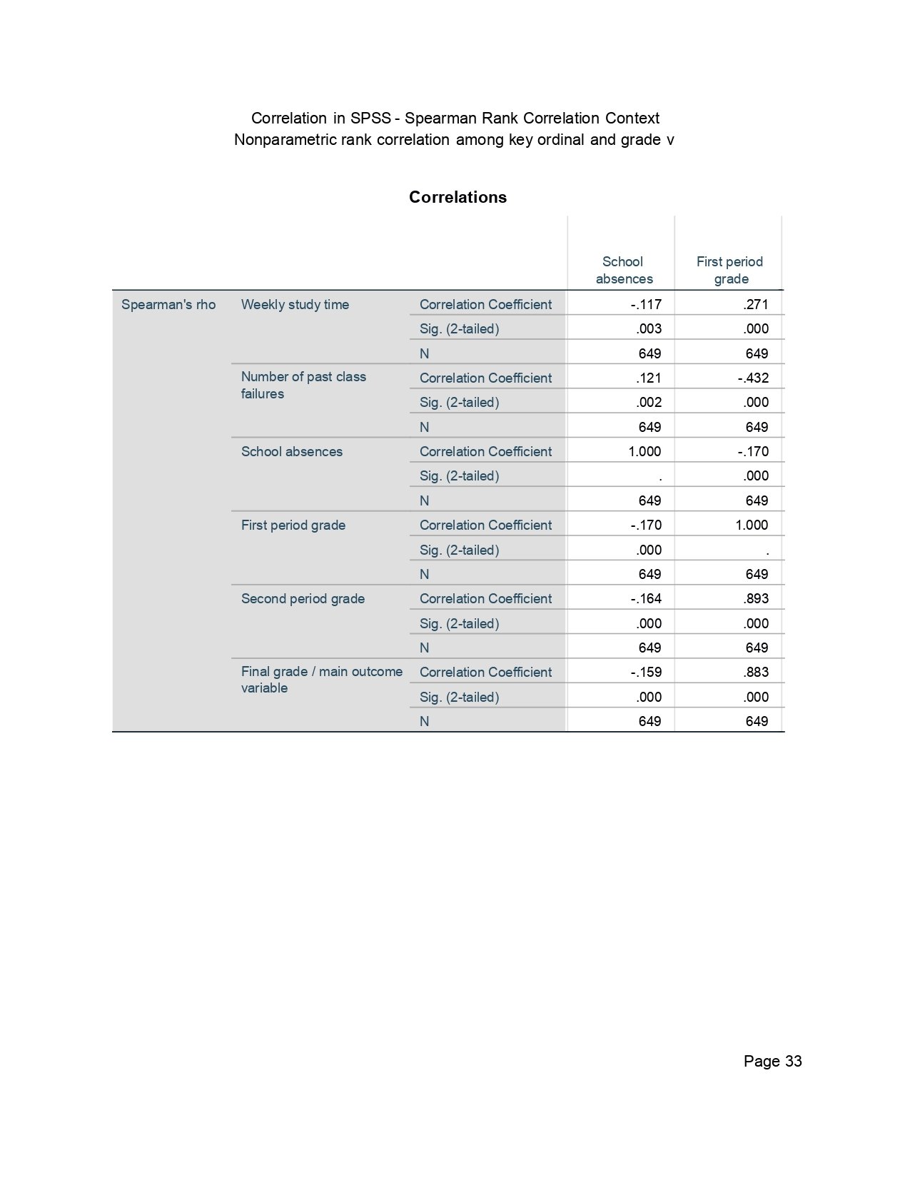
This later SPSS output image gives additional evidence from the exported Viewer pages. It is useful in the post because many readers want to compare the written interpretation with actual SPSS pages. The key reading habit is the same throughout: locate the variable pair, read Pearson’s r or Spearman’s rho, check the two-tailed significance value, and confirm the valid sample size.
SPSS Output Image 26: Page 0034
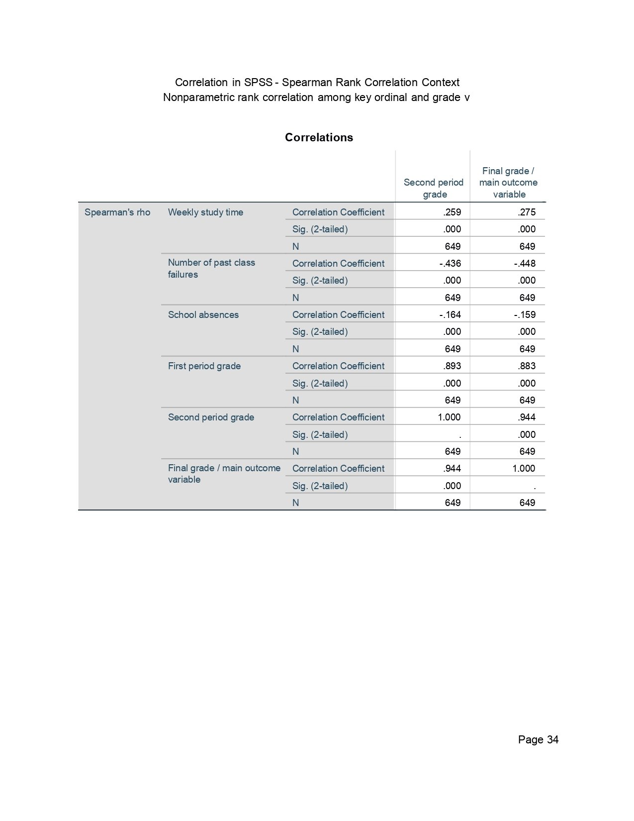
This later SPSS output image gives additional evidence from the exported Viewer pages. It is useful in the post because many readers want to compare the written interpretation with actual SPSS pages. The key reading habit is the same throughout: locate the variable pair, read Pearson’s r or Spearman’s rho, check the two-tailed significance value, and confirm the valid sample size.
SPSS Output Image 27: Page 0036
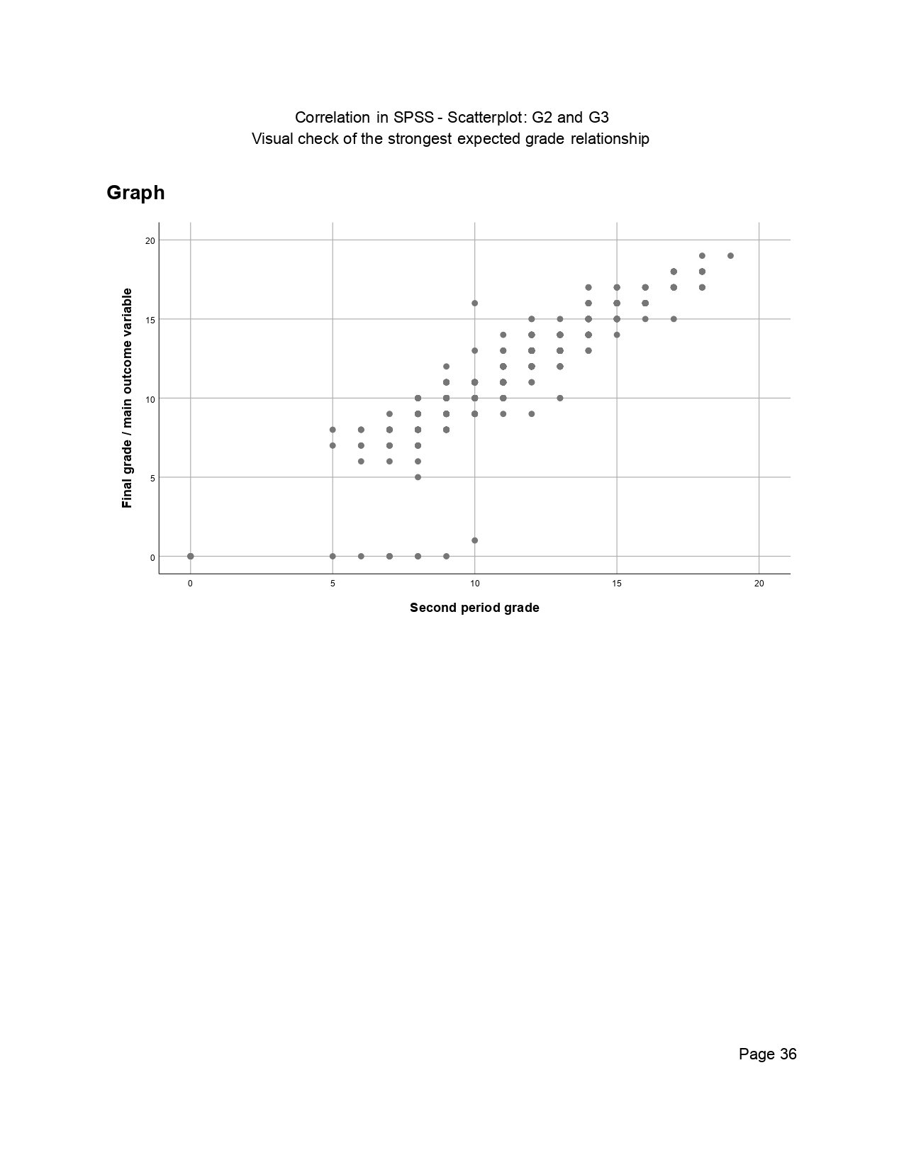
This later SPSS output image gives additional evidence from the exported Viewer pages. It is useful in the post because many readers want to compare the written interpretation with actual SPSS pages. The key reading habit is the same throughout: locate the variable pair, read Pearson’s r or Spearman’s rho, check the two-tailed significance value, and confirm the valid sample size.
SPSS Output Image 28: Page 0038
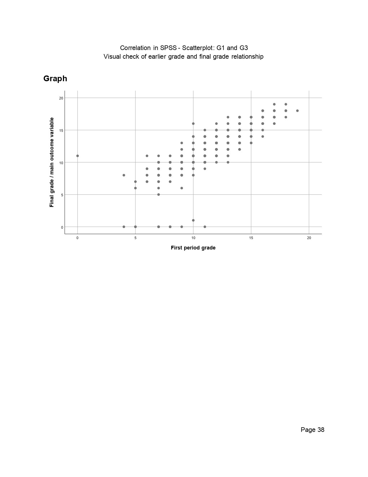
This final-group SPSS output page belongs to the closing part of the exported output. It helps show that the analysis was not limited to one table; the Viewer output includes multiple pages of tables, graphs, and supporting evidence. For the article conclusion, the most important result remains the strong positive G1–G2–G3 grade cluster, especially G2 with G3 at about r = .919.
SPSS Output Image 29: Page 0040
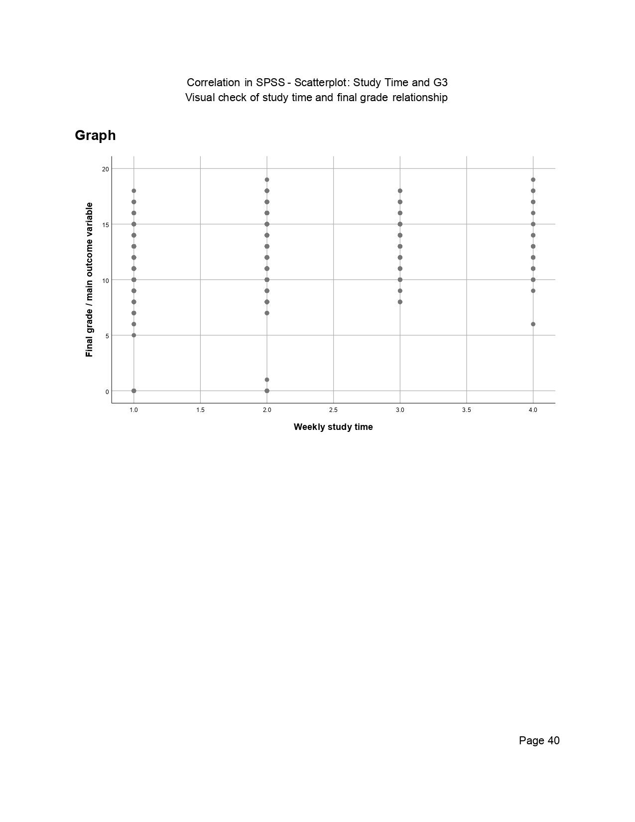
This final-group SPSS output page belongs to the closing part of the exported output. It helps show that the analysis was not limited to one table; the Viewer output includes multiple pages of tables, graphs, and supporting evidence. For the article conclusion, the most important result remains the strong positive G1–G2–G3 grade cluster, especially G2 with G3 at about r = .919.
SPSS Output Image 30: Page 0042
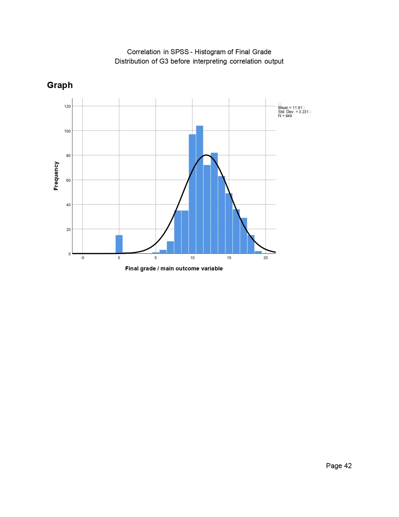
This final-group SPSS output page belongs to the closing part of the exported output. It helps show that the analysis was not limited to one table; the Viewer output includes multiple pages of tables, graphs, and supporting evidence. For the article conclusion, the most important result remains the strong positive G1–G2–G3 grade cluster, especially G2 with G3 at about r = .919.
Assumptions for Pearson Correlation in SPSS
Pearson correlation is easy to run, but it still has assumptions. Before reporting Pearson r, check whether the relationship is approximately linear, whether the variables are measured on a numeric scale, whether extreme outliers distort the result, and whether the pattern is meaningful rather than driven by a small number of observations.
| Assumption | How to Check in SPSS | What to Do If It Fails |
|---|---|---|
| Linearity | Create a scatterplot for the two variables. | Use Spearman correlation or model the relationship differently. |
| Numeric variables | Check Variable View and measurement level. | Use Spearman or another method for ordinal variables. |
| No serious outliers | Inspect scatterplots and boxplots. | Investigate outliers and report sensitivity checks. |
| Approximate normality for inference | Use histograms, Q-Q plots, and normality tests. | Use Spearman correlation when normality is poor. |
| Independent observations | Review the study design. | Use grouped or repeated-measures methods when observations are not independent. |
These assumptions connect with Shapiro-Wilk test, normal distribution, outlier detection, box plot interpretation, and influence diagnostics.
SPSS Syntax for Correlation
* Correlation in SPSS: Pearson and Spearman examples.
* Example variables: G1 G2 G3 studytime failures absences.

OUTPUT CLOSE ALL.
OUTPUT NEW NAME=Correlation_in_SPSS_Output.

DESCRIPTIVES VARIABLES=G1 G2 G3 studytime failures absences
  /STATISTICS=MEAN STDDEV MIN MAX.

CORRELATIONS
  /VARIABLES=G1 G2 G3 studytime failures absences
  /PRINT=TWOTAIL
  /MISSING=PAIRWISE.

NONPAR CORR
  /VARIABLES=G1 G2 G3 studytime failures absences
  /PRINT=SPEARMAN TWOTAIL
  /MISSING=PAIRWISE.

GRAPH
  /SCATTERPLOT(BIVAR)=G2 WITH G3.

GRAPH
  /SCATTERPLOT(BIVAR)=G1 WITH G3.

OUTPUT EXPORT
  /CONTENTS EXPORT=VISIBLE
  /PDF DOCUMENTFILE='Correlation-in-SPSS-Output.pdf'.
APA Reporting Wording for Correlation in SPSS
When writing a correlation result from SPSS, report the variable pair, correlation type, coefficient, p-value, N, direction, strength and practical interpretation. Do not report only “p < .05.” The coefficient is the actual effect size.
APA-Style Full Report
A Pearson product-moment correlation was computed to examine the relationship between G2 and G3. There was a very strong positive correlation between the two variables, r(647) = .919, p < .001, N = 649. Students with higher G2 scores tended to have higher G3 final scores. Additional strong positive correlations were observed between G1 and G2, r = .865, p < .001, and between G1 and G3, r = .826, p < .001.
Short APA-Style Version
G2 and G3 were very strongly and positively correlated, r(647) = .919, p < .001. This indicates that higher G2 scores were associated with higher final G3 scores.
Plain-Language Report Wording
The SPSS correlation output shows that the grade variables are closely connected. The strongest association is between G2 and G3, meaning students who performed well on G2 usually also performed well on the final grade measure. The relationship is strong and statistically significant, but it should still be described as an association rather than a causal effect.
Common Mistakes in Correlation in SPSS
| Mistake | Why It Is a Problem | Better Practice |
|---|---|---|
| Reading only Sig. (2-tailed) | The p-value does not show strength. | Report both r and p. |
| Ignoring the sign of r | Positive and negative correlations mean different things. | Explain direction clearly. |
| Calling correlation causal | SPSS correlation is not a causal test. | Use association language. |
| Using Pearson for every variable | Ordinal or non-normal variables may need Spearman. | Match the test to the data scale and assumptions. |
| Ignoring scatterplots | A coefficient can hide curvature or outliers. | Check visual patterns before reporting Pearson r. |
| Overreporting the full matrix | Large tables can overwhelm readers. | Summarize the key pairs and place the full table in the output file. |
Downloads and Resources
FAQs About Correlation in SPSS
How do I run correlation in SPSS?
Go to Analyze → Correlate → Bivariate, move your variables into the Variables box, select Pearson or Spearman, choose the significance option, and click OK.
What does Pearson Correlation mean in SPSS?
It is the correlation coefficient showing the strength and direction of a linear relationship between two numeric variables.
What does Sig. (2-tailed) mean in SPSS correlation?
Sig. (2-tailed) is the p-value for testing whether the population correlation differs from zero.
What does N mean in SPSS correlation output?
N is the number of valid paired observations used for that variable pair.
When should I use Spearman instead of Pearson in SPSS?
Use Spearman when variables are ordinal, the relationship is monotonic rather than linear, or Pearson assumptions are not suitable.
How do I report SPSS correlation in APA style?
Report the test type, variables, coefficient, degrees of freedom or N, p-value, direction, and interpretation. Example: G2 and G3 were strongly correlated, r(647) = .919, p < .001.
Does correlation in SPSS prove causation?
No. Correlation shows association, not cause-and-effect.

