
Cohen’s Kappa: Formula, Interpretation, Calculator, Python, R, SPSS and Excel Guide
Cohen’s Kappa measures agreement between two classifications after removing the agreement expected by chance from their marginal distributions. This complete guide explains what Cohen’s Kappa measures, the formula, assumptions, hand calculation, interpretation, negative values, weighted kappa, prevalence effects, calculator logic, Python, R, SPSS and Excel workflows, APA reporting, charts and downloads through a verified four-category grade-band analysis of 649 students.
491 exact agreements
Observed agreement 75.65%
Cohen’s κ = 0.6100
What Is Cohen’s Kappa?
Cohen’s Kappa, usually written as κ, is a chance-corrected coefficient of agreement for two raters, two observers, two diagnostic methods, two machine-learning classifiers or two classification occasions that assign the same cases to the same set of categorical outcomes. It belongs to the broader family of categorical-data methods discussed in cross-tabulation, frequency and relative frequency tables and categorical data analysis in Python.
Raw percent agreement answers a simple question: what proportion of paired classifications match exactly? Cohen’s Kappa asks a more demanding question: how much of that observed agreement remains after subtracting the agreement that would arise from the two marginal category distributions? This distinction matters whenever one or more categories are common, because high raw agreement can occur even when the raters or methods add little information beyond category prevalence.
What does Cohen’s Kappa measure?
Cohen’s Kappa measures the proportion of the maximum possible agreement beyond chance that was actually achieved. A kappa of 1 means perfect agreement. A kappa of 0 means observed agreement is exactly what the marginal distributions predict under chance independence. A negative value means observed agreement is worse than chance expectation. Because the coefficient is based on a two-way table, it should always be interpreted beside the agreement matrix, marginal proportions and category-specific patterns.
Worked example in this guide
The current analysis classifies 649 students into four grade bands twice: once from G1 and once from G2. The band rules are 1 = score below 10, 2 = score 10–13, 3 = score 14–16 and 4 = score 17–19. The two classification occasions are compared as nominal categories. Although the bands have a natural order, the verified primary analysis is unweighted Cohen’s Kappa, so every off-diagonal disagreement is treated equally. Weighted kappa is discussed later as a separate ordinal extension.
The null states that agreement beyond chance is zero. The alternative states that agreement differs from chance. For hypothesis wording and decision rules, see null and alternative hypothesis, p-value and type I and type II error.
Quick Answer: Cohen’s Kappa Result
The verified Excel, Python, R and SPSS outputs report the same nominal four-category agreement result.
Statistical summary
- Procedure: unweighted nominal Cohen’s Kappa
- Classifications: G1 grade band and G2 grade band
- Categories: four common bands
- κ: 0.6100175
- Approximate 95% CI: 0.5584 to 0.6616
- Decision: reject H0: κ = 0
Substantive meaning
- Three-quarters of classifications match exactly.
- Chance alone predicts agreement for about 37.6% of cases.
- Kappa retains about 61.0% of the possible agreement beyond chance.
- Most disagreements are between adjacent grade bands.
- The coefficient is substantial enough to be useful but not high enough to imply interchangeability without qualification.
Table of Contents
- Research question, design and hypotheses
- When to use Cohen’s Kappa
- Applications of Cohen’s Kappa
- Cohen’s Kappa formula and hand calculation
- Variables and grade-band coding
- Observed agreement matrix
- Complete Cohen’s Kappa results
- Cohen’s Kappa interpretation
- Kappa versus percent agreement
- Weighted kappa, Fleiss kappa and alternatives
- Prevalence, bias and negative kappa
- Cohen’s Kappa calculator steps
- Python chart interpretations
- R chart pairs and explanations
- Python, R, SPSS, Excel, SAS and Stata
- Expandable software code
- Assumptions and limitations
- APA reporting
- Worked practice questions
- Reports and Excel download
- Related Salar Cafe guides
- Frequently asked questions
- Conclusion
Research Question, Design and Hypotheses
Research question
How strongly do G1 and G2 agree when both scores are converted into the same four grade-band categories, after correcting raw agreement for chance agreement implied by the marginal category frequencies?
Null and alternative hypotheses
| Hypothesis | Statistical statement | Meaning |
|---|---|---|
| Null hypothesis | H0: κ = 0 | Observed agreement does not exceed marginal chance agreement. |
| Two-sided alternative | H1: κ ≠ 0 | Agreement differs from chance expectation. |
| Positive-agreement expectation | κ > 0 | Used descriptively when agreement above chance is expected, but the formal two-sided test remains transparent. |
Why this is an agreement question, not a correlation question
Correlation evaluates association or rank/linear co-movement; agreement asks whether paired classifications are the same. Two methods can correlate highly while disagreeing systematically. Conversely, categories can agree frequently without a meaningful linear relationship. See correlation versus regression, Pearson correlation and Spearman rank correlation for association-focused alternatives.
When to Use Cohen’s Kappa
Use Cohen’s Kappa when
- Exactly two raters, methods or classification occasions evaluate the same cases.
- Both use the same mutually exclusive category set.
- The response is nominal or binary for unweighted kappa.
- You need agreement corrected for chance rather than raw percent agreement alone.
- Each pair of classifications is independent of other case pairs.
- The rating table is complete enough for a meaningful cross-tabulation.
Choose another statistic when
- There are more than two raters; consider a multi-rater kappa such as Fleiss-type methods.
- The outcome is continuous; consider the intraclass correlation coefficient.
- The categories are ordered and disagreement distance matters; consider weighted kappa.
- You are testing association rather than agreement; consider chi-square test of independence.
- The paired table is square and you want marginal symmetry rather than agreement; consider Bowker’s Test of Symmetry.
- You need model-based adjustment for predictors; consider multinomial logistic regression or another classification model.
Binary versus multicategory Cohen’s Kappa
Cohen’s Kappa works with two categories or more than two categories. With binary data, the table is 2 × 2 and terms such as positive agreement, negative agreement, sensitivity and specificity may also matter. With multicategory data, the table is square with one row and one column per category. The current 4 × 4 analysis demonstrates the multicategory case.
Cohen’s Kappa in machine learning
In machine learning, Cohen’s Kappa can compare predicted classes with reference classes or compare two classifiers on the same observations. It is not identical to accuracy because it subtracts marginal chance agreement. However, kappa still depends on class prevalence and predicted marginals, so it should be interpreted with the confusion matrix and class-specific performance rather than used as the only model metric.
If no, choose a multi-rater or multi-method procedure.
If no, harmonize categories before agreement analysis.
If yes, use a justified weighting scheme rather than unweighted kappa.
Applications of Cohen’s Kappa
Compare two clinicians, two screening methods or a human assessment with a reference classification when outcomes are categorical.
Evaluate whether two coders assign news stories, interviews, social-media posts or documents to the same thematic categories.
Compare two grading occasions, two teachers or two categorical rubrics applied to the same students or assignments.
Compare predicted classes with reference labels or compare two classifiers on exactly the same observations.
Cohen’s Kappa in communication and content analysis
Communication researchers often use Cohen’s Kappa to quantify inter-coder reliability. Two coders independently classify the same messages, documents or media units into a common category system. The coefficient is meaningful only when the coding manual defines mutually exclusive categories and the coders evaluate the same units independently. A training phase can be used to refine definitions, but the final reliability sample should be coded without consultation.
Cohen’s Kappa in healthcare
Healthcare applications include agreement between radiologists, diagnostic tests, triage systems or categorical clinical ratings. High stakes require more than a generic label such as “substantial.” Report category prevalence, false-negative and false-positive patterns, confidence intervals and any clinically important disagreement. Agreement between two methods does not establish that either method is valid against a gold standard.
Cohen’s Kappa in machine learning versus accuracy and AUC
Accuracy is raw agreement between predictions and reference labels. Cohen’s Kappa adjusts that agreement for the prediction and reference marginals. AUC answers a different question: how well a scoring model ranks positive cases above negative cases across thresholds. Kappa is therefore a threshold- and category-dependent agreement metric, whereas AUC is a discrimination metric. Neither should replace the confusion matrix, class prevalence and application-specific error costs.
Cohen’s Kappa in education
In the present example, G1 and G2 are not two human raters; they are two classification occasions applied to the same students. Cohen’s Kappa is still applicable because the mathematical requirement is two paired categorical classifications using the same category set. This broader framing is useful when studying stability, repeatability or method agreement rather than only inter-rater reliability.
Cohen’s Kappa Formula and Hand Calculation
The formula compares observed exact agreement with expected chance agreement:
| Symbol | Definition | Worked value |
|---|---|---|
| N | Total paired classifications | 649 |
| Po | Observed exact-agreement proportion | 491/649 = 0.7565485 |
| Pe | Expected agreement from row and column marginals | 0.3757375 |
| 1 − Pe | Maximum possible agreement beyond chance | 0.6242625 |
| Po − Pe | Observed agreement above chance | 0.3808111 |
| κ | Proportion of possible beyond-chance agreement achieved | 0.6100175 |
Step 1: Add the diagonal agreements
Step 2: Calculate marginal proportions
For G1, the row totals are 157, 340, 128 and 24. For G2, the column totals are 145, 352, 117 and 35. Divide each total by 649 to obtain marginal proportions.
| Band | G1 marginal | G2 marginal | Chance-agreement component |
|---|---|---|---|
| 1: below 10 | 157/649 = 0.2419106 | 145/649 = 0.2234206 | 0.0540478 |
| 2: 10–13 | 340/649 = 0.5238829 | 352/649 = 0.5423729 | 0.2841399 |
| 3: 14–16 | 128/649 = 0.1972265 | 117/649 = 0.1802773 | 0.0355555 |
| 4: 17–19 | 24/649 = 0.0369800 | 35/649 = 0.0539291 | 0.0019943 |
Step 3: Sum expected chance-agreement components
Equivalently, the expected diagonal counts are approximately 35.077, 184.407, 23.076 and 1.294, totalling 243.854 expected chance agreements.
Step 4: Substitute into the kappa formula
Step 5: Test whether kappa differs from zero
The verified output gives z = 23.1776 and a two-sided p-value of 7.6555 × 10−119. The implied standard error is approximately 0.02632, producing a normal-approximation 95% confidence interval of about 0.5584 to 0.6616. For interval concepts, see standard error, confidence interval formula and margin of error and confidence level.
Variables and Grade-Band Coding
| Variable | Role | Original scale | Derived categories | Interpretation |
|---|---|---|---|---|
| G1 | First classification occasion | Grade score 0–19 | Band 1 <10; Band 2 = 10–13; Band 3 = 14–16; Band 4 = 17–19 | Row classification in the agreement matrix. |
| G2 | Second classification occasion | Grade score 0–19 | Same four thresholds | Column classification in the agreement matrix. |
| Student | Paired unit | One row per student | N = 649 | Links the two classifications for agreement analysis. |
Why identical categories are required
Both classification occasions must use the same category definitions. If G1 used different cut points from G2, diagonal cells would no longer represent the same substantive category. Category harmonization is therefore a design requirement, not a cosmetic data-cleaning step. See categorical and quantitative variables and descriptive statistics for coding foundations.
Nominal treatment despite ordinal bands
The four grade bands are ordered, but the primary workbook deliberately treats them as nominal. Therefore, a disagreement from Band 1 to Band 2 receives the same penalty as a disagreement from Band 1 to Band 4. This is appropriate for an unweighted kappa demonstration and provides a conservative, transparent exact-match analysis. If severity of disagreement matters, weighted kappa should be prespecified and reported separately.
Observed Cohen’s Kappa Agreement Matrix
| G1 band \ G2 band | 1: <10 | 2: 10–13 | 3: 14–16 | 4: 17–19 | G1 row total |
|---|---|---|---|---|---|
| 1: <10 | 107 | 50 | 0 | 0 | 157 |
| 2: 10–13 | 38 | 274 | 27 | 1 | 340 |
| 3: 14–16 | 0 | 28 | 88 | 12 | 128 |
| 4: 17–19 | 0 | 0 | 2 | 22 | 24 |
| G2 column total | 145 | 352 | 117 | 35 | 649 |
Diagonal and off-diagonal meaning
The diagonal cells 107, 274, 88 and 22 are exact agreements. The 158 off-diagonal cases are disagreements. Most disagreements are adjacent: 50 move from G1 Band 1 to G2 Band 2, 38 move from G1 Band 2 to G2 Band 1, 27 move from Band 2 to Band 3, 28 move from Band 3 to Band 2, 12 move from Band 3 to Band 4 and 2 move from Band 4 to Band 3. Only one case moves from Band 2 to Band 4, and no cases make the largest possible Band 1↔Band 4 jump.
Why adjacent disagreement matters
Unweighted Cohen’s Kappa correctly counts every off-diagonal cell as disagreement, but it does not distinguish small and large errors. The concentration of disagreements near the diagonal indicates that a weighted analysis could produce a higher coefficient because one-band differences would receive less penalty than distant differences. That does not invalidate the unweighted result; it answers a different question.
Complete Cohen’s Kappa Results
491 of 649
243.854 expected cases
Po − Pe
Unweighted nominal κ
Test against κ = 0
Two-sided
| Result | Estimate | Interpretation |
|---|---|---|
| Exact agreement count | 491 | Number of paired classifications on the matrix diagonal. |
| Observed disagreement | 0.2434515 | 24.35% of pairs do not match exactly. |
| Expected disagreement | 0.6242625 | Chance model expects 62.43% disagreement. |
| Cohen’s Kappa | 0.6100175 | 61.00% of possible beyond-chance agreement was achieved. |
| Approximate 95% CI | 0.5584 to 0.6616 | Precision range from the reported normal approximation. |
| Significance test | z = 23.1776, p ≈ 7.66 × 10−119 | Agreement is decisively greater than chance. |
Statistical interpretation
The p-value is far below .05, .01 and .001, so the null of zero chance-corrected agreement is rejected. Statistical significance is unsurprising with 649 paired cases and κ above .60. The more useful questions are how large the agreement is, where disagreements occur and whether unweighted exact agreement matches the practical purpose.
Practical interpretation
The G1 and G2 band classifications match exactly for roughly three of every four students. After removing the 37.57% chance agreement predicted by the marginal category frequencies, the coefficient is .610. This indicates useful stability between classification occasions but leaves meaningful room for change or disagreement. Because many disagreements are only one band apart, users should not describe the two classifications as unreliable solely because 24.35% are off the diagonal.
Cohen’s Kappa Interpretation
There is no universal interpretation scale that overrides context. Common descriptive labels can help readers orient themselves, but they are conventions rather than laws. A coefficient acceptable for exploratory coding may be too low for a high-stakes diagnosis, legal decision or safety-critical classification.
| Kappa range | Common descriptive label | Reporting caution |
|---|---|---|
| κ < 0 | Worse than chance | Check coding, systematic reversal, category definitions and data pairing. |
| 0.00–0.20 | Slight agreement | May be inadequate unless the task is highly noisy or exploratory. |
| 0.21–0.40 | Fair agreement | Interpret with category-specific disagreement and confidence intervals. |
| 0.41–0.60 | Moderate agreement | Potentially useful, but not necessarily sufficient for interchangeability. |
| 0.61–0.80 | Substantial agreement | Strong descriptive agreement, still requiring context and table review. |
| 0.81–1.00 | Almost perfect agreement | High agreement, but verify prevalence, bias and sample representativeness. |
The worked κ = 0.6100 lies almost exactly at the boundary between commonly labelled moderate and substantial agreement. It is better to report the numeric estimate, confidence interval, raw agreement and context than to argue over a boundary label. For broader magnitude reasoning, compare effect size, Cramer’s V, phi coefficient and contingency coefficient.
What is a good Cohen’s Kappa value?
A good value is one that meets the consequences and reliability requirements of the application. In a low-risk exploratory study, κ around .60 may be useful. In a clinical, safety or certification decision, κ around .60 may be insufficient. The minimum acceptable value should be defined before analysis whenever possible, supported by subject-matter standards and accompanied by a confidence interval.
Do not confuse Cohen’s Kappa with Cohen’s d
Cohen’s Kappa is an agreement coefficient for categorical classifications. Cohen’s d is a standardized mean difference for quantitative outcomes. They answer different questions, use different formulas and are not interchangeable. For quantitative group comparisons, see two-sample t test and effect size.
Cohen’s Kappa Versus Percent Agreement
Diagonal count divided by N. Easy to explain but ignores agreement expected from marginals.
Chance-corrected agreement using observed and expected agreement.
Tests whether row and column classifications are associated, not whether they match exactly.
Measures association or co-movement, not exact categorical concordance.
Why 75.65% agreement becomes κ = .610
The raw agreement of 75.65% looks high, but the marginal distributions are concentrated in Band 2. Even unrelated classifications with the same marginals would agree about 37.57% of the time. Kappa subtracts this expected component and scales the remaining agreement against the maximum possible agreement beyond chance.
When percent agreement still matters
Kappa should not replace percent agreement. Raw agreement is directly interpretable and helps reveal whether a statistically respectable kappa is built from a practically acceptable match rate. Report both. For binary outcomes, positive and negative agreement may also be more informative than a single overall percentage.
Weighted Kappa, Fleiss Kappa and Other Alternatives
| Method | Use when | Key distinction |
|---|---|---|
| Unweighted Cohen’s Kappa | Two classifications with nominal categories | All disagreements receive equal penalty. |
| Weighted Cohen’s Kappa | Two classifications with ordered categories | Disagreements receive weights based on distance. |
| Fleiss-type kappa | More than two raters, often with varying raters per item | Extends chance-corrected agreement beyond two fixed raters. |
| Intraclass correlation | Continuous or ordered numeric measurements | Evaluates measurement agreement or consistency on quantitative scales. |
| Bowker’s symmetry test | Paired square categorical table | Tests whether off-diagonal flows are symmetric, not overall agreement strength. |
| Chi-square independence | Two categorical variables on observations | Tests association, not exact agreement. |
Why weighted kappa is relevant here
The grade bands are ordinal, and almost all disagreements are adjacent. A one-band disagreement is arguably less serious than a three-band disagreement. Weighted kappa can incorporate that reasoning through linear or quadratic weights. However, the weight system must be justified before viewing results because changing weights changes the coefficient.
Why the primary result remains unweighted
The uploaded workbook explicitly defines the categories as nominal for this analysis. The public post therefore preserves the verified unweighted κ = .6100 rather than replacing it with a different statistic. Weighted kappa belongs in a distinct sensitivity or extension section, not as an undocumented substitution.
Kappa versus ICC
If G1 and G2 are analysed as original quantitative scores rather than grade bands, the intraclass correlation coefficient guide is more directly relevant. Kappa is appropriate for the derived categorical classifications; ICC is appropriate for quantitative measurement agreement under a chosen ICC model.
Prevalence, Bias and Negative Cohen’s Kappa
The prevalence effect
When one category dominates, raw agreement may be high because both classifiers frequently choose that category. Expected chance agreement also becomes high, which can lower kappa. This is sometimes called a kappa prevalence paradox. It is not a computational mistake; it is a consequence of the marginal-based chance model.
The bias effect
If the two classifiers use categories at different rates, the marginal profiles differ. Depending on the table, marginal bias can increase or decrease kappa. In the worked example, the G1 and G2 marginal profiles are similar but not identical: Band 1 is 24.19% versus 22.34%, Band 2 is 52.39% versus 54.24%, Band 3 is 19.72% versus 18.03% and Band 4 is 3.70% versus 5.39%.
Can Cohen’s Kappa be negative?
Yes. κ becomes negative when observed agreement is less than expected agreement. A negative coefficient can result from systematic reversal, inconsistent category definitions, data-pairing errors or genuinely antagonistic classification. Before interpreting a negative result substantively, audit coding, case alignment and category order.
Can Cohen’s Kappa exceed 1?
No. The theoretical upper limit is 1. The lower limit can be below −1 only under malformed calculation; valid kappa values are bounded above by 1 and have a table-dependent minimum that is often greater than −1. Software returning a value outside the feasible range signals an implementation or data problem.
Cohen’s Kappa Calculator: Step-by-Step Workflow
A reliable Cohen’s Kappa calculator must accept the full square agreement table or paired category columns, not only the total number of agreements. Chance agreement cannot be computed without marginal category totals.
Calculator inputs for the worked example
| Input | Worked value | Purpose |
|---|---|---|
| Number of categories | 4 | Defines the square table dimensions. |
| Paired cases | 649 | Total observations classified twice. |
| Agreement matrix | [[107,50,0,0],[38,274,27,1],[0,28,88,12],[0,0,2,22]] | Provides diagonal and marginal counts. |
| Weighting | None | Requests unweighted nominal kappa. |
| Confidence level | 95% | Used for uncertainty reporting when supported. |
| Null value | κ = 0 | Tests agreement above chance. |
Calculator validation targets
- Diagonal agreement count should equal 491.
- Observed agreement should equal 0.7565485.
- Expected agreement should equal 0.3757375.
- Unweighted Cohen’s Kappa should equal 0.6100175.
- The result should not change if both raters’ category order is rearranged identically.
- The result may change if only one rater’s category order or coding is changed.
Excel calculator logic
In Excel, use the sum of diagonal cells divided by the grand total for Po. Multiply each row proportion by its corresponding column proportion and sum those products for Pe. Then apply the kappa formula. The supplied worked workbook already includes these calculations and formula checks.
Six Python Cohen’s Kappa Chart Interpretations
The Python workflow visualizes the agreement matrix, expected chance counts, category agreement, marginal distributions, agreement components and final result. These charts support the numeric analysis rather than replacing it.
Chart 1: Agreement MatrixPython
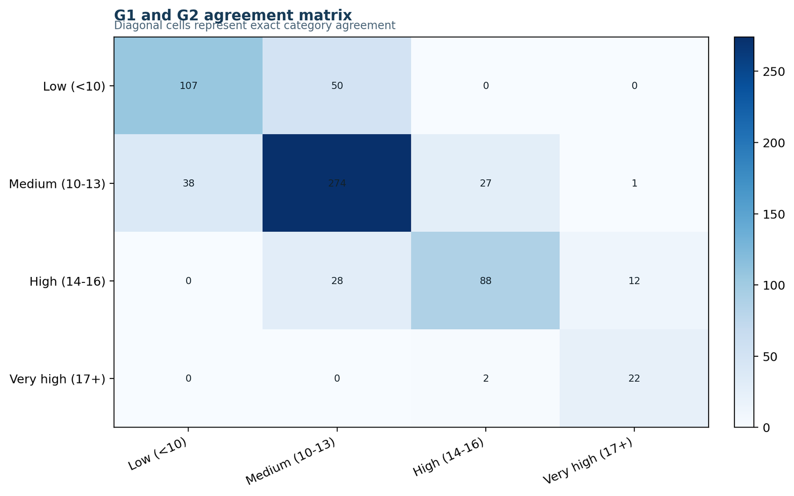
The largest cell is the Band 2 exact agreement, and most off-diagonal counts lie immediately beside the diagonal.
Exact matches are 107, 274, 88 and 22; total exact agreement is 491. The largest disagreements are 50 for Band 1→2 and 38 for Band 2→1.
Agreement is strong overall, while disagreements are mostly small shifts between neighbouring grade bands.
The matrix reveals where kappa comes from and shows why an ordinal weighted extension could be informative.
Chart 2: Chance-Expected Agreement CountsPython
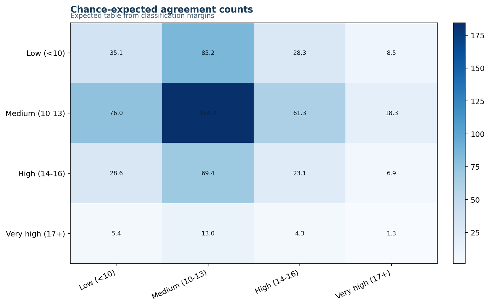
Band 2 contributes most of the chance agreement because it is the dominant category for both classifications.
Expected counts are about 35.08, 184.41, 23.08 and 1.29, totalling 243.85 expected agreements.
Observed diagonal counts exceed chance counts in every category, especially Bands 1, 2 and 3.
Kappa depends on expected agreement, so dominant categories can strongly affect the coefficient even when raw agreement is high.
Chart 3: Category-Specific Exact AgreementPython
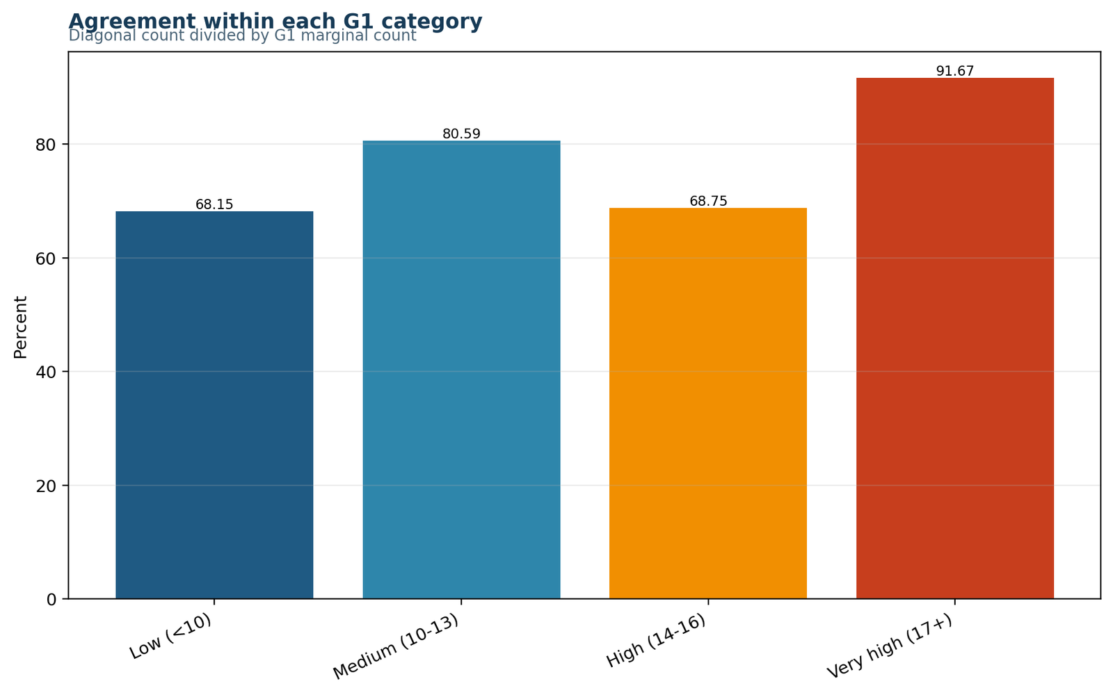
Band 2 contributes the largest number of exact matches because more than half of observations are classified in that band.
Diagonal counts are 107, 274, 88 and 22; their shares of the full sample are 16.49%, 42.22%, 13.56% and 3.39%.
A large category can dominate total agreement, so category-specific interpretation prevents the overall coefficient from hiding uneven performance.
Users may need separate agreement diagnostics for rare and common categories, particularly when rare categories are important.
Chart 4: Marginal DistributionsPython
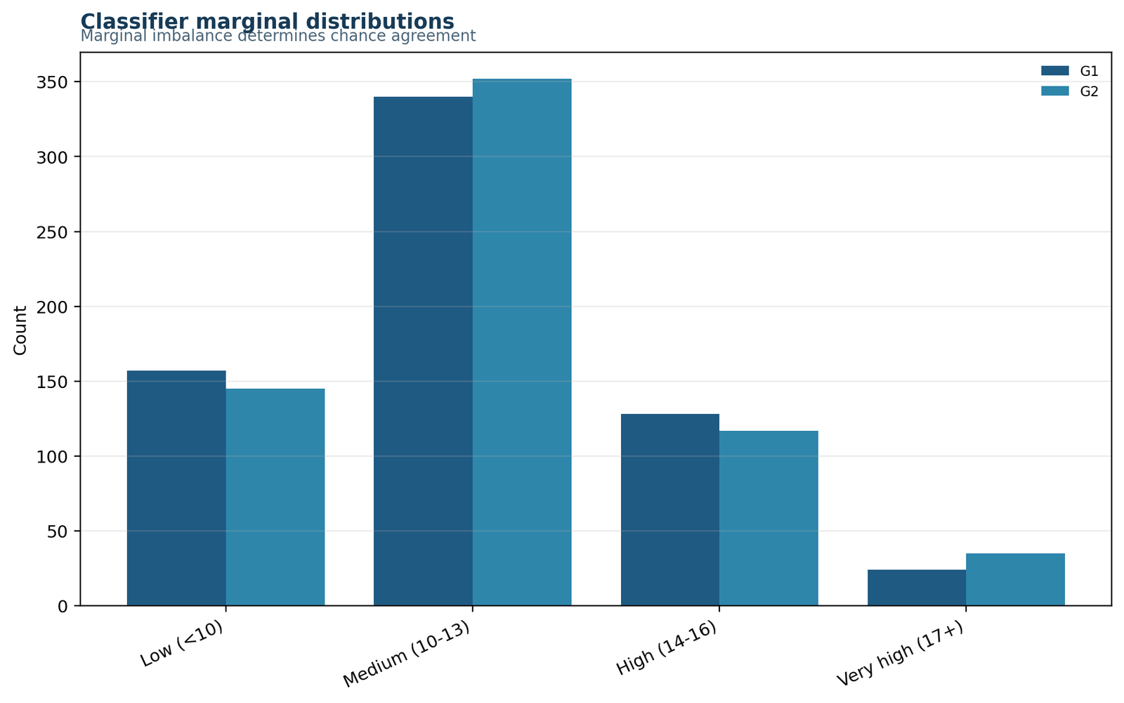
The two marginal profiles are similar, with Band 2 dominant and Band 4 rare, but G2 uses Band 4 somewhat more often.
G1 proportions are 24.19%, 52.39%, 19.72% and 3.70%; G2 proportions are 22.34%, 54.24%, 18.03% and 5.39%.
Similar marginals support a straightforward agreement interpretation, while small differences explain directional off-diagonal flows.
Marginal distributions determine P_e and can create prevalence or bias effects in kappa.
Chart 5: Observed and Expected Agreement ComponentsPython
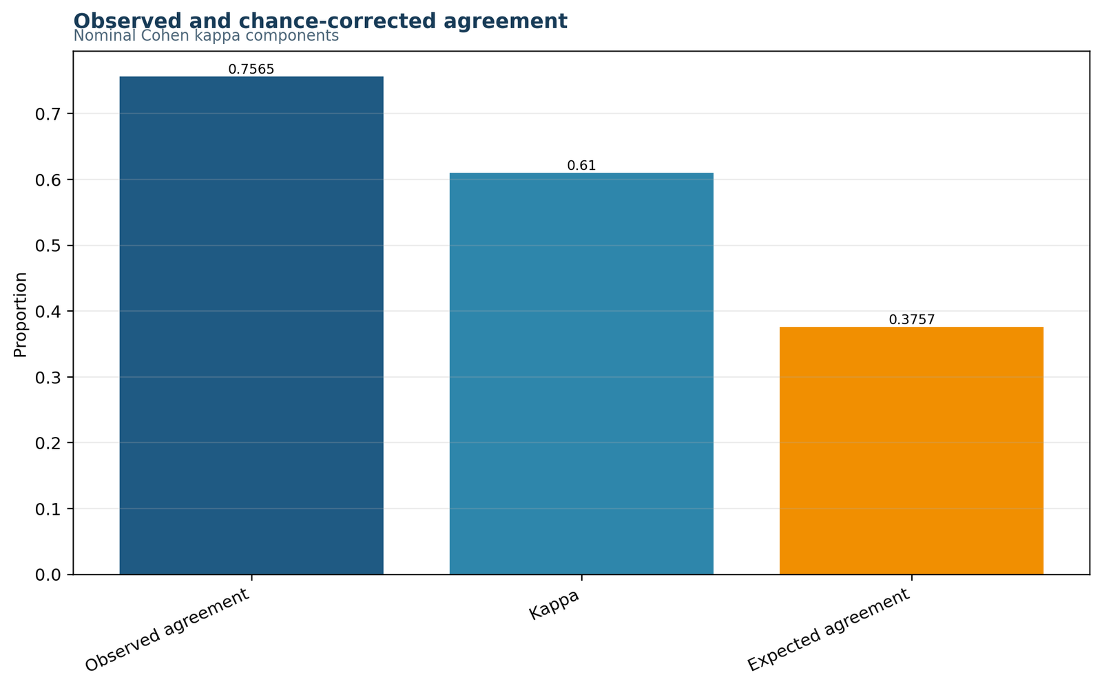
Observed agreement is roughly double expected chance agreement, leaving a substantial positive gap.
P_o = 0.75655, P_e = 0.37574, P_o − P_e = 0.38081 and 1 − P_e = 0.62426.
Kappa scales the 0.38081 observed advantage by the 0.62426 maximum available advantage.
This chart makes the formula intuitive and explains why κ is lower than raw percent agreement.
Chart 6: Cohen’s Kappa Result SummaryPython
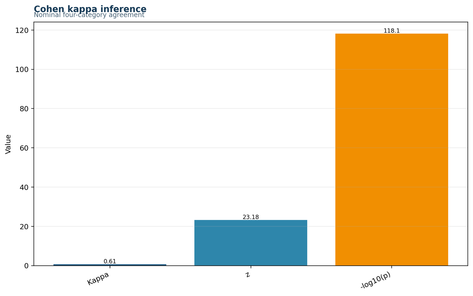
The coefficient is positive and far from zero, with a highly significant test result.
κ = 0.6100, observed agreement = 75.65%, expected agreement = 37.57%, z = 23.18 and p ≈ 7.66 × 10⁻119.
The two classifications show useful agreement beyond chance but are not perfectly interchangeable.
A compact result chart is useful for presentation, but the matrix and marginal charts remain necessary for diagnosis.
R Cohen’s Kappa Chart Pairs
The R workflow reproduces the same agreement structure in three paired rows. Each pair combines a visual diagnostic with a dedicated explanation so the reader can move from counts to marginals and then to the final coefficient.
R pair 1: Agreement matrix and expected agreement
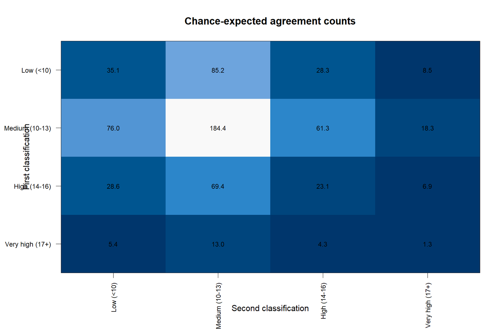
Exact agreement dominates the diagonal
The matrix contains 491 diagonal cases and 158 disagreements. The largest diagonal cell is Band 2 with 274 matches, reflecting both genuine stability and high prevalence.
Chance expectation is concentrated in Band 2
Band 2 alone contributes about 184.41 expected agreements because both marginals assign more than half the cases to that category. Expected agreement across all categories is 243.85 cases or 37.57%.
R pair 2: Diagonal agreement and marginal profiles
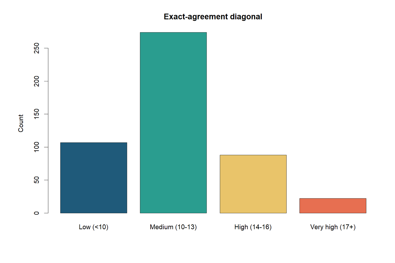
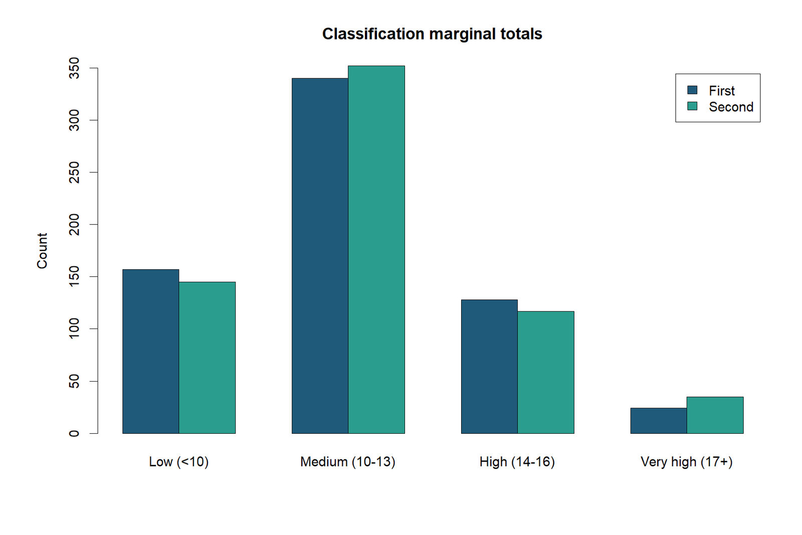
Agreement counts reflect prevalence
Band 2 produces the most exact matches, while Band 4 produces the fewest. This does not mean Band 4 is necessarily less reliable; it is also much rarer.
Marginals are similar but not identical
G2 assigns slightly fewer cases to Bands 1 and 3 and slightly more to Bands 2 and 4. These shifts contribute to directional disagreement and the chance-agreement calculation.
R pair 3: Observed versus expected agreement and result summary
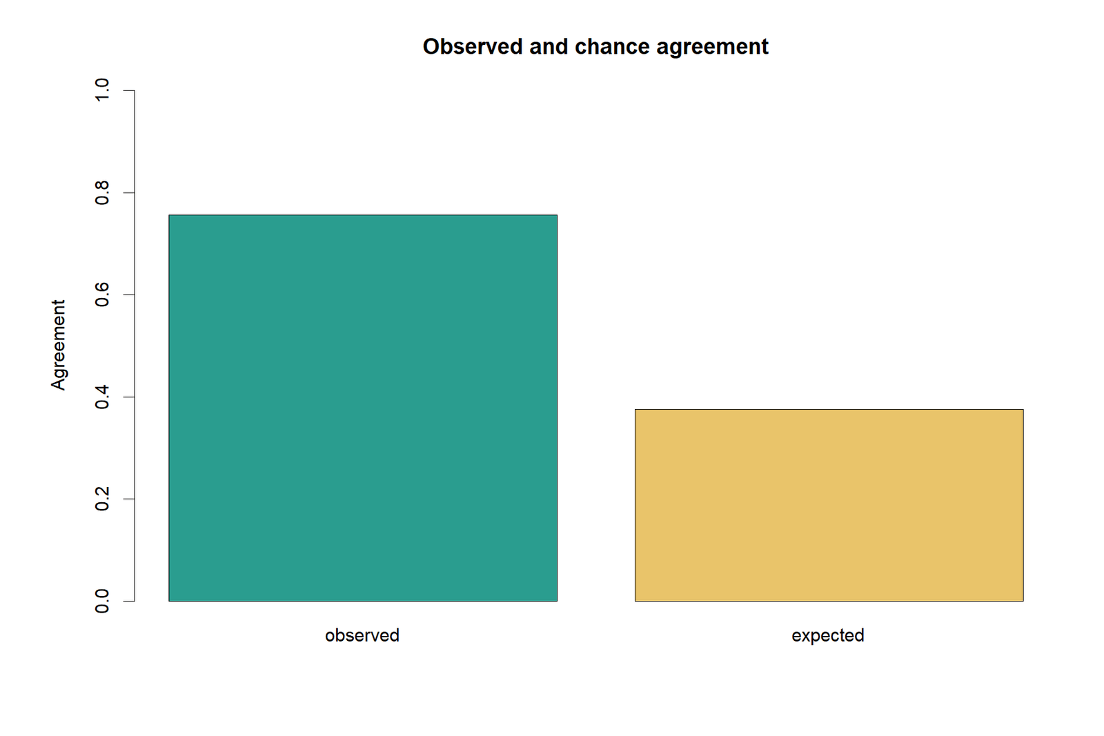
Observed agreement substantially exceeds chance
The 75.65% observed agreement is more than twice the 37.57% expected agreement. The difference of 38.08 percentage points supplies the numerator of kappa.
The final decision is decisive
The result summary reports κ = .6100 and an extremely small p-value. Agreement is clearly above chance, but the coefficient remains below 1 because 158 pairs disagree.
Cohen’s Kappa in Python, R, SPSS, Excel, SAS and Stata
Cohen’s Kappa in Python
Python can compute unweighted or weighted kappa from paired category vectors. The analysis should preserve the same category order in both vectors and explicitly state the weighting option. See categorical data analysis in Python and correlation in Python for related workflow conventions.
- Read G1 and G2.
- Apply identical band thresholds.
- Build the confusion/agreement matrix.
- Compute unweighted κ.
- Calculate P_o, P_e, marginals and uncertainty separately for transparent reporting.
Cohen’s Kappa in R
R offers agreement functions in several packages. The analyst should verify whether the function expects a matrix or paired vectors and whether the reported standard error uses asymptotic or bootstrap logic. See categorical data analysis in R and correlation in R.
- Create factors with identical levels.
- Cross-tabulate G1 band by G2 band.
- Request unweighted nominal kappa.
- Check the observed table and marginal proportions.
- Report package, version and confidence-interval method.
Cohen’s Kappa in SPSS
SPSS computes Cohen’s Kappa through Crosstabs when the two variables use the same category set. Place one classification in rows and the other in columns, request Kappa, and display observed counts. See categorical data analysis in SPSS and correlation in SPSS.
- Analyze → Descriptive Statistics → Crosstabs.
- Put G1 band in rows and G2 band in columns.
- Statistics → Kappa.
- Cells → observed counts and percentages.
- Export the table and symmetric-measures output.
Cohen’s Kappa in Excel
Excel can reproduce every component directly from the agreement table. The supplied workbook includes the paired input, observed matrix, calculations, marginal diagnostics and reporting sheet.
- Use COUNTIFS to build the 4 × 4 matrix.
- Sum the diagonal for observed agreement.
- Calculate row and column totals.
- Sum products of matching marginal proportions for expected agreement.
- Apply κ = (P_o − P_e)/(1 − P_e).
Cohen’s Kappa in SAS
SAS users can obtain kappa from frequency-table procedures when two categorical ratings are cross-classified. State whether simple or weighted agreement is requested, preserve category ordering and output the agreement table for verification.
- Prepare one record per paired case.
- Request the two-way table.
- Request agreement/kappa statistics.
- Use weights only when ordinal penalties are justified.
- Capture output through ODS for reproducibility.
Cohen’s Kappa in Stata
Stata provides commands for agreement between two categorical variables. Verify whether the command returns simple or weighted kappa and inspect marginal distributions before interpreting the coefficient.
- Encode both classifications consistently.
- Tabulate the paired categories.
- Run the kappa command.
- Request weights only for ordered categories.
- Report raw agreement and the coefficient together.
Expandable Cohen’s Kappa Code
Python example
import pandas as pd
from sklearn.metrics import cohen_kappa_score, confusion_matrix

# df contains original G1 and G2 scores.
bins = [-float("inf"), 9, 13, 16, float("inf")]
labels = [1, 2, 3, 4]
df["G1_band"] = pd.cut(df["G1"], bins=bins, labels=labels)
df["G2_band"] = pd.cut(df["G2"], bins=bins, labels=labels)

matrix = confusion_matrix(df["G1_band"], df["G2_band"], labels=labels)
kappa = cohen_kappa_score(df["G1_band"], df["G2_band"])
print(matrix)
print(kappa)
R example
breaks <- c(-Inf, 9, 13, 16, Inf)
labels <- c("1", "2", "3", "4")
df$G1_band <- cut(df$G1, breaks = breaks, labels = labels)
df$G2_band <- cut(df$G2, breaks = breaks, labels = labels)

tab <- table(df$G1_band, df$G2_band)
# Use a validated agreement package/function for unweighted kappa.
print(tab)
SPSS syntax example
* Derive common grade bands.
RECODE G1 G2 (Lowest thru 9=1) (10 thru 13=2) (14 thru 16=3) (17 thru Highest=4)
 INTO G1_band G2_band.

CROSSTABS
 /TABLES=G1_band BY G2_band
 /STATISTICS=KAPPA
 /CELLS=COUNT ROW COLUMN.
Excel formula outline
Observed agreement:
=SUM(diagonal_cells)/grand_total

Expected agreement:
=SUMPRODUCT(row_totals/grand_total,column_totals/grand_total)

Cohen's kappa:
=(observed_agreement-expected_agreement)/(1-expected_agreement)Cohen’s Kappa Assumptions and Limitations
Core assumptions
- The same cases are classified twice.
- Each case belongs to one category per classification.
- The two classifications use the same category definitions.
- Case pairs are independent of other case pairs.
- The categories are treated as nominal for unweighted kappa.
- Missing pairs are handled consistently.
Limitations
- Kappa depends on marginal prevalence.
- One coefficient can hide category-specific weakness.
- Unweighted kappa ignores disagreement distance.
- Statistical significance can be trivial with large N.
- Interpretation labels are context-dependent.
- Kappa does not identify the cause of disagreement.
Independence of cases
The two ratings within a student are deliberately dependent, but different students should be independent. If students are clustered within schools, classrooms or raters, standard asymptotic uncertainty may understate dependence. The agreement coefficient may still be descriptively useful, but inference may need cluster-aware resampling or modelling.
Missing classifications
Complete-case kappa uses only cases with both classifications observed. If missingness is related to category or disagreement, complete-case results can be biased. Report the number of excluded pairs and compare marginal distributions before and after exclusion. For sampling concerns, see sampling methods and sampling bias.
Do not infer validity from agreement
Two classifiers can agree with each other and both be wrong relative to a gold standard. Cohen’s Kappa evaluates reliability or concordance, not criterion validity. When a reference standard exists, examine accuracy, sensitivity, specificity and class-specific errors in addition to inter-method agreement.
APA Reporting for Cohen’s Kappa
Concise APA result
Agreement between G1 and G2 four-category grade-band classifications was assessed with unweighted Cohen’s Kappa. The classifications agreed for 491 of 649 students (75.65%), and agreement was significantly greater than chance, κ = .61, 95% CI [.56, .66], p < .001.
Expanded APA interpretation
An unweighted Cohen’s Kappa analysis evaluated exact agreement between G1 and G2 grade bands for 649 students. Observed agreement was 75.65%, compared with 37.57% agreement expected from the marginal distributions. The resulting coefficient indicated moderately strong chance-corrected agreement, κ = .610, 95% CI [.558, .662], z = 23.18, p < .001. Most disagreements occurred between adjacent grade bands.
Methods wording
G1 and G2 scores were converted to four identical grade bands: below 10, 10–13, 14–16 and 17–19. Exact nominal agreement between the two classification occasions was quantified with unweighted Cohen’s Kappa. Observed agreement, expected agreement, the full cross-classification table and a normal-approximation confidence interval were reported.
What to include in a complete report
- Names and roles of the two classifications.
- Category definitions and whether they are nominal or ordered.
- Sample size and missing-pair handling.
- Raw agreement and expected agreement.
- Kappa estimate, confidence interval and p-value.
- Weighting method if weighted kappa is used.
- Major disagreement patterns and practical implications.
For general statistical reporting, see hypothesis testing, p-value, significance level and test statistic and confidence intervals.
Cohen’s Kappa Worked Practice Questions
Practice 1: Binary diagnostic agreement
Two diagnostic methods classify 200 cases as positive or negative. They agree on 150 cases. Method A labels 80 positive, and Method B labels 70 positive. To calculate kappa, first build the complete 2 × 2 table or obtain the four cell counts. The total agreement count alone is insufficient because expected agreement depends on both marginal positive and negative totals.
Practice 2: Perfect agreement
If every case lies on the diagonal, Po = 1. Provided Pe is less than 1, κ = (1 − Pe)/(1 − Pe) = 1. Perfect kappa means every paired classification matches.
Practice 3: Chance-level agreement
If Po = Pe = .40, κ = 0. Agreement is present in raw terms, but no agreement remains after chance correction.
Practice 4: Negative kappa
If Po = .20 and Pe = .35, κ = (.20 − .35)/(1 − .35) = −.2308. The classifications agree less often than their marginals predict by chance.
Practice 5: Weighted versus unweighted decision
Two teachers classify essays as poor, fair, good or excellent. Because the categories are ordered and poor-versus-fair disagreement is less severe than poor-versus-excellent disagreement, weighted kappa is preferable when the distance structure is substantively justified.
Practice 6: Kappa versus chi-square
A significant chi-square association between two classifications does not prove good agreement. An association can be strong even when one classifier consistently shifts every category upward. Use kappa for exact agreement and chi-square for association.
Cohen’s Kappa Reports and Worked Excel Download
Frequently Asked Questions About Cohen’s Kappa
What is Cohen’s Kappa?
Cohen’s Kappa is a chance-corrected agreement coefficient for two classifications that use the same categorical outcomes on the same cases.
How is Cohen’s Kappa calculated?
Calculate observed agreement Po, calculate chance-expected agreement Pe from matching row and column marginals, then use κ = (Po − Pe)/(1 − Pe).
What does κ = 0.61 mean?
It means 61% of the maximum possible agreement beyond chance was achieved. In this example, observed agreement was 75.65% and expected agreement was 37.57%.
Is 0.61 a good Cohen’s Kappa?
It is commonly described as moderate-to-substantial or substantial agreement, but whether it is good enough depends on the consequences and standards of the application.
Can Cohen’s Kappa be negative?
Yes. Negative kappa means observed agreement is lower than agreement expected from the marginal distributions.
What is the difference between Cohen’s Kappa and weighted kappa?
Unweighted kappa gives every disagreement equal penalty. Weighted kappa assigns smaller or larger penalties according to the distance between ordered categories.
What is the difference between Cohen’s Kappa and Fleiss kappa?
Cohen’s Kappa is for two fixed classifications. Fleiss-type kappa methods are designed for more than two raters or settings where multiple raters classify each item.
What is the difference between Cohen’s Kappa and Cohen’s d?
Kappa measures categorical agreement. Cohen’s d measures standardized difference between quantitative means.
Why not report percent agreement only?
Percent agreement does not remove agreement expected because of category prevalence. Report percent agreement for transparency and kappa for chance correction.
Does a significant kappa prove the agreement is strong?
No. Significance tests whether kappa differs from zero. Strength is judged from the coefficient, confidence interval, raw agreement, category table and practical standard.
Can Cohen’s Kappa be used for machine-learning classifiers?
Yes, when two sets of predicted or reference categorical labels are paired on the same observations. It should be reported with the confusion matrix and class-specific metrics.
How do I report Cohen’s Kappa in APA style?
State the two classifications, category structure, N, observed agreement, κ, confidence interval and p-value, followed by a practical interpretation.
Conclusion
Cohen’s Kappa is the appropriate chance-corrected agreement statistic when two classifications assign the same cases to the same categorical outcomes. In the worked analysis, G1 and G2 grade-band classifications agreed exactly for 491 of 649 students. Observed agreement was 75.65%, expected chance agreement was 37.57%, and unweighted Cohen’s Kappa was .6100, with an approximate 95% confidence interval from .5584 to .6616.
The result demonstrates useful agreement beyond chance while also showing why one coefficient is not enough. The agreement matrix reveals that most errors are adjacent-band shifts, the marginal profiles explain expected agreement, and the distinction between unweighted and weighted kappa determines how disagreement severity is treated. A complete report should therefore present Cohen’s Kappa with raw agreement, expected agreement, confidence intervals, category definitions and the full table.
Continue with cross-tabulation, chi-square test of independence, intraclass correlation coefficient and correlation assumptions to compare agreement with related categorical and quantitative methods.

