
Fleiss Kappa: 7 Essential Steps, Formula and Worked Example
The Fleiss Kappa statistic measures chance-corrected agreement when three or more rating columns classify the same subjects into nominal categories. This complete guide explains the Fleiss Kappa formula, assumptions, category-count matrix, calculator logic, interpretation, a verified 649-subject example, and reproducible workflows in Python, R, SPSS and Excel.
Three nominal categories
649 complete subjects
Chance-corrected agreement
Python + R + SPSS + Excel
Substantial agreement beyond chance was observed.
Three grade occasions—G1, G2 and G3—were converted into the same three categories: low scores of 9 or below, middle scores from 10 through 13, and high scores of 14 or above. Across 649 subjects and 1,947 ratings, mean observed agreement was 0.784284. Agreement expected from pooled category use was 0.397228. Applying the Fleiss Kappa formula produced κ = 0.642126.
A commonly used descriptive scale calls values from .61 through .80 substantial agreement. That label is a summary, not a universal scientific threshold. The most defensible conclusion is that the three rating occasions agreed materially more often than expected from their pooled category margins, while 210 subjects still showed partial disagreement.
What does Fleiss Kappa measure?
A chance-corrected agreement coefficient for several categorical rating columns.
Fleiss Kappa answers a specific reliability question: when several raters classify the same set of subjects into the same categories, how much agreement is present after removing the amount expected from the raters’ overall category frequencies? The statistic is designed for nominal decisions, such as positive versus negative, mild versus moderate versus severe, product type A versus B versus C, or the low/middle/high grade bands used in this example.
Observed agreement is the starting point
For every subject, the ratings are converted into category counts. With three raters, a subject assigned to the same category three times receives subject agreement of 1. A subject with a two-to-one split receives subject agreement of one third. A subject receiving all three different categories receives subject agreement of 0. Fleiss Kappa averages these subject-level values to obtain the overall observed agreement.
Observed agreement alone is useful but incomplete. Suppose nearly every rater uses the middle category. High agreement would then occur partly because the category is common, even if the rating process contains limited discrimination. Fleiss Kappa corrects the observed agreement for this baseline.
Chance agreement comes from pooled margins
The expected component is calculated from the pooled proportion of all ratings assigned to each category. If the category proportions are p1, p2, …, pq, expected agreement is the sum of their squared proportions. A balanced set of categories gives a lower chance baseline than a highly concentrated set of categories.
This dependence on the margins is why the coefficient must be interpreted beside a frequency and relative-frequency table. The same percent agreement can yield different kappa values when category prevalence differs.
The method accepts two or more rating columns, but it is most commonly introduced as the multi-rater extension of Cohen’s Kappa. Cohen’s coefficient is ordinarily used for exactly two raters. Fleiss Kappa pools category usage across the rating columns and evaluates the average agreement over subjects. It does not identify which particular rater pair disagrees, so pairwise tables remain valuable diagnostics.
For the present data, the coefficient is best described as a summary of repeated grade-band classification. The variables G1, G2 and G3 were categorized identically and entered as the three rating columns. This is mathematically valid for illustrating the calculation. Substantive claims should remain tied to the actual design: the result describes consistency across grade occasions, not interpersonal reliability among three independent assessors.
When should you use Fleiss Kappa?
Use the decision logic below before selecting an agreement statistic.
Choose Fleiss Kappa from the design and measurement goal, not merely because the data are categorical. The method is appropriate when each row represents one subject, every rating column uses the same category set, and the scientific question concerns exact agreement beyond the pooled category margins.
Same subjects?
Every rating column must refer to the same set of cases, items, patients, products or events.
Same categories?
All raters must choose from the same coding system, with identical meanings for every category.
Multiple raters?
Use Fleiss Kappa when more than two rating columns are summarized together.
Exact matches?
The unweighted coefficient treats every off-diagonal disagreement as a disagreement of equal importance.
Chance correction?
The question must require agreement adjusted for the category frequencies, not percent agreement alone.
Suitable applications
Choose another method when
Numeric ratings usually require an intraclass correlation coefficient or another continuous-measure reliability model. Ordered categories may call for a weighted agreement method. A cross-tabulation is useful for locating disagreement, but the table by itself does not produce a multi-rater chance-corrected summary.
Fleiss Kappa assumptions and design requirements
The method is distribution-free in a narrow sense, but the rating design still matters.
The main Fleiss Kappa assumptions concern the structure of the ratings, not normality. The coefficient does not require normally distributed scores because it operates on category counts. It does require coherent categories, a common subject set, and a clear definition of what counts as agreement.
Independent subjects
Rows should represent independent subjects or units. Ratings within a row are intentionally related because they concern the same subject, but one subject should not be duplicated as several apparently independent rows.
Common category system
Every rater must use the same mutually exclusive categories. If one rater’s “middle” has a different operational definition, the coefficient combines unlike decisions.
One category per rating
Each rater provides exactly one category for each included subject. Multi-label coding requires a different data representation and usually a different reliability analysis.
Comparable rating opportunity
Each subject should be evaluated under a sufficiently comparable process. Raters should have access to the information intended by the protocol and should not infer one another’s decisions.
Complete or planned missingness
The classical fixed-rater calculation assumes the same number of ratings per included subject. Missing ratings must be handled by an explicitly suitable method rather than silently converted to a category.
Nominal disagreement
The unweighted form counts all mismatches equally. It does not know that low-to-middle may be less serious than low-to-high.
In the worked dataset, every one of the 649 subjects has values for G1, G2 and G3, so the count matrix contains exactly three ratings in every row. The grade bands are deterministic and identical across occasions: scores of 9 or below are low, scores from 10 through 13 are middle, and scores of 14 or above are high. Because the categories are ordered, an analyst could reasonably ask for a weighted procedure; however, the verified calculation is deliberately the ordinary unweighted Fleiss Kappa so that every mismatch has the same cost.
Independence applies between subjects, not between the three ratings within each subject. The repeated ratings must concern the same unit; that within-row dependence is what agreement analysis is designed to summarize. Confusing the two levels can lead to removing the very pairing that the method needs.
Data-shape requirement
Raw data usually appear as a subject-by-rater matrix. Python’s common implementation instead requires a subject-by-category count matrix. R commonly accepts the subject-by-rater matrix. SPSS accepts the rating variables. Excel can maintain both forms on separate sheets. Understanding the distinction between raw categorical variables and category-count data prevents one of the most frequent Fleiss Kappa errors.
Fleiss Kappa hypotheses and interpretation target
Define the population agreement target before interpreting the coefficient.
A clear Fleiss Kappa hypothesis separates the descriptive coefficient from statistical inference. The verified files establish the coefficient and its agreement components. They do not provide a standard error, confidence interval or significance test for κ, so none should be invented.
Population estimand
Let P̄ denote the population-average subject agreement and let Pe denote the agreement expected from the pooled population category proportions. The Fleiss Kappa estimand is:
The numerator is the amount of observed agreement above the chance baseline. The denominator is the maximum improvement over chance that was still available.
A value of 0 means observed agreement equals the margin-based expectation. A positive value means more agreement than expected. A negative value means less agreement than expected. A value of 1 represents perfect agreement.
Null and alternative concepts
Review the distinction between a null and alternative hypothesis and a numerical effect estimate before writing the conclusion.
When inferential reporting is required, the analyst should choose a procedure appropriate to the design, such as a justified asymptotic variance, a subject-level bootstrap, or another design-aware resampling method. The resampling unit must be the subject row because the three ratings within a subject belong together. A standard error and confidence interval should identify the method used. The present article keeps the verified descriptive result separate from those optional extensions.
The practical interpretation is more direct: the rating occasions achieved 78.43% average subject agreement, while the pooled category usage would imply 39.72% agreement. Fleiss Kappa expresses the realized improvement as 64.21% of the possible improvement above that chance baseline.
Fleiss Kappa formula, notation and calculator logic
Observed agreement is compared with agreement expected from pooled category margins.
The Fleiss Kappa formula is easiest to audit in four stages. Let N be the number of subjects, n the number of ratings per subject, and q the number of categories. Let nij be the number of ratings assigning subject i to category j.
These formulas use counts, proportions and exact matches. They do not use means, variances or distances between category codes.
Why square the category counts?
For a given subject, nij(nij−1) counts ordered pairs of ratings that agree in category j. Summing over categories counts all agreeing ordered pairs. The equivalent squared-count expression subtracts n and divides by the total possible ordered pairs, n(n−1).
With three raters, there are 3×2 = 6 ordered rating pairs. If all three choose the same category, the numerator is 3²−3 = 6 and Pi = 1. If the counts are 2,1,0, the numerator is 2²+1²−3 = 2 and Pi = 1/3.
Why square the category proportions?
If two ratings were independently drawn from the pooled category distribution, the probability that both land in category j is pj². Summing across mutually exclusive categories produces the expected agreement baseline.
Concentrated margins increase Pe. This is not an error in the formula; it is the reason chance correction is informative. It is also why the coefficient must be accompanied by the category distribution.
A Fleiss Kappa calculator should therefore request either raw subject-by-rater categories or a subject-by-category count table. It should validate that every row has the same rating total, show the pooled category proportions, display P̄ and Pe, and then calculate κ. A calculator that accepts only a single percent-agreement value cannot reproduce Fleiss Kappa because the expected component depends on the category margins.
Fleiss Kappa worked example: grade-band classification
The complete variable coding, category counts and hand calculation for 649 subjects.
The worked Fleiss Kappa example begins with numeric grades G1, G2 and G3. These columns are not entered into the coefficient as continuous scores. Each grade is first converted into one of three common nominal categories so exact category agreement can be evaluated.
| Field | Role | Coding used | Interpretation |
|---|---|---|---|
| subject_id | Unit identifier | 1 through 649 | One row per subject |
| G1 | Rating occasion 1 | ≤9 low; 10–13 middle; ≥14 high | First grade classification |
| G2 | Rating occasion 2 | Same thresholds | Second grade classification |
| G3 | Rating occasion 3 | Same thresholds | Final grade classification |
| low_count | Subject-level count | 0, 1, 2 or 3 | Number of occasions classified low |
| middle_count | Subject-level count | 0, 1, 2 or 3 | Number classified middle |
| high_count | Subject-level count | 0, 1, 2 or 3 | Number classified high |
| Pi | Agreement component | 0, 1/3 or 1 in a three-rater, three-category design | Agreement for one subject |
Category totals across all ratings
Category counts by occasion
| Occasion | Low | Middle | High |
|---|---|---|---|
| G1 | 157 | 340 | 152 |
| G2 | 145 | 352 | 152 |
| G3 | 100 | 355 | 194 |
The middle category is the most common on every occasion and accounts for more than half of all ratings. G3 has fewer low classifications and more high classifications than G1 or G2. Those marginal shifts matter because Fleiss Kappa pools category use across the three columns; they also motivate separate pairwise and occasion-specific diagnostics.
The data are complete for all three grade columns in the verified workbook. If a future dataset contains missing ratings, do not code missing values as low, zero or “no.” Either analyze a complete common set with transparent exclusions or use an agreement method that explicitly supports varying numbers of ratings per subject.
This Fleiss Kappa calculation shows exactly how the result 0.642126 arises. The subject-level count matrix contains only seven observed patterns. Because there are three ratings, each row sums to 3.
| Low count | Middle count | High count | Subjects | Pi | Meaning |
|---|---|---|---|---|---|
| 0 | 3 | 0 | 235 | 1 | All three middle |
| 0 | 0 | 3 | 124 | 1 | All three high |
| 3 | 0 | 0 | 80 | 1 | All three low |
| 1 | 2 | 0 | 74 | 1/3 | One low, two middle |
| 0 | 2 | 1 | 58 | 1/3 | Two middle, one high |
| 2 | 1 | 0 | 44 | 1/3 | Two low, one middle |
| 0 | 1 | 2 | 34 | 1/3 | One middle, two high |
Step 1: calculate observed agreement
There are 439 fully agreeing subjects: 235 middle, 124 high and 80 low. There are 210 two-to-one splits. No subject has one rating in each category.
The weighted sum of subject agreement is exactly 509 equivalent fully agreeing subjects.
Step 2: calculate expected agreement
Divide each category total by 1,947 ratings:
Step 3: apply the final Fleiss Kappa formula
(0.784283513 − 0.397228402) ÷ (1 − 0.397228402) = 0.642125662. Python, R and Excel reproduce this value to floating-point precision, while SPSS displays rounded components in its tables.
Verified across four workflows
Check A: row totals
Every subject’s low, middle and high counts must sum to 3. A different total indicates missing ratings, duplicate ratings or a transformation error.
Check B: category totals
402 + 1,047 + 498 must equal 1,947. The pooled proportions must sum to 1 within rounding tolerance.
Check C: recomputation
The package coefficient and the manually reconstructed coefficient should agree. Here they match at 0.6421256617.
The worked calculation also explains why percent agreement and kappa are not interchangeable. The observed agreement is 0.7843, but 0.3972 is already expected from the category distribution. The coefficient measures the remaining improvement relative to the maximum possible improvement above that baseline.
Variables used and coding dictionary
| Role | Variable | Original scale | Fleiss Kappa category |
|---|---|---|---|
| Rating occasion 1 | G1 | Numeric first-period grade | 1 = low (≤9), 2 = middle (10–13), 3 = high (≥14) |
| Rating occasion 2 | G2 | Numeric second-period grade | 1 = low (≤9), 2 = middle (10–13), 3 = high (≥14) |
| Rating occasion 3 | G3 | Numeric final grade | 1 = low (≤9), 2 = middle (10–13), 3 = high (≥14) |
| Subject identifier | Row / case number | One student per row | Defines the unit on which the three classifications are compared |
The category boundaries are fixed before calculating agreement. Changing them after viewing κ would change the estimand and can create a misleadingly favorable result.
Fleiss Kappa results and interpretation
All supplied software artifacts reconcile to the same coefficient and agreement components.
The verified Fleiss Kappa result combines strong overall agreement with a visible minority of changing classifications. The primary coefficient should therefore be reported with observed agreement, expected agreement, category proportions and the distribution of subject-level patterns.
The value 0.6421 falls just inside the conventional “substantial” band. Such verbal bands are not universal standards and should never replace the numerical estimate or subject-matter judgment. A threshold suitable for exploratory educational classification may be inadequate for a high-stakes medical, legal or safety decision.
Subject-level agreement
Pairwise exact-agreement diagnostics
These pairwise percentages are diagnostics, not replacements for the multi-rater coefficient. They show that G2 and G3 agree most often and that G1 and G3 agree least often.
A separate inferential statement is intentionally absent. The verified analysis package does not contain a confidence interval or p-value for κ. The coefficient itself is an effect-size style summary of agreement, not evidence that a pre-selected hypothesis test has been passed.
Fleiss Kappa in Python: calculation and five charts
A count-matrix workflow with a manual formula check and publication-ready diagnostics.
Python workflow
import numpy as np
import pandas as pd
from statsmodels.stats.inter_rater import fleiss_kappa# Read the three rating columns. Each row is one subject.
df = pd.read_csv("dataset.csv")
ratings = df[["G1", "G2", "G3"]].dropna().copy()
def grade_band(series):
return np.select(
[series.le(9), series.between(10, 13)],
[1, 2],
default=3
).astype(int)
ratings = ratings.apply(grade_band)
classes = [1, 2, 3]
# Convert raw ratings to the subject-by-category count matrix
# required by statsmodels: one row per subject, one column per category.
table = np.array([
[(row == category).sum() for category in classes]
for row in ratings.to_numpy()
])
if not np.all(table.sum(axis=1) == 3):
raise ValueError("Every subject must have exactly three valid ratings.")
kappa = fleiss_kappa(table, method="fleiss")
subject_agreement = (np.square(table).sum(axis=1) - 3) / (3 * 2)
observed = subject_agreement.mean()
category_proportions = table.sum(axis=0) / table.sum()
expected = np.square(category_proportions).sum()
manual_kappa = (observed - expected) / (1 - expected)
print(f"Subjects: {len(table)}")
print(f"Ratings: {table.sum()}")
print(f"Category proportions: {category_proportions}")
print(f"Observed agreement: {observed:.12f}")
print(f"Expected agreement: {expected:.12f}")
print(f"Fleiss Kappa: {kappa:.12f}")
assert np.isclose(kappa, manual_kappa)
The Python function receives a 649×3 subject-by-category count matrix, not the 649×3 raw rating matrix. The manual assertions confirm that every row sums to three and that the library result equals the reconstructed formula.
Fleiss Kappa in Python is calculated after converting the raw subject-by-rater matrix into a subject-by-category count matrix. Each of the 649 rows contains three nonnegative counts that sum to three. The charts below document the inputs, agreement components and verified result.
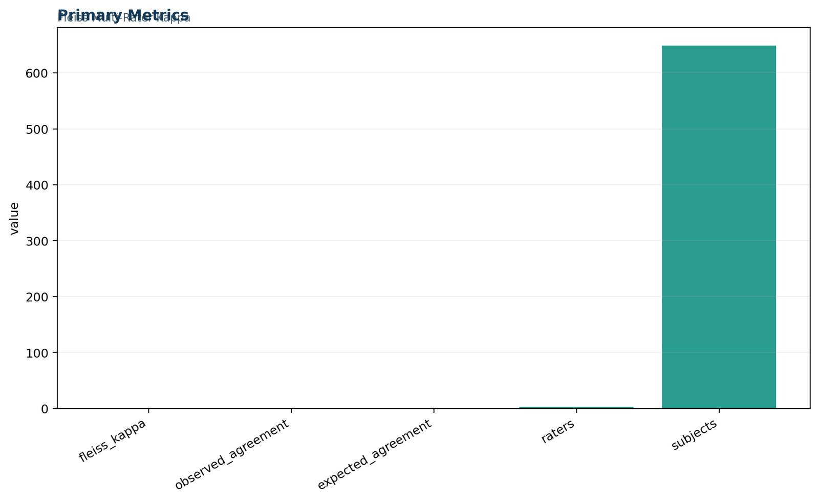
Python Chart 1: Primary Fleiss Kappa metrics
The primary panel places κ = 0.642126 beside observed agreement = 0.784284, expected agreement = 0.397228, three raters and 649 subjects. The subject count uses a much larger numerical scale than the coefficients, so the adjacent exact-value table should be used for precise comparison.
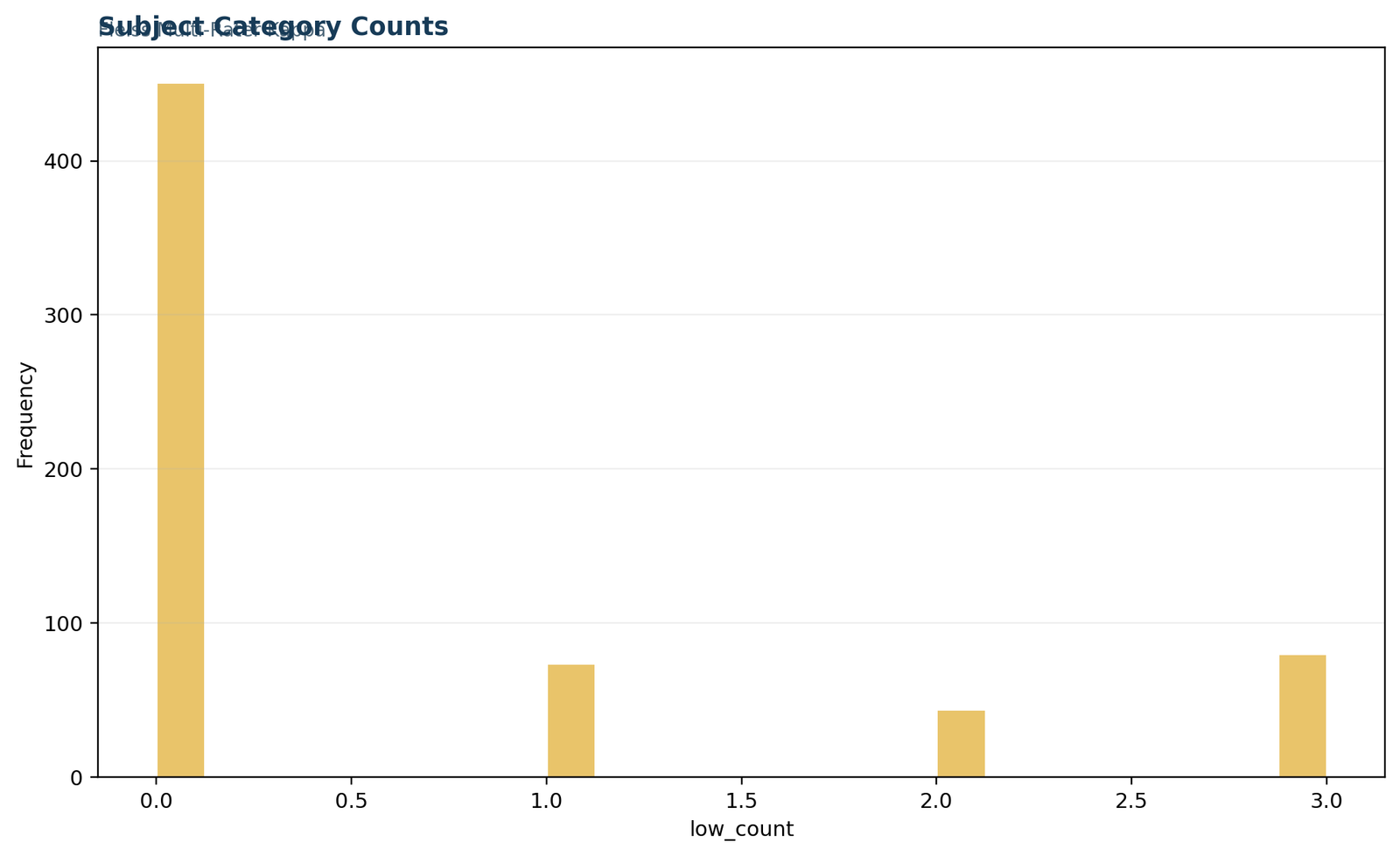
Python Chart 2: Subject category counts
The distribution of low-count values shows that 451 subjects were never classified low, 74 were low once, 44 were low twice and 80 were low on all three occasions. The same count matrix also contains the middle-count and high-count information used in the coefficient.
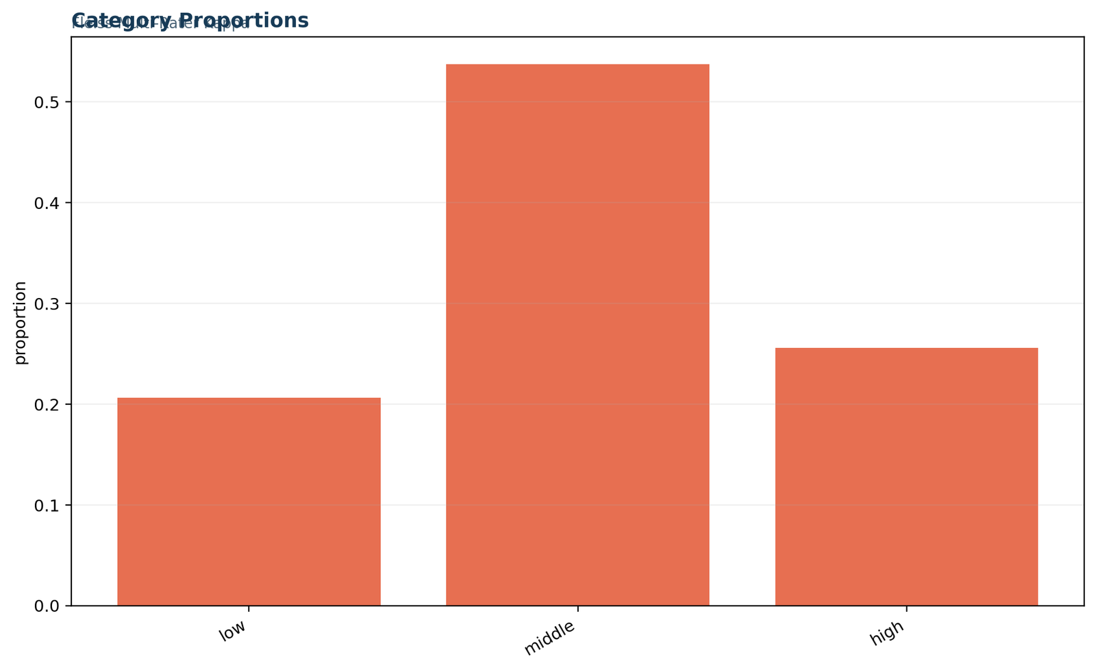
Python Chart 3: Pooled category proportions
The middle category accounts for 53.7750% of all ratings, compared with 20.6471% low and 25.5778% high. Squaring and summing these three proportions produces expected agreement of 0.397228.
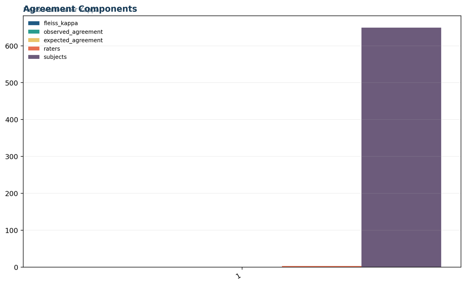
Python Chart 4: Agreement components
This component view presents the observed and expected terms beside the final coefficient and design counts. The exact calculation is κ = (0.784284 − 0.397228)/(1 − 0.397228).
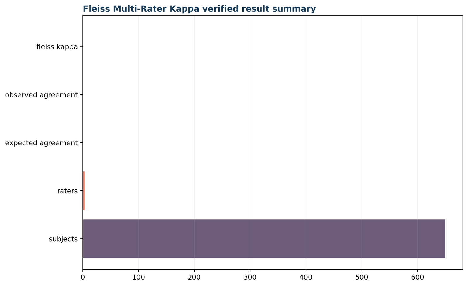
Python Chart 5: Verified result summary
The final verification panel records the coefficient, both agreement components, the three rating columns and the 649 complete subjects in one reproducibility summary.
What the Python charts establish
The first chart confirms the full numerical identity of the analysis. The second moves from a single coefficient back to the subject-level count structure. The third explains the chance baseline. The fourth links the components to the formula, and the fifth provides a compact audit record. Read together, they prevent the common mistake of reporting κ without explaining how category prevalence shaped the result.
The count matrix is the central Python object. Passing the raw G1, G2 and G3 values directly to a function that expects category counts would produce an invalid input. The matrix must contain one column per category rather than one column per rater. The categorical data in Python guide provides broader context for recoding and frequency validation.
Fleiss Kappa in R: package and manual verification
The R workflow reproduces the same values and visual evidence.
R workflow
library(irr)dat <- read.csv("dataset.csv")
ratings <- dat[c("G1", "G2", "G3")]
ratings <- na.omit(ratings)
band <- function(x) {
ifelse(x <= 9, 1L, ifelse(x <= 13, 2L, 3L))
}
ratings[] <- lapply(ratings, band)
# Package estimate from the subject-by-rater matrix
package_result <- kappam.fleiss(ratings, exact = FALSE, detail = TRUE)
print(package_result)
# Transparent manual verification
counts <- t(apply(ratings, 1, function(z) tabulate(z, nbins = 3)))
k <- ncol(ratings)
P_i <- (rowSums(counts^2) - k) / (k * (k - 1))
P_bar <- mean(P_i)
p_j <- colSums(counts) / sum(counts)
P_e <- sum(p_j^2)
kappa_manual <- (P_bar - P_e) / (1 - P_e)
cat("Subjects:", nrow(ratings), "\n")
cat("Ratings:", sum(counts), "\n")
cat("Category proportions:", p_j, "\n")
cat("Observed agreement:", P_bar, "\n")
cat("Expected agreement:", P_e, "\n")
cat("Fleiss Kappa:", kappa_manual, "\n")
The R package route receives a subject-by-rater matrix, while the manual route creates the count matrix internally. Keeping both routes in one script gives a direct cross-check of the package estimate.
Fleiss Kappa in R can be calculated directly from a data frame with subjects in rows and raters in columns. The verified R report recodes the grades identically, computes the coefficient and then reconstructs every component from a category-count matrix.
R Chart 1: Primary Fleiss Kappa metrics
The R verification reproduces the same coefficient and components: κ = 0.642126, observed agreement = 0.784284 and expected agreement = 0.397228 for 649 subjects and three rating columns.
R Chart 2: Subject category counts
The subject-count view verifies the distribution behind the low category. Most subjects never enter the low band, while 80 remain low across all three occasions.
R Chart 3: Pooled category proportions
The R margins match the Python and Excel margins exactly within floating-point precision. Middle is the dominant classification, which raises the expected-agreement baseline.
R Chart 4: Agreement components
The observed component exceeds the expected component by 0.387055. Dividing that excess by the available improvement of 0.602772 yields κ = 0.642126.
R Chart 5: Verified result summary
The final R panel records the same design counts and agreement statistics, demonstrating cross-software reproducibility rather than a software-specific result.
Package route
The package calculation is convenient for routine analysis. It expects the columns to represent the rating sources and the cell values to represent category codes. Category labels may be numeric or text, but their meaning must be consistent across columns.
The coefficient should be saved with the package version and all preprocessing rules. A reproducible script is preferable to manually copying a rounded output value.
Manual route
The manual verification tabulates the three ratings in each row, computes Pi, averages those values, derives pooled category proportions and applies the formula. This route exposes errors such as an incorrect number of categories, unequal row totals or a recoding mismatch.
See the categorical data in R guide for related factor and table operations.
Fleiss Kappa in SPSS: output and interpretation
SPSS confirms the case count, category coding and subject-level agreement pattern.
Fleiss Kappa in SPSS begins by recoding G1, G2 and G3 into the same three nominal categories. The supplied output uses 649 valid rows and creates low, middle and high counts for each subject before computing the subject-level agreement component.
SPSS descriptive verification
| Variable | Mean | SD | Minimum | Maximum |
|---|---|---|---|---|
| fk_low | 0.6194 | 1.05482 | 0 | 3 |
| fk_middle | 1.6133 | 1.26193 | 0 | 3 |
| fk_high | 0.7673 | 1.19662 | 0 | 3 |
| fk_subject_agreement | 0.7843 | 0.31213 | 0.33 | 1.00 |
SPSS frequency verification
The histogram therefore contains two bars: partial two-to-one agreement and complete three-to-zero agreement.
The SPSS crosstab confirms that all 649 subjects are valid for G1_cat3, G2_cat3 and G3_cat3. Its three-dimensional table reveals the exact direction of grade-band transitions. The pooled result is easier to understand when the crosstab is viewed beside the coefficient rather than after it has been collapsed into one number.
* Create the same three nominal categories used in Python, R, and Excel.
RECODE G1 G2 G3
(LOWEST THRU 9=1)
(10 THRU 13=2)
(14 THRU HIGHEST=3)
INTO G1_cat3 G2_cat3 G3_cat3.
VARIABLE LEVEL G1_cat3 G2_cat3 G3_cat3 (NOMINAL).
EXECUTE.* Native command in current SPSS versions.
FLEISS MULTIRATER KAPPA G1_cat3 G2_cat3 G3_cat3.
* Transparent subject-level agreement components used in the report.
COMPUTE fk_low=(G1_cat3=1)+(G2_cat3=1)+(G3_cat3=1).
COMPUTE fk_middle=(G1_cat3=2)+(G2_cat3=2)+(G3_cat3=2).
COMPUTE fk_high=(G1_cat3=3)+(G2_cat3=3)+(G3_cat3=3).
COMPUTE fk_subject_agreement=
(fk_low**2+fk_middle**2+fk_high**2-3)/6.
DESCRIPTIVES VARIABLES=fk_low fk_middle fk_high fk_subject_agreement
/STATISTICS=MEAN STDDEV MIN MAX.
FREQUENCIES VARIABLES=fk_subject_agreement
/STATISTICS=MEAN MEDIAN STDDEV /HISTOGRAM.
The categorical data in SPSS guide can help with value labels, recoding and crosstab checks. When using a native SPSS Fleiss command, retain the transparent manual component calculation as an audit because it shows how the coefficient relates to the exact data in the report.
SPSS workflow
* Create the same three nominal categories used in Python, R, and Excel.
RECODE G1 G2 G3
(LOWEST THRU 9=1)
(10 THRU 13=2)
(14 THRU HIGHEST=3)
INTO G1_cat3 G2_cat3 G3_cat3.
VARIABLE LEVEL G1_cat3 G2_cat3 G3_cat3 (NOMINAL).
EXECUTE.* Native command in current SPSS versions.
FLEISS MULTIRATER KAPPA G1_cat3 G2_cat3 G3_cat3.
* Transparent subject-level agreement components used in the report.
COMPUTE fk_low=(G1_cat3=1)+(G2_cat3=1)+(G3_cat3=1).
COMPUTE fk_middle=(G1_cat3=2)+(G2_cat3=2)+(G3_cat3=2).
COMPUTE fk_high=(G1_cat3=3)+(G2_cat3=3)+(G3_cat3=3).
COMPUTE fk_subject_agreement=
(fk_low**2+fk_middle**2+fk_high**2-3)/6.
DESCRIPTIVES VARIABLES=fk_low fk_middle fk_high fk_subject_agreement
/STATISTICS=MEAN STDDEV MIN MAX.
FREQUENCIES VARIABLES=fk_subject_agreement
/STATISTICS=MEAN MEDIAN STDDEV /HISTOGRAM.
The native command provides the coefficient in current SPSS versions. The transparent variables fk_low, fk_middle, fk_high and fk_subject_agreement reproduce the observed component and create useful diagnostics.
Fleiss Kappa in Excel: transparent workbook calculation
The workbook exposes every transform and formula instead of hiding the coefficient in one cell.
Fleiss Kappa in Excel is fully reproducible when each transformation is visible. The supplied workbook contains six organized sheets: Guide, Data_Input, Working, Calculations, Diagnostics and Reporting. This layout keeps the raw grades separate from formulas and prevents accidental overwriting of source values.
Guide and Data_Input
The Guide defines the analysis, category thresholds and interpretation. Data_Input stores G1, G2 and G3 for the 649 subjects. Source values should be pasted only into this sheet.
Working and Calculations
Working creates the three category codes, category counts and subject agreement. Calculations aggregates totals, proportions, P̄, Pe and the final coefficient.
Diagnostics and Reporting
Diagnostics checks row totals, pooled margins, complete cases and cross-software equality. Reporting presents the final values and a concise interpretation.
G1 class: =IF(Data_Input!A5<=9,1,IF(Data_Input!A5<=13,2,3))

Low count: =COUNTIF(A5:C5,1)

Middle count: =COUNTIF(A5:C5,2)

High count: =COUNTIF(A5:C5,3)

Subject agreement: =(SUMSQ(D5:F5)-3)/(3*(3-1))

Observed agreement: =AVERAGE(G5:G653)

Low proportion: =SUM(D5:D653)/(649*3)

Middle proportion: =SUM(E5:E653)/(649*3)

High proportion: =SUM(F5:F653)/(649*3)

Expected agreement: =SUMSQ(low_prop:high_prop)

Fleiss Kappa: =(observed_agreement-expected_agreement)/(1-expected_agreement)| Excel audit | Required result | Reason |
|---|---|---|
| Each category-code cell | 1, 2 or 3 | Prevents out-of-range labels |
| Each subject count row | Low + middle + high = 3 | Confirms a fixed number of ratings |
| Pooled category totals | 402 + 1,047 + 498 = 1,947 | Confirms complete counting |
| Pooled proportions | Sum = 1 | Confirms denominator and category coverage |
| Observed agreement | 0.7842835131 | Matches SPSS subject-level mean |
| Expected agreement | 0.3972284016 | Matches Python and R |
| Final coefficient | 0.6421256617 | Matches all verified workflows |
An Excel Fleiss Kappa calculator should use named cells for N, n, category totals, P̄ and Pe. It should also protect formula cells while leaving the input area editable. The workbook supplied with this article can be used as a transparent template for new datasets that have the same fixed-rater structure.
Excel workflow
G1 class: =IF(Data_Input!A5<=9,1,IF(Data_Input!A5<=13,2,3))

Low count: =COUNTIF(A5:C5,1)

Middle count: =COUNTIF(A5:C5,2)

High count: =COUNTIF(A5:C5,3)

Subject agreement: =(SUMSQ(D5:F5)-3)/(3*(3-1))

Observed agreement: =AVERAGE(G5:G653)

Low proportion: =SUM(D5:D653)/(649*3)

Middle proportion: =SUM(E5:E653)/(649*3)

High proportion: =SUM(F5:F653)/(649*3)

Expected agreement: =SUMSQ(low_prop:high_prop)

Fleiss Kappa: =(observed_agreement-expected_agreement)/(1-expected_agreement)
The Excel workbook stores the formulas in an auditable sequence. It is especially useful for teaching the calculation, checking a program’s result and documenting category boundaries for a report.
When results differ, compare the category totals first. If totals match, compare each subject’s count row. If those match, compare the expected-agreement formula. This sequence is faster and more reliable than changing software options at random.
Fleiss Kappa calculator and cross-software verification
Data shape and preprocessing must remain identical before results can be compared.
A reproducible Fleiss Kappa calculator must keep the data shape, category rules and chance model identical in every program. The raw 649 × 3 rating matrix is converted to a 649 × 3 subject-by-category count matrix. Each count row sums to three, pooled category totals sum to 1,947, and all programs must use the same formula for observed and expected agreement.
Fix categories
Use low ≤9, middle 10–13 and high ≥14 in every implementation.
Verify data shape
Rows are subjects; the three source columns are G1, G2 and G3.
Create counts
For each subject, count how many of the three ratings fall in each category.
Rebuild components
Calculate Pi, P̄, pooled pj, Pe and κ independently.
Compare outputs
Investigate any difference larger than ordinary display rounding.
Expected shape at each stage
| Stage | Rows | Columns | Row rule |
|---|---|---|---|
| Raw grade ratings | 649 | 3 | G1, G2 and G3 for one subject |
| Categorized ratings | 649 | 3 | Each cell is 1, 2 or 3 |
| Category-count matrix | 649 | 3 | Low + middle + high = 3 |
| Pooled category totals | 1 | 3 | 402 + 1,047 + 498 = 1,947 |
Exact cross-software targets
Fleiss Kappa versus Cohen Kappa, weighted kappa, ICC and percent agreement
Choose the coefficient that matches the number of raters, measurement scale and estimand.
The choice between Fleiss Kappa and another reliability statistic depends on the number of raters, whether categories are nominal or ordered, whether all subjects receive the same ratings, and whether exact identity or numerical closeness defines agreement.
| Method | Typical design | What counts as agreement | Use instead when |
|---|---|---|---|
| Fleiss Kappa | Multiple rating columns, common nominal categories | Exact category match, chance corrected | The current design has more than two rating columns and every mismatch is equally important |
| Cohen Kappa | Two raters or two methods | Exact or optionally weighted categorical agreement | Exactly two rating sources are the inferential target |
| Weighted multi-rater agreement | Multiple raters, ordered categories | Disagreements receive different penalties | Adjacent category errors are less serious than extreme errors |
| Intraclass correlation | Continuous or near-continuous ratings | Numerical similarity under a variance-components model | Distances between ratings are meaningful |
| Percent agreement | Any exact-match summary | Observed matches only | A simple descriptive rate is desired, but it should accompany—not replace—chance correction |
| Cross-tabulation and pairwise tables | Two categories or two rating columns at a time | Shows direction and location of disagreement | The analyst needs to diagnose which categories or pairs cause disagreement |
Fleiss Kappa versus Cohen Kappa
Cohen Kappa calculates expected agreement from the two raters’ separate marginal distributions. Fleiss Kappa uses pooled category proportions across all rating columns. With exactly two raters, the coefficients can therefore differ because the expected-agreement definitions are not identical.
Use Cohen’s formulation when two named raters are the design. Use Fleiss Kappa when a pooled multi-rater summary is intended. Do not call one a simple software replacement for the other.
Fleiss Kappa versus ICC
The intraclass correlation evaluates numeric ratings through between-subject and error variation. It can distinguish agreement from consistency depending on the model. Fleiss Kappa discards numeric distance after classification and asks only whether categories match.
Converting continuous scores to categories can simplify interpretation but loses information and makes results depend on cut points. Prefer the original numeric scale when the research question concerns numeric reliability.
Statistics such as Cramer’s V, the phi coefficient and the contingency coefficient describe association in contingency tables. They are not multi-rater agreement coefficients. A Pearson chi-square test assesses discrepancies from an independence model rather than chance-corrected exact agreement.
Fleiss Kappa diagnostics, limitations and common mistakes
Inspect prevalence, subject patterns and rater-specific distributions before trusting one number.
A trustworthy Fleiss Kappa interpretation includes diagnostics. The coefficient can be reduced by genuine inconsistency, highly uneven category prevalence, systematic marginal differences, ambiguous category definitions, missing ratings or simple data-shape mistakes.
Prevalence concentration
The middle category holds 53.775% of all ratings. This increases chance agreement to 0.3972. Always report pooled proportions so readers can see the baseline.
Rater or occasion drift
G3 has 194 high ratings versus 152 for both G1 and G2. The coefficient does not reveal this direction by itself. Compare each column’s distribution.
Pair-specific disagreement
G1 versus G3 has the lowest exact agreement at 75.19%, while G2 versus G3 has the highest at 82.28%. Pairwise tables identify where review is needed.
Category-boundary sensitivity
Moving a threshold by one score can reclassify many observations and alter every component. Perform sensitivity analyses only when alternative cut points are substantively defensible.
Missing ratings
A fixed three-rater formula cannot silently accept rows with two ratings. Document exclusions or use a method designed for varying rating counts.
Sampling uncertainty
The coefficient is an estimate. A confidence interval needs a stated method and should resample subjects, not individual cells.
Ten frequent errors
Sample size should be planned around the desired precision and the expected category distribution, not a universal minimum. More subjects usually improve precision, but rare categories, many raters and a target lower confidence bound all affect the requirement. A margin-of-error target is more informative than a fixed rule such as “30 subjects are enough.”
Finally, reliability is not validity. Raters can agree perfectly and still classify the wrong construct or use an unsuitable threshold system. Agreement analysis should be combined with content expertise and a validation plan.
How to report Fleiss Kappa in APA style
Report the design, category definitions, agreement components, coefficient and limitations.
A complete Fleiss Kappa report allows a reader to reconstruct what was classified, who or what provided the ratings, how categories were coded, how missing values were handled, and whether inference was performed.
Methods example
“Agreement in grade-band classification across G1, G2 and G3 was evaluated using unweighted Fleiss Kappa. Each score was classified as low (≤9), middle (10–13) or high (≥14). The analysis included 649 subjects with complete ratings on all three occasions. The coefficient was calculated from subject-level category counts and pooled category proportions.”
Results example
“Across 1,947 ratings, 20.65% were low, 53.78% were middle and 25.58% were high. Mean observed agreement was 0.784, and expected agreement from the pooled margins was 0.397. Fleiss Kappa was κ = 0.642. Complete agreement occurred for 439 of 649 subjects (67.64%); the remaining 210 subjects had a two-to-one split.”
Reporting checklist
Practice questions with answers
Why is 0.7843 not the final coefficient?
What would happen if the middle category became more dominant?
Why are pairwise percentages still reported?
Can the supplied output support a statement that p < .05?
When a significance test is later added, report the exact method and avoid interpreting a small p-value as proof of strong agreement. Statistical significance depends strongly on sample size, whereas the coefficient communicates magnitude. Also distinguish false-positive and false-negative risks using the principles of Type I and Type II error.
Fleiss Kappa PDF, Excel and software downloads
Open the exact Python, R and SPSS reports and the worked Excel workbook.
The four Fleiss Kappa downloads use the same 649 subjects, the same three category thresholds and the same unweighted coefficient. The PDF reports document software output, while the Excel workbook exposes the complete calculation.
R Fleiss Kappa ReportIndependent R calculation and matching numerical verification.Download R PDF
SPSS Fleiss Kappa OutputRecoding, descriptives, frequency table, histogram and crosstabs.Download SPSS PDF
Worked Excel AnalysisGuide, raw inputs, working formulas, calculations, diagnostics and report.Download Excel Workbook
Related statistical guides
Fleiss Kappa analysis references and verification trail
Every worked value is tied to a supplied report, workbook or component calculation.
The numerical claims in this article are tied to the supplied analysis artifacts rather than copied from a generic Fleiss Kappa example. The worked Excel workbook, SPSS output and independent Python and R reports use the same 649 subjects, the same three grade occasions and the same low–middle–high category boundaries.
Worked Excel audit
The workbook separates raw data, categorized working rows, final calculations, diagnostics and reporting. It documents the formula κ = (P̄ − Pe)/(1 − Pe) and reproduces κ = 0.6421256617 with no material difference from the verified reference.
SPSS audit
The SPSS output confirms 649 valid cases, three recoded categories and a mean subject-agreement value of 0.7843. Its frequency table contains 439 subjects with complete agreement and 210 subjects with one-versus-two partial agreement.
Python and R audit
The Python and R reports reproduce the same pooled category totals, category proportions, observed agreement, expected agreement and final coefficient. The chart sets provide a visual cross-check of every major component.
| Verified quantity | Value | Where it is checked |
|---|---|---|
| Subjects | 649 | Excel Guide and Calculations; SPSS case processing; Python and R summaries |
| Total ratings | 1,947 | Category totals and count-matrix row sums |
| Pooled category totals | 402, 1,047, 498 | Python/R category charts and Excel working columns |
| Mean observed agreement | 0.7842835131 | Excel formula, SPSS subject-agreement mean, Python and R |
| Expected agreement | 0.3972284016 | Squared pooled category proportions |
| Fleiss Kappa | 0.6421256617 | Excel, Python and R final result ledgers |
Fleiss Kappa FAQs
Answers to the design, formula, interpretation and software questions most often missed.
These Fleiss Kappa FAQs summarize the calculation and the decisions that matter most in applied work.
What is Fleiss Kappa?
How do you interpret Fleiss Kappa?
What is a good Fleiss Kappa value?
What is the Fleiss Kappa formula?
Can Fleiss Kappa be used for two raters?
Does Fleiss Kappa require the same raters for every subject?
Is Fleiss Kappa weighted?
Why can kappa be low when percent agreement is high?
Can Fleiss Kappa be negative?
How is Fleiss Kappa calculated in Python?
How is Fleiss Kappa calculated in R?
What was the result in this worked example?
Final conclusion
The three grade occasions showed agreement meaningfully above the pooled chance baseline. Observed agreement was 0.7843, expected agreement was 0.3972 and 439 of 649 subjects received the same grade-band classification on all three occasions. The result is reproducible in Python, R, SPSS and Excel.
Report the coefficient with the category margins and disagreement pattern. Do not claim a p-value or confidence interval that was not calculated, and do not describe the grade occasions as independent human raters. With those qualifications, the analysis provides a transparent and defensible summary of repeated categorical consistency.
Verified worked example
Related statistical guides
Continue with the agreement and reliability methods most closely connected to Fleiss Kappa.