
.mn-wrap{–ink:#172033;–muted:#607083;–navy:#123b5d;–blue:#176ea6;–teal:#087f6b;–amber:#b86b10;–rose:#a33a54;–line:#d8e3ea;–soft:#f5f9fc;–soft2:#eefbf8;–warn:#fff7e8;–danger:#fff1f2;–code:#101828;max-width:1120px;margin:0 auto;color:var(–ink);font-family:system-ui,-apple-system,BlinkMacSystemFont,”Segoe UI”,Arial,sans-serif;line-height:1.76}
.mn-wrap *{box-sizing:border-box}.mn-wrap h1,.mn-wrap h2,.mn-wrap h3,.mn-wrap h4{line-height:1.25}.mn-wrap h2{font-size:30px;color:var(–navy);margin:0 0 16px}.mn-wrap h3{font-size:23px;color:#245877;margin:28px 0 12px}.mn-wrap h4{font-size:18px;color:#263c52;margin:22px 0 9px}.mn-wrap p{margin:0 0 16px}.mn-wrap a{color:#0b6598;text-decoration:underline}.mn-wrap li{margin:7px 0}
.mn-hero{padding:36px;border:1px solid var(–line);border-radius:26px;background:linear-gradient(135deg,#eef7fb 0%,#fff 52%,#fff4e7 100%);box-shadow:0 14px 36px rgba(24,59,86,.08);margin:14px 0 26px}
.mn-kicker{display:inline-flex;align-items:center;gap:8px;padding:7px 13px;border-radius:999px;background:#e7f6f3;border:1px solid #bce5dc;color:#075f52;font-size:13px;font-weight:800;letter-spacing:.04em;text-transform:uppercase;margin-bottom:15px}
.mn-hero h1{font-size:43px;color:#102e46;margin:0 0 16px}.mn-hero p{font-size:20px;color:#2b3b4e;margin:0}.mn-badges{display:flex;flex-wrap:wrap;gap:10px;margin-top:22px}.mn-badge{padding:8px 12px;border-radius:999px;border:1px solid var(–line);background:#fff;font-weight:750;font-size:14px}
.mn-ad{padding:18px;border:1px dashed #aebbc8;border-radius:16px;text-align:center;color:#718096;background:#fcfdfe;margin:27px 0}.mn-ad span{display:block;font-size:11px;text-transform:uppercase;letter-spacing:.1em;margin-bottom:4px}
.mn-section{background:#fff;border:1px solid var(–line);border-radius:22px;padding:25px;margin:24px 0;box-shadow:0 8px 24px rgba(15,23,42,.035)}
.mn-note{background:#f5f9fd;border-left:5px solid var(–navy);border-radius:16px;padding:18px 20px;margin:19px 0}.mn-success{background:#ecfdf5;border:1px solid #bbf7d0;border-radius:17px;padding:18px 20px;margin:19px 0}.mn-warning{background:var(–warn);border:1px solid #f1d19b;border-radius:17px;padding:18px 20px;margin:19px 0}.mn-danger{background:var(–danger);border:1px solid #fecdd3;border-radius:17px;padding:18px 20px;margin:19px 0}
.mn-stat-grid{display:grid;grid-template-columns:repeat(4,minmax(0,1fr));gap:14px;margin:20px 0}.mn-stat{padding:17px;border:1px solid var(–line);border-radius:17px;background:var(–soft)}.mn-stat small{display:block;color:var(–muted);margin-bottom:6px}.mn-stat strong{display:block;font-size:23px;color:var(–navy)}
.mn-result-grid{display:grid;grid-template-columns:1fr 1fr;gap:18px;margin:20px 0}.mn-result{border:1px solid var(–line);border-radius:19px;padding:20px}.mn-result.method{background:#f1f8fc}.mn-result.meaning{background:#f0fbf7}.mn-result h3{margin:0 0 8px}.mn-result ul{margin:10px 0 0;padding-left:20px}
.mn-toc{columns:2;column-gap:34px;margin:0;padding-left:20px}.mn-toc li{break-inside:avoid;margin:8px 0}
.mn-problem-grid{display:grid;grid-template-columns:repeat(3,minmax(0,1fr));gap:15px}.mn-problem{border:1px solid var(–line);border-radius:18px;padding:18px;background:var(–soft)}.mn-problem strong{display:block;font-size:20px;color:var(–navy);margin-bottom:5px}.mn-problem span{color:var(–muted)}
.mn-flow{display:grid;grid-template-columns:1fr auto 1fr auto 1fr;gap:12px;align-items:stretch;margin:22px 0}.mn-step{border:1px solid var(–line);border-radius:18px;padding:19px;background:#fff}.mn-step b{display:block;color:var(–teal);font-size:13px;text-transform:uppercase;letter-spacing:.05em;margin-bottom:7px}.mn-arrow{display:flex;align-items:center;font-size:28px;color:#8aa0b2;font-weight:800}
.mn-formula{padding:18px;border:1px solid var(–line);border-radius:17px;text-align:center;background:#f7f9fc;font-weight:800;font-size:19px;color:var(–navy);margin:18px 0;overflow-x:auto}
.mn-table-wrap{overflow-x:auto;border:1px solid var(–line);border-radius:18px;margin:18px 0}.mn-table{width:100%;min-width:880px;border-collapse:collapse;background:#fff}.mn-table th{background:#edf5f9;color:#163d58;text-align:left;padding:12px;border-bottom:1px solid var(–line)}.mn-table td{padding:12px;border-bottom:1px solid #edf1f4;vertical-align:top}.mn-table tr:last-child td{border-bottom:none}
.mn-decision-grid{display:grid;grid-template-columns:repeat(2,minmax(0,1fr));gap:16px;margin:20px 0}.mn-decision{border:1px solid var(–line);border-radius:18px;padding:19px;background:#fff}.mn-decision h3{margin-top:0}.mn-decision.use{border-top:5px solid var(–teal)}.mn-decision.avoid{border-top:5px solid var(–amber)}
.mn-method-grid{display:grid;grid-template-columns:repeat(4,minmax(0,1fr));gap:13px;margin:20px 0}.mn-method{border:1px solid var(–line);border-radius:17px;padding:17px;background:#fff}.mn-method strong{display:block;color:var(–navy);font-size:18px;margin-bottom:7px}.mn-method p{font-size:14px;color:#405368;margin:0}
.mn-chart-story{border-top:1px solid var(–line);padding:30px 0 8px}.mn-chart-story:first-of-type{border-top:none;padding-top:4px}.mn-figure{margin:16px 0 18px;border:1px solid var(–line);border-radius:20px;overflow:hidden;background:#fff}.mn-figure img{display:block;width:100%;height:auto}.mn-figure figcaption{padding:13px 16px;background:#fbfdff;border-top:1px solid var(–line);color:var(–muted);font-size:14px}
.mn-insight-grid{display:grid;grid-template-columns:1fr 1fr;gap:13px}.mn-insight{border:1px solid var(–line);border-radius:16px;padding:16px;background:#fff}.mn-insight span{display:block;font-size:12px;font-weight:850;letter-spacing:.06em;text-transform:uppercase;color:var(–teal);margin-bottom:7px}.mn-insight p{margin:0}.mn-next{margin:13px 0 0;padding:13px 15px;border-radius:14px;background:#f3f7fb;color:#405368;font-size:14px}
.mn-metric-grid{display:grid;grid-template-columns:repeat(3,minmax(0,1fr));gap:14px}.mn-metric{border:1px solid var(–line);border-radius:17px;padding:17px;background:#fff}.mn-metric b{display:block;color:var(–navy);margin-bottom:6px}.mn-metric strong{font-size:20px;color:var(–teal)}
.mn-software-grid{display:grid;grid-template-columns:repeat(2,minmax(0,1fr));gap:16px}.mn-software{border:1px solid var(–line);border-radius:18px;padding:19px}.mn-software h3{margin:0 0 8px}.mn-software ul{padding-left:19px;margin:8px 0}
.mn-details details{border:1px solid var(–line);border-radius:15px;padding:14px 16px;margin:11px 0;background:#fff}.mn-details summary{cursor:pointer;font-weight:850;color:var(–navy)}.mn-details details>div{padding-top:13px}
.mn-code{background:var(–code);color:#e5e7eb;border-radius:17px;padding:17px;overflow-x:auto;font-size:13.5px;line-height:1.62}.mn-code code{font-family:Consolas,Monaco,”Courier New”,monospace}
.mn-two-col{display:grid;grid-template-columns:1fr 1fr;gap:18px}.mn-list-card{border:1px solid var(–line);border-radius:18px;padding:19px;background:#fff}.mn-list-card h3{margin:0 0 9px}.mn-list-card ul{padding-left:20px;margin:0}
.mn-apa-grid{display:grid;grid-template-columns:1fr 1fr;gap:16px;margin:18px 0}.mn-report{border:1px solid var(–line);border-radius:18px;padding:19px;background:#fff}.mn-report h3{margin:0 0 10px}.mn-copy{border-left:5px solid var(–teal);background:#f0fbf7;border-radius:15px;padding:17px 19px;margin:14px 0}.mn-copy p:last-child{margin-bottom:0}.mn-template{border:1px dashed #9fb0bf;border-radius:15px;background:#fbfdff;padding:16px;margin:12px 0}.mn-template code{white-space:normal;color:#20364a;font-family:inherit}
.mn-r-pair{margin:28px 0 34px;padding:20px;border:1px solid var(–line);border-radius:21px;background:#fbfdff}.mn-r-pair-title{margin:0 0 15px;font-size:17px;color:var(–navy);font-weight:850}.mn-r-chart-row{display:grid;grid-template-columns:repeat(2,minmax(0,1fr));gap:18px;align-items:start}.mn-r-chart-box{border:1px solid var(–line);border-radius:18px;overflow:hidden;background:#fff}.mn-r-chart-box figure{margin:0}.mn-r-chart-box img{display:block;width:100%;height:auto}.mn-r-chart-box figcaption{padding:12px 14px;background:#f7fafc;border-top:1px solid var(–line);color:var(–muted);font-size:13px}.mn-r-explanation-row{display:grid;grid-template-columns:repeat(2,minmax(0,1fr));gap:18px;margin-top:14px}.mn-r-explanation{border:1px solid var(–line);border-radius:17px;padding:17px;background:#fff}.mn-r-explanation h3{font-size:19px;margin:0 0 9px}.mn-r-label{display:block;font-size:12px;font-weight:850;letter-spacing:.06em;text-transform:uppercase;color:var(–teal);margin-bottom:6px}.mn-r-check{padding:11px 13px;border-radius:13px;background:#eef7fb;color:#405368;font-size:13px;margin-top:10px}
.mn-download-grid{display:grid;grid-template-columns:repeat(2,minmax(0,1fr));gap:14px}.mn-download{display:block;text-decoration:none!important;border:1px solid var(–line);border-radius:17px;padding:18px;background:#fff}.mn-download strong{display:block;color:var(–navy);font-size:18px;margin-bottom:5px}.mn-download span{color:var(–muted);font-size:14px}.mn-related{display:grid;grid-template-columns:repeat(2,minmax(0,1fr));gap:11px}.mn-related a{display:block;padding:12px 14px;border:1px solid var(–line);border-radius:14px;background:#f8fafc;text-decoration:none}.mn-faq details{border:1px solid var(–line);border-radius:15px;padding:15px 17px;margin:10px 0}.mn-faq summary{cursor:pointer;font-weight:850;color:var(–navy)}.mn-faq p{margin-top:11px}
html{scroll-behavior:smooth}.mn-top-anchor{position:absolute;top:0;left:0;width:1px;height:1px;overflow:hidden}.mn-back-to-top{position:fixed;right:22px;bottom:24px;width:48px;height:48px;display:flex;align-items:center;justify-content:center;border-radius:50%;background:var(–navy);color:#fff!important;text-decoration:none!important;font-size:25px;font-weight:900;box-shadow:0 10px 24px rgba(15,23,42,.24);z-index:9999;border:2px solid rgba(255,255,255,.85)}.mn-back-to-top:hover{background:var(–teal);transform:translateY(-3px)}.mn-back-to-top span{position:absolute;width:1px;height:1px;overflow:hidden;clip:rect(0,0,0,0)}
@media(max-width:900px){.mn-method-grid{grid-template-columns:repeat(2,1fr)}.mn-stat-grid,.mn-metric-grid{grid-template-columns:repeat(2,1fr)}.mn-result-grid,.mn-two-col,.mn-software-grid,.mn-download-grid,.mn-related,.mn-insight-grid,.mn-apa-grid,.mn-decision-grid,.mn-r-chart-row,.mn-r-explanation-row{grid-template-columns:1fr}.mn-flow{grid-template-columns:1fr}.mn-arrow{justify-content:center;transform:rotate(90deg)}.mn-toc{columns:1}.mn-problem-grid{grid-template-columns:1fr}.mn-hero h1{font-size:34px}}
@media(max-width:540px){.mn-stat-grid,.mn-metric-grid,.mn-method-grid{grid-template-columns:1fr}.mn-section,.mn-hero{padding:21px}.mn-hero h1{font-size:29px}.mn-hero p{font-size:17px}.mn-wrap h2{font-size:25px}.mn-back-to-top{right:15px;bottom:18px;width:44px;height:44px}}
/* Readable APA templates: deliberately avoid theme styling. */
.mn-template{
border:1px dashed #9fb0bf!important;
border-radius:15px!important;
background:#fbfdff!important;
padding:17px 19px!important;
margin:13px 0 20px!important;
color:#20364a!important;
box-shadow:none!important;
}
.mn-template,
.mn-template *{
color:#20364a!important;
background:transparent!important;
text-shadow:none!important;
box-shadow:none!important;
}
.mn-template-text{
display:block!important;
margin:0!important;
padding:0!important;
border:0!important;
font-family:system-ui,-apple-system,BlinkMacSystemFont,"Segoe UI",Arial,sans-serif!important;
font-size:16px!important;
font-weight:400!important;
line-height:1.78!important;
white-space:normal!important;
word-break:normal!important;
overflow-wrap:anywhere!important;
}
/* Final APA reporting cards */
.mn-apa-template-intro{
display:flex;
align-items:flex-start;
gap:12px;
padding:15px 17px;
margin:16px 0 18px;
border:1px solid #c9d9e5;
border-radius:15px;
background:#f5faff;
color:#29435a
}
.mn-apa-template-intro strong{color:var(--navy)}
.mn-apa-template-grid{
display:grid;
grid-template-columns:repeat(2,minmax(0,1fr));
gap:16px;
margin:16px 0 24px
}
.mn-apa-template-card{
border:1px solid var(--line);
border-radius:19px;
padding:19px;
background:#fff;
box-shadow:0 5px 16px rgba(15,23,42,.035)
}
.mn-apa-template-card.directional{grid-column:1/-1}
.mn-apa-template-head{
display:flex;
flex-wrap:wrap;
align-items:center;
gap:10px;
margin-bottom:13px
}
.mn-apa-template-head h4{
margin:0;
color:var(--navy);
font-size:20px
}
.mn-apa-status{
display:inline-flex;
align-items:center;
border-radius:999px;
padding:5px 10px;
font-size:12px;
line-height:1.2;
font-weight:850;
letter-spacing:.035em;
text-transform:uppercase
}
.mn-apa-status.ns{background:#eef4f8;color:#39556b;border:1px solid #cbd8e1}
.mn-apa-status.sig{background:#ecfdf5;color:#076451;border:1px solid #b7e8da}
.mn-apa-status.one{background:#fff7e8;color:#8a520a;border:1px solid #efcf98}
.mn-apa-template-copy{
border-left:5px solid var(--blue);
border-radius:14px;
background:#f8fbfe;
padding:16px 17px;
color:#20364a
}
.mn-apa-template-card.sig-card .mn-apa-template-copy{border-left-color:var(--teal)}
.mn-apa-template-card.directional .mn-apa-template-copy{border-left-color:var(--amber)}
.mn-apa-template-copy p{
margin:0 0 11px!important;
color:#20364a!important;
font-size:16px!important;
line-height:1.72!important
}
.mn-apa-template-copy p:last-child{margin-bottom:0!important}
.mn-slot{
display:inline-block;
border:1px solid #b9d2e3;
border-radius:7px;
background:#eaf5fc;
color:#164e72;
padding:1px 6px;
margin:1px 1px;
font-weight:750;
white-space:nowrap
}
.mn-apa-template-card.sig-card .mn-slot{
border-color:#b6dfd4;
background:#eaf9f5;
color:#086653
}
.mn-apa-template-card.directional .mn-slot{
border-color:#e3c68d;
background:#fff5df;
color:#87510b
}
.mn-template-tip{
display:block;
margin-top:11px;
color:var(--muted);
font-size:13px
}
/* Separate Python and R chart presentations */
.mn-cross-software{
padding:16px 18px;
border:1px solid #c8dfd8;
border-radius:16px;
background:#f0fbf7;
margin:16px 0 22px;
color:#284b43
}
.mn-chart-badge{
display:inline-flex;
margin-left:8px;
padding:4px 9px;
border-radius:999px;
border:1px solid #c8d8e3;
background:#f3f8fb;
color:#36566d;
font-size:11px;
font-weight:800;
letter-spacing:.035em;
text-transform:uppercase;
vertical-align:middle
}
@media(max-width:850px){
.mn-apa-template-grid{grid-template-columns:1fr}
.mn-apa-template-card.directional{grid-column:auto}
}
/* Final robust APA-template layout */
.mn-apa-template-grid{display:block!important;margin:16px 0 24px!important}
.mn-apa-template-card,.mn-apa-template-card.directional{
display:block!important;width:100%!important;grid-column:auto!important;
margin:0 0 18px!important;padding:20px!important;overflow:visible!important
}
.mn-apa-template-head{
display:flex!important;align-items:center!important;flex-wrap:wrap!important;
gap:10px!important;margin:0 0 13px!important
}
.mn-apa-template-head h4{margin:0!important;font-size:21px!important;line-height:1.3!important}
.mn-apa-template-copy{display:block!important;width:100%!important;padding:4px 17px!important}
.mn-template-row{
display:grid!important;grid-template-columns:118px minmax(0,1fr)!important;
gap:14px!important;align-items:start!important;padding:13px 0!important;
border-bottom:1px solid #dce7ee!important
}
.mn-template-row:last-child{border-bottom:0!important}
.mn-template-label{
display:block!important;color:#31566f!important;font-size:12px!important;
line-height:1.35!important;font-weight:800!important;letter-spacing:.055em!important;
text-transform:uppercase!important;padding-top:4px!important
}
.mn-template-row p{
display:block!important;margin:0!important;color:#20364a!important;
font-size:16px!important;line-height:1.75!important;min-width:0!important
}
.mn-field{
display:inline!important;padding:1px 4px!important;border-radius:4px!important;
background:#eaf5fc!important;color:#145274!important;font-weight:750!important;
box-decoration-break:clone;-webkit-box-decoration-break:clone
}
.mn-apa-template-card.sig-card .mn-field{background:#eaf9f5!important;color:#086653!important}
.mn-apa-template-card.directional .mn-field{background:#fff3d9!important;color:#81500c!important}
.mn-template-tip{
display:block!important;margin-top:12px!important;padding-top:11px!important;
border-top:1px dashed #cbd9e2!important;color:var(--muted)!important;font-size:13px!important
}
@media(max-width:650px){
.mn-template-row{grid-template-columns:1fr!important;gap:5px!important}
.mn-template-label{padding-top:0!important}
}
.mn-eqline{display:flex;flex-wrap:wrap;align-items:center;justify-content:center;gap:8px;padding:18px;border:1px solid var(--line);border-radius:17px;background:#f7f9fc;color:var(--navy);font-size:18px;font-weight:800;margin:17px 0;overflow-x:auto;text-align:center}
.mn-eqline .mn-frac{display:inline-grid;grid-template-rows:auto auto;text-align:center;vertical-align:middle;line-height:1.15}.mn-eqline .mn-frac span:first-child{border-bottom:1px solid currentColor;padding:0 5px 3px}.mn-eqline .mn-frac span:last-child{padding:3px 5px 0}
.mn-kpi-strip{display:grid;grid-template-columns:repeat(6,minmax(0,1fr));gap:11px;margin:18px 0}.mn-kpi{border:1px solid var(--line);border-radius:15px;padding:14px;background:#fff}.mn-kpi small{display:block;color:var(--muted);font-size:12px}.mn-kpi strong{display:block;color:var(--navy);font-size:19px;margin-top:4px}
.mn-mini-grid{display:grid;grid-template-columns:repeat(3,minmax(0,1fr));gap:14px}.mn-mini{border:1px solid var(--line);border-radius:16px;padding:16px;background:#fff}.mn-mini h4{margin:0 0 7px}.mn-mini p:last-child{margin-bottom:0}
.mn-wide-card{border:1px solid var(--line);border-radius:18px;padding:20px;background:#fff;margin:16px 0}.mn-wide-card h3{margin-top:0}
.mn-check-grid{display:grid;grid-template-columns:repeat(2,minmax(0,1fr));gap:14px}.mn-check-card{border:1px solid var(--line);border-radius:16px;padding:17px;background:#fff}.mn-check-card h3{margin:0 0 8px}.mn-check-card ul{margin:0;padding-left:20px}
.mn-fineprint{font-size:13px;color:var(--muted)}
@media(max-width:1000px){.mn-kpi-strip{grid-template-columns:repeat(3,1fr)}}
@media(max-width:720px){.mn-kpi-strip,.mn-mini-grid,.mn-check-grid{grid-template-columns:1fr}.mn-eqline{font-size:16px}}
McNemar’s Test: Formula, Interpretation, Calculator, Python, R, SPSS and Excel Guide
McNemar’s Test compares two correlated binary classifications recorded on the same people or matched pairs. This complete guide explains the null hypothesis, exact binomial method, uncorrected and continuity-corrected formulas, assumptions, calculator logic, effect estimates, APA reporting, Python and R visual evidence, SPSS and Excel workflows, and downloadable reports through a verified analysis of G2 and G3 pass status for 649 students.
649 complete pairs
67 discordant pairs
Exact p = 2.146 × 10⁻⁸
McNemar’s Test Model Overview
McNemar’s Test is a nonparametric test for paired nominal data with exactly two categories. It is designed for situations in which every observational unit contributes two linked binary outcomes: before versus after, method A versus method B, left side versus right side, matched case versus matched control, or two diagnostic classifications applied to the same participant.
The test does not ask whether the two variables are independent. It asks whether the two marginal proportions are equal, which is equivalent in a paired 2 × 2 table to asking whether the two types of disagreement occur with equal probability. For that reason, McNemar’s Test is often described as a test of marginal homogeneity or symmetry of discordant pairs.
What Question Does McNemar’s Test Answer?
In the worked analysis, the same 649 students have a G2 grade and a G3 grade. Each grade is converted to pass/fail status using the same threshold: a grade of 10 or higher is coded as pass. McNemar’s Test asks whether changing from G2 fail to G3 pass is as likely as changing from G2 pass to G3 fail.
Why Only the Discordant Pairs Determine the Test
The paired table contains two concordant cells on the diagonal and two discordant cells off the diagonal. Concordant pairs—fail/fail and pass/pass—describe stability or agreement, but they do not indicate a direction of change. Only the off-diagonal counts distinguish improvement from deterioration, so only those counts enter the McNemar statistic and exact binomial probability.
Worked Example at a Glance
The table contains 89 fail/fail students, 56 fail-to-pass students, 11 pass-to-fail students and 493 pass/pass students. The 67 discordant pairs are strongly unbalanced: 83.58% moved from fail to pass and 16.42% moved from pass to fail. The exact two-sided p-value is 2.145796 × 10⁻⁸. The continuity-corrected statistic is χ2(1) = 28.8955, with p = 7.638930 × 10⁻⁸.
When McNemar’s Test Is Not the Right Method
McNemar’s Test is not appropriate for two independent groups, for outcomes with three or more categories, for three or more repeated binary measurements, or when covariate adjustment is required. Independent groups require procedures such as the Chi-Square Test of Independence, while paired multi-category tables require McNemar–Bowker or Bowker symmetry methods. Three or more related binary measurements require Cochran’s Q Test.
Quick Answer: McNemar’s Test Result
The exact two-sided McNemar’s Test is the primary analysis because it treats the 67 discordant pairs as a binomial outcome under a 0.50 null probability. The continuity-corrected and uncorrected chi-square forms are reported as standard asymptotic comparisons.
Test Summary
- Procedure: two-sided exact McNemar’s Test
- Paired observations: 649
- Discordant total: 67
- Exact statistic: min(56, 11) = 11
- Decision at α = .05: reject H0
Substantive Meaning
- 56 students changed from fail to pass.
- 11 students changed from pass to fail.
- Net increase: 45 passes.
- Marginal increase: 45/649 = 6.93 percentage points.
- Discordant matched odds ratio: 56/11 = 5.09.
Table of Contents
- Research question, hypotheses and paired design
- When to use McNemar’s Test
- McNemar’s Test formula and manual calculation
- Variables and data dictionary
- Worked paired 2 × 2 table and complete results
- Assumptions and data requirements
- Exact, corrected, uncorrected and related tests
- McNemar’s Test calculator workflow
- Six Python chart interpretations
- Six R chart interpretations in paired rows
- Python, R, SPSS and Excel workflows
- Expandable software code
- Advanced interpretation and edge cases
- APA reporting for McNemar’s Test
- Common mistakes and corrections
- Analysis and reporting checklist
- Reports and worked Excel download
- Related Salar Cafe guides
- Frequently asked questions
- Conclusion
Research Question, Hypotheses and Paired Data Design
Research Question
Does the probability of changing from G2 fail to G3 pass equal the probability of changing from G2 pass to G3 fail for the same students?
Null and Alternative Hypotheses
| Hypothesis | Statistical statement | Meaning |
|---|---|---|
| Null hypothesis | H0: p01 = p10 | The two discordant transition probabilities are equal. |
| Two-sided alternative | H1: p01 ≠ p10 | Directional paired change is asymmetric. |
| Possible directional alternative | H1: p01 > p10 | Fail-to-pass transitions are more common; use only when prespecified. |
Why the Observations Are Paired
G2 and G3 belong to the same student. The two binary classifications are therefore correlated. An independent-proportions test would ignore the link and treat 649 first measurements and 649 second measurements as though they came from unrelated people. McNemar’s Test preserves the pair identifier and uses the transition table.
Methods Statement
Before running the test, define the two measurement occasions, the coding of the binary event, the direction of the rows and columns, and whether the alternative is two-sided or directional. Review Null and Alternative Hypotheses and Type I and Type II Error when planning the decision rule.
When to Use McNemar’s Test
Use McNemar’s Test When
- The outcome has exactly two categories.
- The same participants are classified twice.
- Pairs are created through explicit matching.
- The question concerns marginal change or directional discordance.
- Each complete pair contributes one first and one second classification.
- Pairs are independent of other pairs.
- A before/after, diagnostic-method or matched-case design is used.
- The analysis does not require covariate adjustment.
Choose Another Method When
- The two groups are independent rather than paired.
- The outcome has more than two categories.
- There are three or more repeated binary measurements.
- The response is continuous, count or ordinal rather than binary.
- Pairs are nested inside schools, clinics or households.
- Covariates, interactions or subject effects must be modeled.
- The main question is inter-rater agreement rather than marginal change.
- The data contain unpaired observations that cannot be reconciled.
Simple Test-Selection Logic
If no, use an independent-sample categorical procedure.
If yes, McNemar’s Test may be appropriate.
Use McNemar for two and Cochran’s Q for three or more.
Typical Applications
Before and after
Smoking status, treatment response, policy support or a yes/no symptom recorded before and after an intervention.
Two diagnostic methods
Positive/negative classifications from two tests applied to the same participants.
Matched pairs
Cases matched to controls, twins, paired body sites or deliberately matched experimental units.
McNemar’s Test Versus Independent-Proportion Procedures
A two-proportion z test, Fisher’s Exact Test and an ordinary Chi-Square Test of Independence assume independent groups. They are not substitutes for McNemar’s Test when both classifications belong to the same person or matched pair.
McNemar’s Test Versus Bowker’s Test
McNemar’s Test is the 2 × 2 form of a broader symmetry-testing idea. For a paired square table with three or more categories, McNemar–Bowker or Bowker’s Test of Symmetry compares all corresponding off-diagonal pairs.
McNemar’s Test Formula and Manual Calculation
Write the first binary classification in rows and the second classification in columns. Label the discordant off-diagonal counts b and c. The diagonal counts a and d are retained for descriptive reporting but do not enter the basic McNemar formulas.
| First measurement | Second = 0 | Second = 1 | Row total |
|---|---|---|---|
| First = 0 | a = concordant 0/0 | b = discordant 0→1 | a + b |
| First = 1 | c = discordant 1→0 | d = concordant 1/1 | c + d |
| Column total | a + c | b + d | N |
Step 1: Identify the Discordant Counts
Step 2: Exact Binomial McNemar’s Test
Under H0, each discordant pair has probability .50 of appearing in either direction. Conditional on the observed discordant total, the smaller off-diagonal count follows a binomial distribution.
The exact p-value can also be described as the probability, under a fair 50/50 discordant split, of observing an imbalance at least as extreme as 56 versus 11 in either direction.
Step 3: Uncorrected Asymptotic Statistic
With one degree of freedom, the uncorrected asymptotic p-value is 3.849404 × 10⁻⁸.
Step 4: Continuity-Corrected Statistic
The continuity-corrected p-value is 7.638930 × 10⁻⁸. It is larger than the uncorrected p-value because the correction reduces the statistic, but both forms reach the same substantive conclusion.
Step 5: Discordant Matched Odds Ratio
The approximate log-scale 95% confidence interval is 2.6673 to 9.7168. An exact conditional interval obtained by inverting the discordant binomial proportion is approximately 2.6390 to 10.7768. Always name the interval method because exact and asymptotic endpoints differ.
Step 6: Marginal Proportions and Paired Difference
The pass proportion increased by 6.93 percentage points. A normal-approximation 95% confidence interval for the paired marginal difference is approximately 4.52 to 9.35 percentage points. This magnitude estimate complements the hypothesis test.
Variables and Data Dictionary
| Variable | Role | Coding | N | Meaning in the analysis |
|---|---|---|---|---|
| G2 | Original first grade | Grade from 0 to 19 | 649 | Source variable for the first binary status. |
| G3 | Original second grade | Grade from 0 to 19 | 649 | Source variable for the second binary status. |
| G2 pass | First paired binary classification | 0 if G2 < 10; 1 if G2 ≥ 10 | 649 | Row variable in the paired table. |
| G3 pass | Second paired binary classification | 0 if G3 < 10; 1 if G3 ≥ 10 | 649 | Column variable in the paired table. |
| Pair identifier | Linking field | One unique record per student | 649 | Ensures the two classifications remain paired. |
Observed Paired 2 × 2 Table
| G2 pass status | G3 fail (0) | G3 pass (1) | Row total |
|---|---|---|---|
| G2 fail (0) | 89 | 56 | 145 |
| G2 pass (1) | 11 | 493 | 504 |
| Column total | 100 | 549 | 649 |
Transition Categories
| Transition | Count | Share of all pairs | Role |
|---|---|---|---|
| Fail → fail | 89 | 13.71% | Concordant; descriptive only. |
| Fail → pass | 56 | 8.63% | Discordant count b. |
| Pass → fail | 11 | 1.69% | Discordant count c. |
| Pass → pass | 493 | 75.96% | Concordant; descriptive only. |
Worked Paired 2 × 2 Table and Complete Results
Primary Inferential Results
| Method | Statistic | Reference distribution | P-value | Decision at α = .05 |
|---|---|---|---|---|
| Exact McNemar’s Test | min(b,c) = 11 | Binomial(67, .50) | 2.145796 × 10⁻⁸ | Reject H0 |
| Continuity-corrected McNemar | χ2 = 28.895522 | χ2(1) | 7.638930 × 10⁻⁸ | Reject H0 |
| Uncorrected McNemar | χ2 = 30.223881 | χ2(1) | 3.849404 × 10⁻⁸ | Reject H0 |
Magnitude and Descriptive Results
| Measure | Estimate | 95% interval | Interpretation |
|---|---|---|---|
| G2 pass proportion | 0.776579 | — | 504 of 649 students passed at G2. |
| G3 pass proportion | 0.845917 | — | 549 of 649 students passed at G3. |
| Paired marginal difference, G3 − G2 | 0.069337 | Approx. [0.04520, 0.09347] | Pass status increased by 6.93 percentage points. |
| Discordant matched odds ratio, b/c | 5.090909 | Approx. [2.6673, 9.7168] | Fail-to-pass changes were about five times as common. |
| Discordant upward probability | 56/67 = 0.835821 | Exact [0.72520, 0.91509] | Among changers, 83.58% moved upward. |
| Concordance proportion | 582/649 = 0.896764 | — | Most classifications were unchanged. |
Statistical Interpretation
The exact two-sided p-value is much smaller than .05, .01 and .001. The null hypothesis of equal discordant transition probabilities is rejected. The evidence is not merely a threshold crossing; the observed discordant split is 56 versus 11, far from the 33.5 versus 33.5 balance expected under H0.
Practical Interpretation
The G3 pass rate is 6.93 percentage points higher than the G2 pass rate. Among the 67 students whose status changed, a fail-to-pass transition was approximately 5.09 times as frequent as a pass-to-fail transition. This expresses both the overall margin change and the direction within discordant pairs.
Agreement Versus Change
Overall concordance is high at 89.68%, largely because 493 students passed at both occasions. High agreement does not contradict the significant McNemar result. Agreement summarizes how many pairs match; McNemar’s Test examines whether the mismatches are directionally balanced. For a direct agreement analysis, use Cohen’s Kappa alongside the transition table rather than replacing McNemar’s Test.
McNemar’s Test Assumptions and Data Requirements
McNemar’s Test has fewer distributional assumptions than a parametric paired test, but it still depends on the design, coding and independence structure. The test should not be described as assumption-free.
| Assumption or requirement | What it means | Worked example status |
|---|---|---|
| Paired observations | Each row contains two linked classifications from the same participant or matched pair. | Met: G2 and G3 belong to the same student. |
| Binary outcome at both occasions | Each classification has exactly two mutually exclusive categories. | Met: fail versus pass using threshold 10. |
| Same category definition | The meaning of 0 and 1 is consistent across the two measurements. | Met: the same pass threshold is used. |
| Independence between pairs | One participant’s pair should not determine another participant’s pair. | Assumed for the 649 students. |
| Complete pairing | The 2 × 2 table should be based on pairs with both classifications observed. | Met in the worked workbook: N = 649 complete pairs. |
| Prespecified alternative | Two-sided or directional testing should be chosen before examining the split. | Two-sided is used as the primary analysis. |
| Adequate discordant count for approximation | The chi-square version needs enough discordant pairs; exact inference avoids this approximation. | 67 discordant pairs support both exact and asymptotic comparisons. |
What Does Not Need to Be Assumed?
McNemar’s Test does not require normally distributed measurements, equal variances, a continuous outcome, or equal numbers in the two binary categories. It does require valid pairing and binary coding.
Why the Number of Discordant Pairs Matters
The effective information for the test is b + c, not the full N. A study may contain thousands of concordant pairs but very few discordant pairs. In that situation, the exact binomial version is more defensible than relying on the chi-square approximation.
Missing Data
A participant missing G2 or G3 cannot be placed in the paired transition table. Excluding incomplete pairs is complete-pair analysis and can be biased if missingness is related to outcome change. Report how many pairs were excluded and consider a model-based strategy when missingness is substantial.
Exact, Corrected, Uncorrected and Related-Test Comparisons
Uses Binomial(b+c, .50) for the discordant split.
Uses a one-unit continuity correction in the chi-square statistic.
Uses the asymptotic chi-square formula without continuity correction.
Reduces exact-test conservatism but is not the ordinary exact p-value.
Numerical Comparison
| Method | Statistic or tail | P-value | When emphasized |
|---|---|---|---|
| Exact two-sided McNemar | 11 in the smaller discordant direction | 2.1458 × 10⁻⁸ | Primary finite-sample result. |
| Continuity-corrected chi-square | 28.8955 | 7.6389 × 10⁻⁸ | Common conservative asymptotic form. |
| Uncorrected chi-square | 30.2239 | 3.8494 × 10⁻⁸ | Large-discordance approximation. |
McNemar’s Test Versus Chi-Square Independence
The ordinary chi-square test of independence evaluates association between two categorical variables measured on independent observations. McNemar’s Test evaluates marginal change within pairs. Applying an independence test to the current transition table ignores the repeated-measure link and answers a different question.
McNemar’s Test Versus Fisher’s Exact Test
Fisher’s Exact Test is an exact procedure for an independent 2 × 2 table with conditioned margins. It does not preserve the paired transition structure. The exact McNemar procedure is also based on an exact distribution, but it conditions on the total number of discordant pairs and evaluates their directional split.
McNemar’s Test Versus Paired t Test or Wilcoxon Signed-Rank Test
A paired t test compares the mean of a quantitative paired difference; the Wilcoxon signed-rank test evaluates a paired ordinal or continuous shift. McNemar’s Test is the corresponding binary paired procedure. Converting a rich quantitative variable to pass/fail may answer a useful threshold question but loses information about the size of grade changes.
McNemar’s Test Versus Agreement Measures
Cohen’s Kappa estimates agreement beyond chance. McNemar’s Test evaluates marginal asymmetry. A table can show high kappa and a significant McNemar result, or low kappa and a nonsignificant McNemar result, because the statistics target different properties.
McNemar’s Test Versus Cochran’s Q
McNemar’s Test compares two related binary conditions. Cochran’s Q Test extends the same repeated-binary logic to three or more conditions or time points. A significant Cochran’s Q result is often followed by pairwise McNemar comparisons with multiplicity adjustment.
McNemar’s Test Versus Bowker Symmetry
McNemar’s Test is appropriate when each paired classification has two categories. Bowker’s symmetry test handles paired square tables with three or more categories by comparing each off-diagonal cell with its reflected counterpart.
McNemar’s Test Calculator: Step-by-Step Workflow
A reliable McNemar’s Test calculator must accept a paired 2 × 2 transition table and identify the two discordant cells. A calculator that treats all four cells as independent frequencies is not performing the paired test.
Calculator Inputs for the Worked Example
| Input | Value | Meaning |
|---|---|---|
| First fail, second fail | 89 | Concordant negative pairs. |
| First fail, second pass | 56 | Discordant upward transitions, b. |
| First pass, second fail | 11 | Discordant downward transitions, c. |
| First pass, second pass | 493 | Concordant positive pairs. |
| Alternative | Two-sided | Either transition direction can be more common. |
| Primary method | Exact binomial | Finite-sample two-sided p-value. |
| Alpha | 0.05 | Prespecified decision threshold. |
Calculator Step 1: Confirm the Table Orientation
Rows represent G2 and columns represent G3. Reversing the two occasions leaves the exact two-sided p-value unchanged but reverses the direction of the matched odds ratio and the wording of improvement versus deterioration.
Calculator Step 2: Confirm the Discordant Cells
The calculator should identify 56 and 11 as b and c. The diagonal counts 89 and 493 must not enter the test statistic. They remain important for overall sample description and agreement reporting.
Calculator Step 3: Choose Exact or Asymptotic Inference
Select the exact binomial result when the discordant total is small, when an exact finite-sample result is desired, or when the analysis plan specifies it. With 67 discordant pairs, both exact and chi-square versions are stable and provide useful cross-checks.
Calculator Step 4: Verify the Formulas
Calculator Step 5: Report Proportions and Direction
The G2 pass proportion is 77.66%, the G3 pass proportion is 84.59%, and the paired increase is 6.93 percentage points. Report these quantities with the transition counts and p-value. “Significant” alone does not tell the reader what changed.
How to Find the Proportion from McNemar’s Test
McNemar’s Test itself is based on discordant counts, but several proportions are useful: the first marginal proportion, the second marginal proportion, the proportion of all pairs that are discordant, and the proportion of discordant pairs moving in the focal direction. For this example, 56/67 = 83.58% of changers moved from fail to pass.
Six Python McNemar’s Test Chart Interpretations
The Python workflow contains six dedicated figures: the paired transition table, discordant counts, null distribution, two-sided rejection region, method comparison and result summary. Each Python asset supplied for this post is displayed in this section.
Chart 1: Paired G2-by-G3 Transition Table Python
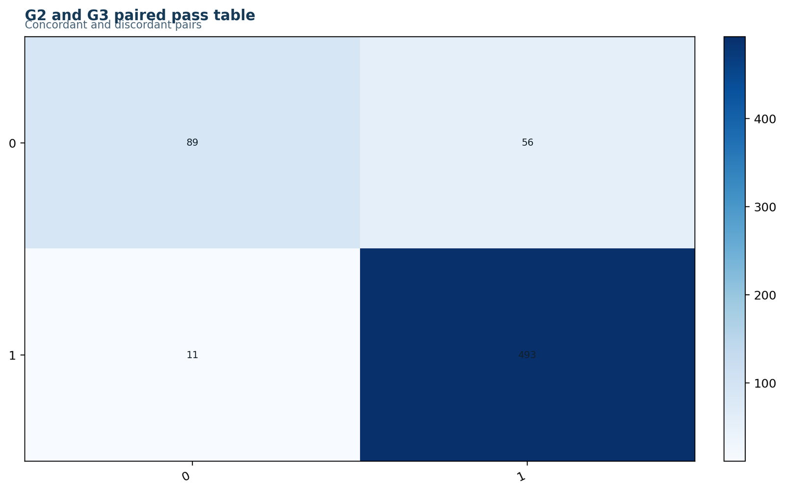
The diagonal contains 582 concordant pairs, while the off-diagonal contains 67 discordant pairs.
Fail/fail = 89, fail/pass = 56, pass/fail = 11, pass/pass = 493.
Most students remain in the same status, but the relatively few changes are strongly directional.
The table preserves pairing and prevents an incorrect independent-samples analysis.
Chart 2: Discordant Transition Counts Python
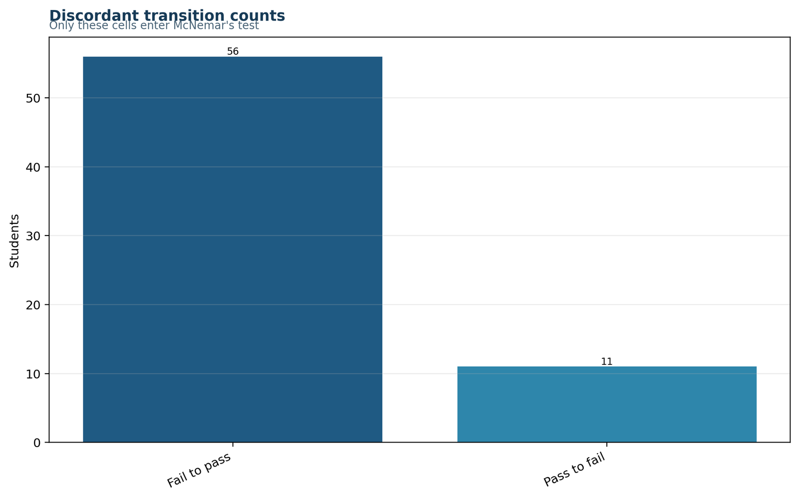
Fail-to-pass transitions greatly exceed pass-to-fail transitions.
b = 56, c = 11, b + c = 67, b/c = 5.09.
Among changers, 83.58% move upward and 16.42% move downward.
The null hypothesis expects the discordant total to split equally between the two directions.
Chart 3: Exact Null Distribution Python
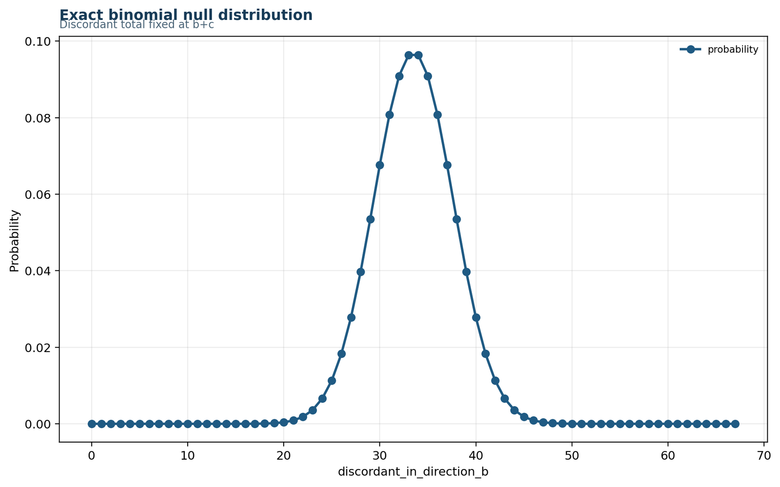
The observed smaller count of 11 lies far into the lower tail of the null distribution.
X ~ Binomial(67, .50); observed X = 11.
A balanced discordant split would normally produce counts near the center, not 11 versus 56.
The exact reference distribution requires no large-sample chi-square approximation.
Chart 4: Two-Sided Exact Rejection Region Python
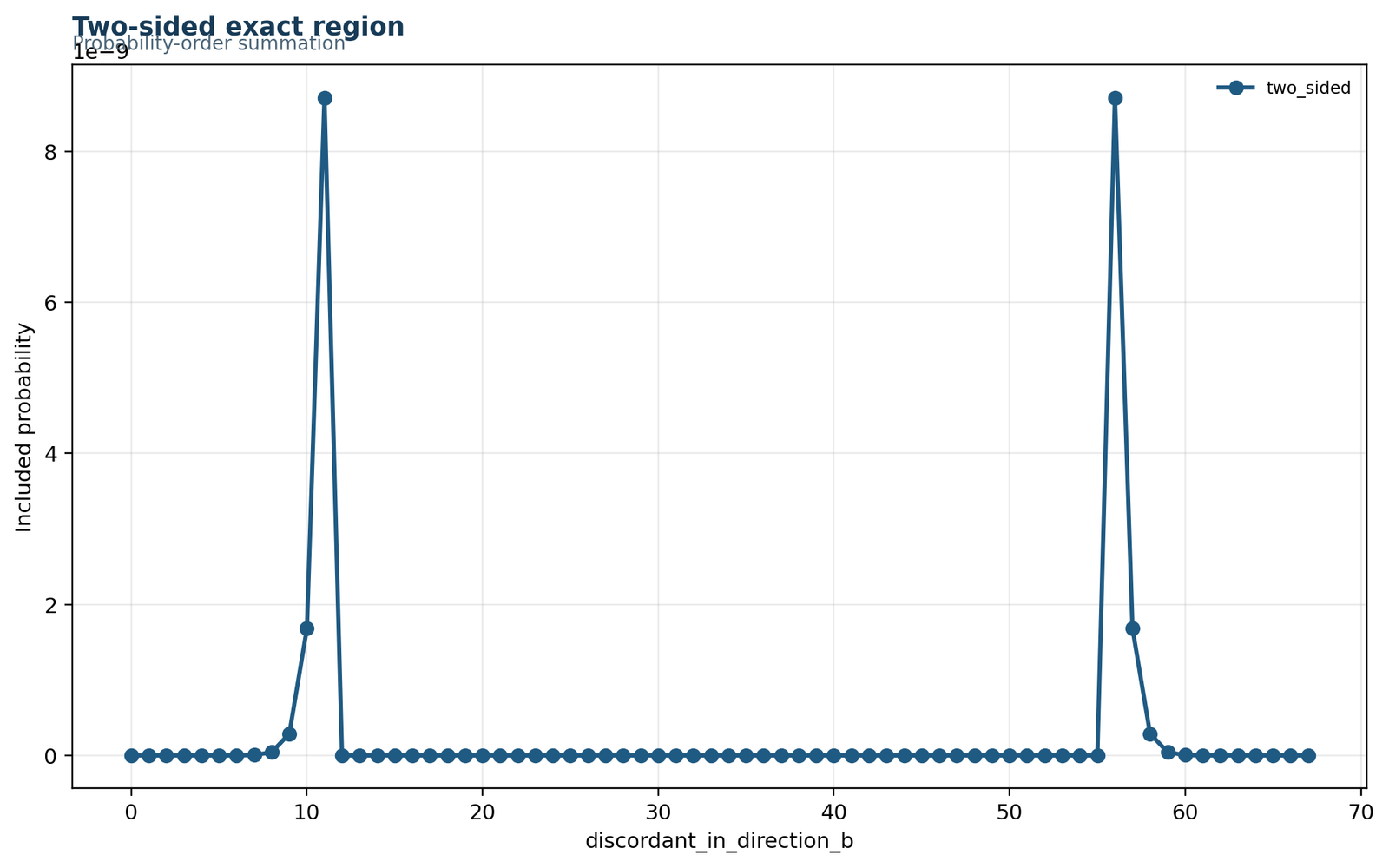
The observed lower-tail count is mirrored by an equally extreme upper-tail region.
Two-sided p = 2 × P(X ≤ 11) = 2.145796 × 10⁻⁸.
The two-sided alternative protects against selecting the direction only after seeing the data.
One-sided and two-sided p-values answer different prespecified hypotheses.
Chart 5: Exact and Chi-Square Method Comparison Python
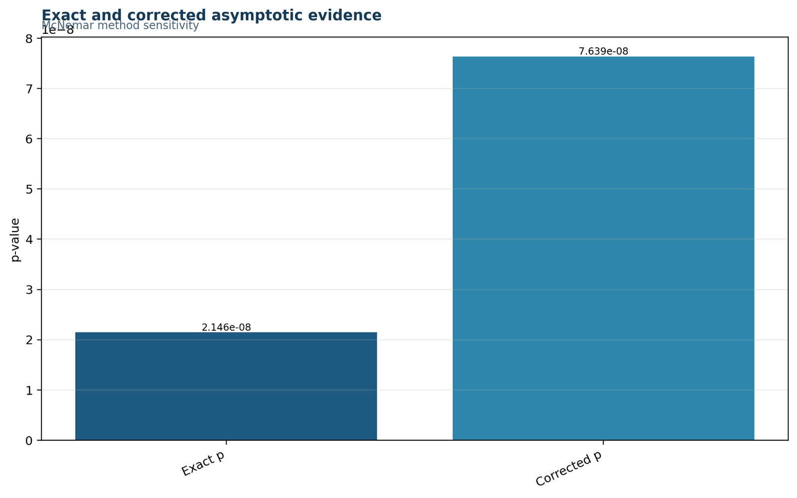
All accepted McNemar variants return extremely small p-values.
Exact = 2.15e−8; corrected = 7.64e−8; uncorrected = 3.85e−8.
The continuity correction is more conservative, but it does not change the decision.
Method choice is transparent and the conclusion is robust rather than dependent on one implementation.
Chart 6: McNemar’s Test Result Summary Python
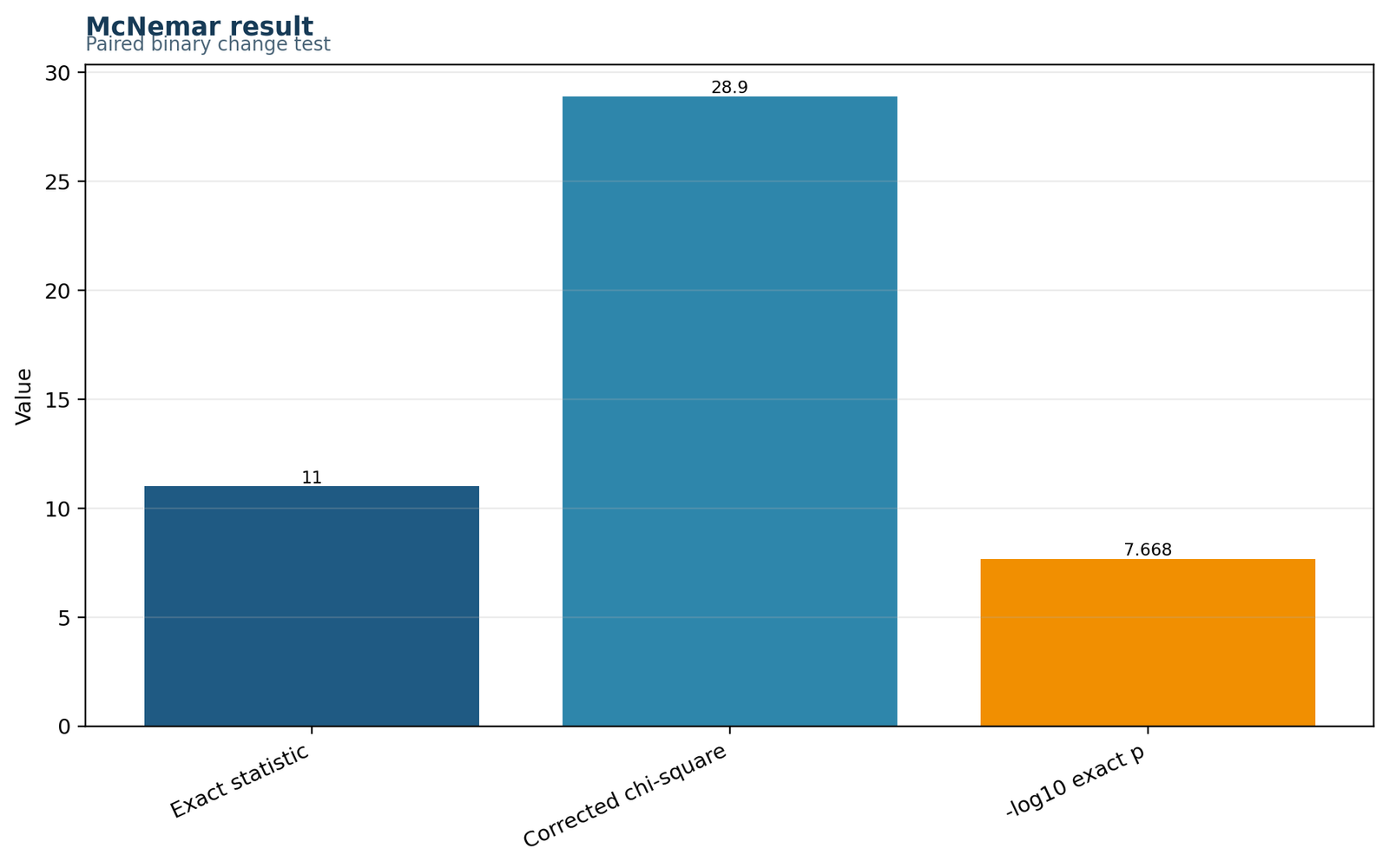
The final panel combines the 56-to-11 split with the exact and asymptotic results.
Net increase = 45; paired margin change = +6.93 percentage points.
The inferential rejection corresponds to a visible and interpretable direction of change.
The panel discourages reporting a p-value without counts and effect estimates.
R McNemar’s Test Results: All Six R Charts
This section follows the uploaded sample post format and displays every R chart as a separate figure. None is shared with, merged into, or omitted because of the Python section.
R Chart 1: Paired Table
R Chart 2: Discordant Counts
The complete paired table contains 649 matched records. The concordant cells total 582 and the discordant cells total 67.
McNemar’s Test uses the directional imbalance between 56 and 11. The discordant-pair odds ratio is 56/11 = 5.0909.
R Chart 3: Exact Null Distribution
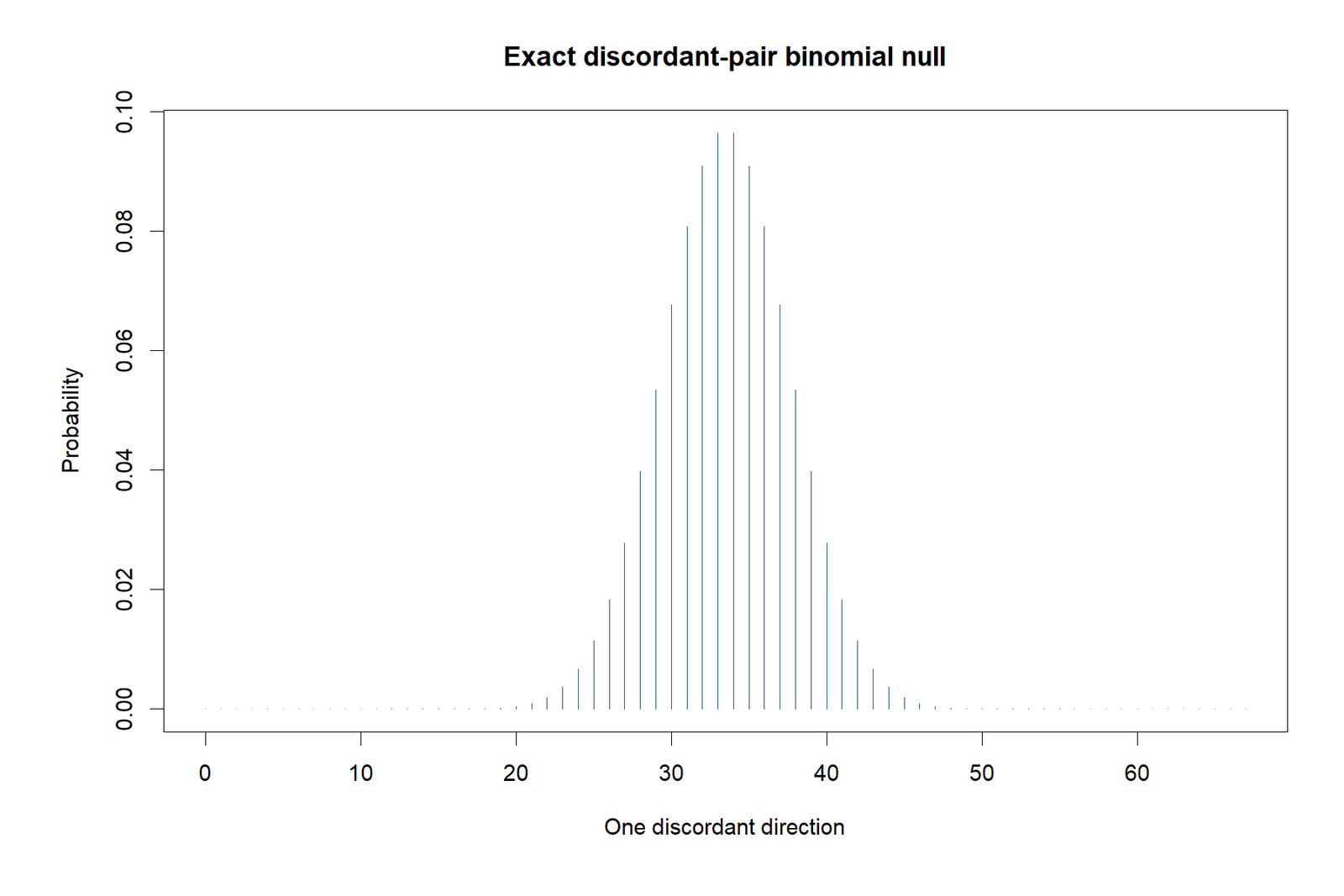
R Chart 4: Concordant and Discordant Pairs
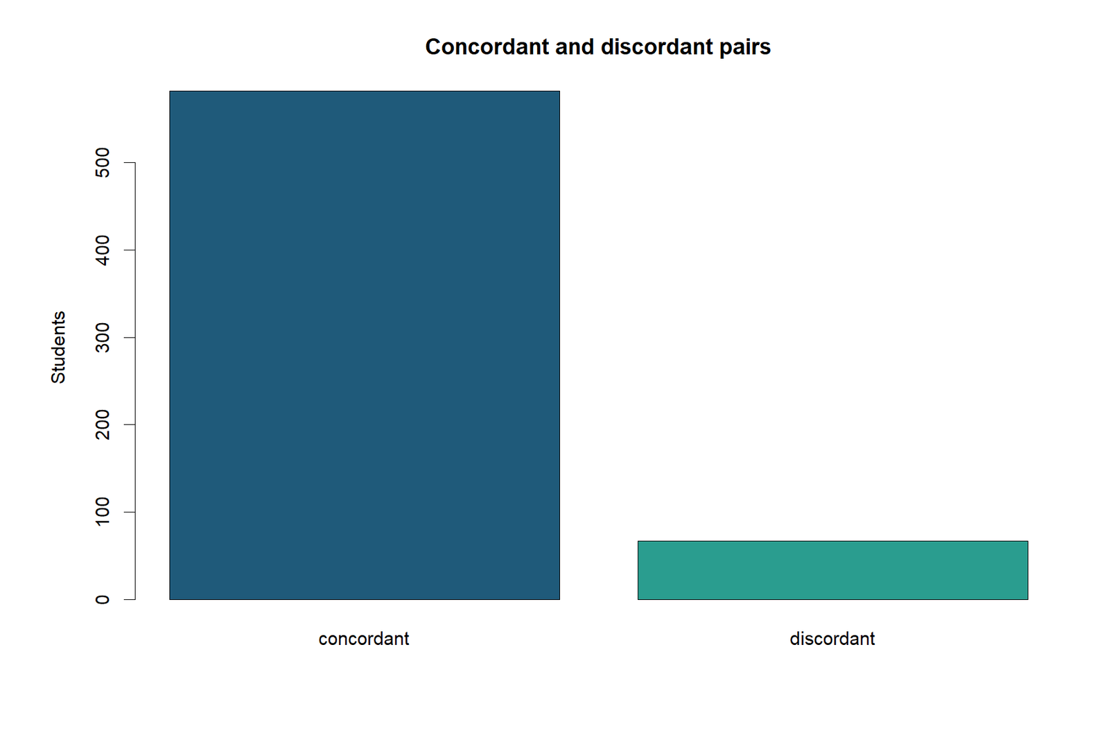
Under marginal homogeneity, the two directions are equally likely among discordant pairs. The exact two-sided p-value is 2.145796 × 10⁻⁸.
Concordant pairs describe stability, while the asymmetry within the 67 discordant pairs determines the McNemar result.
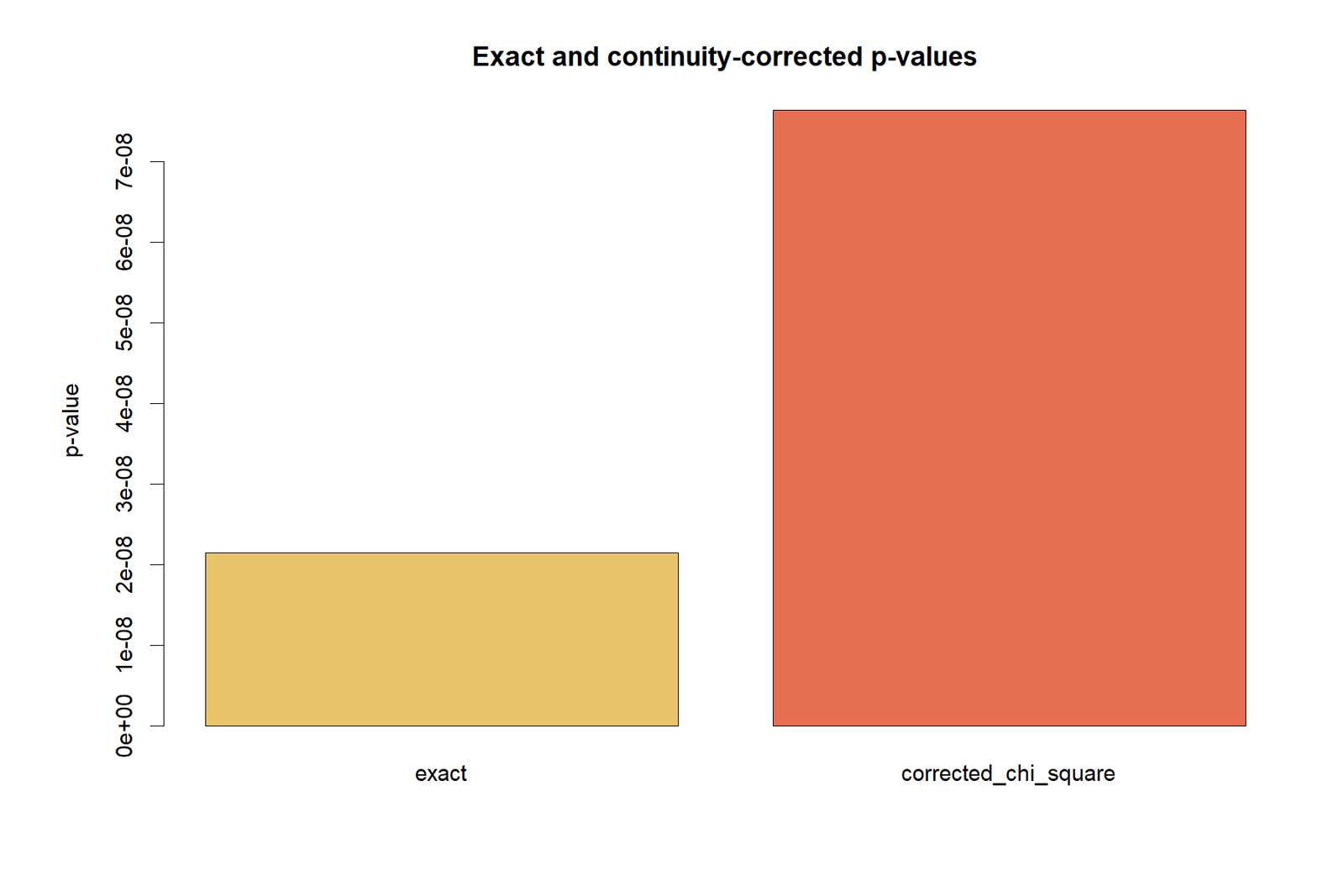
R Chart 5: Exact and Asymptotic Results
R Chart 6: Result Summary
All reported procedures reject marginal homogeneity. The continuity-corrected statistic is χ²(1) = 28.8955, with p < .001.
The post-period pass rate is higher by 6.93 percentage points, with substantially more fail-to-pass than pass-to-fail transitions.
McNemar’s Test in Python, R, SPSS and Excel
McNemar’s Test in Python
Python can build the paired crosstab, run an exact McNemar procedure and calculate comparison statistics. Keep one row per participant so pairing is never lost.
- Create binary G2 and G3 pass variables.
- Build the transition table in the intended row/column order.
- Run the exact version as the primary analysis.
- Run corrected and uncorrected versions for comparison.
- Calculate marginal proportions, paired difference and b/c.
Worked target: table [[89, 56], [11, 493]], exact statistic 11 and p = 2.145796 × 10⁻⁸.
McNemar’s Test in R
Base R provides mcnemar.test() for the chi-square form. The exact p-value can be obtained directly from the discordant counts with binom.test().
- Build a 2 × 2 table with identical category order.
- Use
correct = TRUEfor continuity correction. - Use
correct = FALSEfor the uncorrected statistic. - Use
binom.test(b, b+c, p=.5)for exact inference. - Report row and column direction.
McNemar’s Test in SPSS
SPSS can run McNemar’s Test for paired dichotomous variables through the legacy nonparametric tests workflow or equivalent syntax. The data should remain in wide paired form: one row per participant and one binary variable for each occasion.
- Verify that both variables use the same 0/1 coding.
- Request frequencies or a crosstab to verify the four cells.
- Run McNemar on the paired variable list.
- Check whether the output reports exact or asymptotic significance.
- Export the output and report transition counts separately.
McNemar’s Test in Excel
Excel can reproduce the full paired table, exact p-value, corrected and uncorrected statistics, margins and effect estimates with transparent formulas.
- Use
COUNTIFSto calculate the four transitions. - Use
BINOM.DISTfor the exact two-sided tail. - Use
CHISQ.DIST.RTfor the asymptotic p-values. - Calculate b/c and (b−c)/N.
- Audit formulas against Python, R or SPSS.
Software Agreement in the Worked Analysis
| Output | Python | R | SPSS | Excel |
|---|---|---|---|---|
| Paired table | 89, 56, 11, 493 | Same | Same after coding check | Same via COUNTIFS |
| Exact p-value | 2.145796e−8 | 2.145796e−8 | Verify requested exact output | 2.145796e−8 |
| Corrected χ² | 28.895522 | 28.895522 | Expected standard output | 28.895522 |
| Direction | 56 > 11 | 56 > 11 | Same after table orientation | 56 > 11 |
Expandable McNemar’s Test Code
The code is collapsed by default so the public article remains readable. Expand only the software block you need.
Python code for exact, corrected and uncorrected McNemar’s Test
import numpy as np
from scipy.stats import binomtest, chi2
from statsmodels.stats.contingency_tables import mcnemar

# Rows: G2 fail, G2 pass
# Columns: G3 fail, G3 pass
table = np.array([[89, 56],
                  [11, 493]])

b = int(table[0, 1])
c = int(table[1, 0])
n = int(table.sum())

exact = mcnemar(table, exact=True)
corrected = mcnemar(table, exact=False, correction=True)
uncorrected = mcnemar(table, exact=False, correction=False)

# Independent verification of the exact two-sided tail
exact_check = binomtest(b, b + c, p=0.5, alternative="two-sided")

p_g2 = (table[1, 0] + table[1, 1]) / n
p_g3 = (table[0, 1] + table[1, 1]) / n
paired_difference = (b - c) / n
matched_or = b / c

print(table)
print(exact.statistic, exact.pvalue)
print(corrected.statistic, corrected.pvalue)
print(uncorrected.statistic, uncorrected.pvalue)
print(exact_check.pvalue)
print(p_g2, p_g3, paired_difference, matched_or)
R code for exact and chi-square McNemar’s Test
tab <- matrix(
  c(89, 56,
    11, 493),
  nrow = 2,
  byrow = TRUE,
  dimnames = list(
    G2 = c("Fail", "Pass"),
    G3 = c("Fail", "Pass")
  )
)

b <- tab["Fail", "Pass"]
c <- tab["Pass", "Fail"]
N <- sum(tab)

exact_result <- binom.test(
  x = b,
  n = b + c,
  p = 0.5,
  alternative = "two.sided"
)

corrected_result <- mcnemar.test(tab, correct = TRUE)
uncorrected_result <- mcnemar.test(tab, correct = FALSE)

p_g2 <- sum(tab["Pass", ]) / N
p_g3 <- sum(tab[, "Pass"]) / N
paired_difference <- (b - c) / N
matched_or <- b / c

tab
exact_result
corrected_result
uncorrected_result
c(p_g2 = p_g2,
  p_g3 = p_g3,
  paired_difference = paired_difference,
  matched_or = matched_or)
SPSS syntax outline
* G2_pass and G3_pass must be coded 0/1 for the same cases.
FREQUENCIES VARIABLES=G2_pass G3_pass.
CROSSTABS
  /TABLES=G2_pass BY G3_pass
  /CELLS=COUNT ROW COLUMN TOTAL.

NPAR TESTS
  /MCNEMAR=G2_pass WITH G3_pass (PAIRED)
  /MISSING ANALYSIS.
Excel formula layout
Assume G2 pass is in column B and G3 pass is in column D.

B5  =COUNTIFS(Data_Input!B:B,0,Data_Input!D:D,0)   // a = 89
B6  =COUNTIFS(Data_Input!B:B,0,Data_Input!D:D,1)   // b = 56
B7  =COUNTIFS(Data_Input!B:B,1,Data_Input!D:D,0)   // c = 11
B8  =COUNTIFS(Data_Input!B:B,1,Data_Input!D:D,1)   // d = 493

B10 =B6+B7                                           // discordant total
B11 =MIN(B6,B7)                                      // exact statistic
B12 =MIN(1,2*BINOM.DIST(B11,B10,0.5,TRUE))           // exact p
B13 =(B6-B7)^2/B10                                   // uncorrected chi-square
B14 =CHISQ.DIST.RT(B13,1)                            // uncorrected p
B15 =(ABS(B6-B7)-1)^2/B10                            // corrected chi-square
B16 =CHISQ.DIST.RT(B15,1)                            // corrected p
B17 =B6/B7                                           // matched odds ratio
B18 =(B6-B7)/SUM(B5:B8) // paired margin differenceAdvanced McNemar’s Test Topics
Exact Versus Asymptotic Inference
The exact version uses the conditional binomial distribution of one discordant direction given b + c. The asymptotic version replaces that finite distribution with a χ2(1) approximation. A common rule of thumb recommends exact inference when b + c is small, but the exact test remains valid for larger totals. The main trade-off is discreteness and potential conservatism.
Continuity Correction
The correction subtracts one from |b−c| before squaring. It usually increases the p-value relative to the uncorrected statistic. Software defaults differ, so a report should say “continuity corrected” when that form is used.
Mid-p McNemar Variant
A mid-p calculation subtracts half the probability of the observed outcome from the ordinary exact tail. It often has better average power but is not a fully conservative exact test. Do not label a mid-p result as the ordinary exact McNemar p-value.
One-Sided McNemar’s Test
A directional alternative can test whether b is greater than c or vice versa. The direction must be specified before examining the transition counts. Choosing one-sided inference after seeing that 56 exceeds 11 inflates the Type I error rate.
Zero Discordant Counts
If b + c = 0, all pairs are concordant and the data contain no information about directional change. The exact p-value is 1 by convention, and b/c is undefined. If one discordant cell is zero and the other is positive, the exact test remains possible but the raw matched odds ratio is infinite or zero; report an exact interval or a carefully justified continuity adjustment.
Matched Odds Ratio
The ratio b/c is the natural odds ratio for the direction of discordance. It is not the same as an ordinary cross-sectional odds ratio calculated from row and column totals. For the current table, 56/11 = 5.09.
Confidence Interval for the Paired Difference
McNemar’s Test supplies a hypothesis test, not automatically a confidence interval for the marginal difference. Several paired-binomial interval methods exist. Name the method and keep its assumptions separate from the exact p-value. Here, the paired difference is +0.0693 with an approximate interval of +0.0452 to +0.0935.
Thresholding a Quantitative Outcome
G2 and G3 are quantitative grades, but this analysis converts them to pass/fail. The binary question is useful when the threshold has substantive meaning. It should not replace an analysis of the original grade change when the amount of change also matters.
Clustered or Repeated Pairs
McNemar’s Test assumes independence between pairs. Repeated observations within schools, families, clinics or subjects can require conditional logistic regression, generalized estimating equations or mixed-effects logistic models.
Covariate Adjustment
McNemar’s Test is unadjusted. When the goal is to estimate a paired effect while controlling for additional variables, use a model designed for correlated binary outcomes rather than stratifying repeatedly and creating many small tests.
Power and Sample Size
Power depends primarily on the expected discordant proportion and how unequal the two discordant directions are. A large total N does not guarantee power if nearly every pair is concordant. Planning should specify expected p01, p10, alpha, power and anticipated incomplete-pair rate.
Multiple Pairwise McNemar Tests
After a significant Cochran’s Q test, pairwise McNemar comparisons can identify which conditions differ. Adjust the family of p-values with a prespecified multiplicity method such as Holm’s procedure rather than interpreting every comparison at an unadjusted .05 level.
APA Reporting for McNemar’s Test
A complete report identifies the paired design, binary coding, discordant counts, version of the test, statistic when applicable, p-value, direction and a magnitude estimate. Avoid reporting only “McNemar’s Test was significant.”
Worked Exact APA Statement
An exact two-sided McNemar’s Test compared paired G2 and G3 pass status among 649 students. Fifty-six students changed from fail to pass, whereas 11 changed from pass to fail. The discordant transition probabilities differed significantly, exact p = 2.15 × 10⁻⁸. The G3 pass proportion was 6.93 percentage points higher than the G2 pass proportion, and the discordant matched odds ratio was 5.09.
Continuity-Corrected APA Statement
A continuity-corrected McNemar’s Test indicated that G2 and G3 pass-status margins differed significantly, χ2(1, N = 649) = 28.90, p < .001. More students changed from fail to pass (56) than from pass to fail (11), corresponding to a net increase of 45 passes.
Reusable Reporting Templates
Exact significant result
Significant
An exact two-sided McNemar’s Test compared first binary measure with second binary measure for N complete pairs.
b count pairs changed from 0 to 1, whereas c count changed from 1 to 0.
The discordant transition probabilities differed significantly, exact p = p-value.
The paired marginal difference was difference, and the matched odds ratio was b/c.
Use the exact label only when the exact binomial version was actually run.
Nonsignificant result
Not significant
McNemar’s Test compared first binary measure and second binary measure for N pairs.
The discordant counts were b and c.
The data did not provide sufficient evidence of unequal transition probabilities, test/statistic, p = p-value.
The confidence interval and observed direction should be reported; failure to reject does not prove identical margins.
Prespecified directional result
One-sided
A one-sided exact McNemar’s Test evaluated whether 0→1 transitions were more frequent than 1→0 transitions.
The observed discordant counts were b and c.
The prespecified directional hypothesis was supported/not supported, one-sided exact p = p-value.
Do not convert a two-sided result to one-sided after inspecting the direction.
What to Include in a Methods Section
Pass status was coded as 1 for grades of 10 or higher and 0 otherwise. G2 and G3 status were paired within student. McNemar’s Test evaluated equality of the two discordant transition probabilities. The exact two-sided binomial result was primary, and the continuity-corrected chi-square result was used as a sensitivity check.
P-Value Formatting
For ordinary APA reporting, a result this small can be written as p < .001. Because the exact numerical output is useful in a technical worked example, the guide also reports 2.15 × 10⁻⁸. Do not write p = .000.
Common McNemar’s Test Mistakes and How to Correct Them
| Mistake | Why it is wrong | Correction |
|---|---|---|
| Using an ordinary chi-square independence test | It ignores within-pair correlation. | Use the paired transition table and McNemar’s Test. |
| Including diagonal counts in the statistic | Only b and c provide directional information. | Use b + c in the denominator and b − c in the numerator. |
| Calling the test an agreement test | Marginal symmetry is not the same as agreement. | Report kappa separately when agreement is the target. |
| Using McNemar for three or more categories | The 2 × 2 formula does not cover larger square tables. | Use Bowker’s symmetry test. |
| Using McNemar for three or more occasions | The method compares only two related binary measures. | Use Cochran’s Q, followed by adjusted pairwise tests if needed. |
| Reporting only a p-value | Direction and practical magnitude remain hidden. | Report b, c, marginal proportions, difference and matched OR. |
| Ignoring table orientation | The sign and odds-ratio direction can reverse. | State which variable is in rows and which is in columns. |
| Choosing one-sided after viewing counts | This inflates false-positive risk. | Prespecify direction or retain the two-sided test. |
| Using the chi-square form with very few discordant pairs | The asymptotic approximation can be poor. | Use the exact binomial version. |
| Dropping incomplete pairs without reporting them | Missingness can alter the transition pattern. | Report exclusions and consider sensitivity analysis. |
| Interpreting significance causally | The test establishes asymmetry, not why it occurred. | Use design and subject knowledge for causal claims. |
McNemar’s Test Analysis and Reporting Checklist
Design
- Same participants or valid matched pairs.
- Exactly two binary classifications.
- Pairs independent of other pairs.
- Measurement order defined.
Data
- Same category coding at both occasions.
- Complete-pair count reported.
- Four transition cells verified.
- Missing pairs documented.
Inference
- b and c identified correctly.
- Two-sided or directional alternative prespecified.
- Exact or asymptotic version named.
- Software options verified.
Reporting
- Both discordant counts reported.
- Marginal proportions and difference reported.
- Matched odds ratio or directional share reported.
- Agreement and change kept conceptually separate.
McNemar’s Test Reports and Worked Excel Download
Use the files below to review the verified calculations, software output and formula-driven workbook.
Download R PDF ReportR calculations, exact-binomial verification and all six supplied R figures.
Download SPSS PDF OutputSPSS paired analysis and output evidence.
Download Worked Excel AnalysisInput data, paired table, formulas, diagnostics and reporting sheet.
Frequently Asked Questions About McNemar’s Test
What is McNemar’s Test used for?
McNemar’s Test is used to compare two paired binary classifications and determine whether the two discordant transition probabilities are equal.
What is the null hypothesis for McNemar’s Test?
The null hypothesis states that the probability of changing from category 0 to category 1 equals the probability of changing from category 1 to category 0.
Which cells are used in McNemar’s Test?
Only the two off-diagonal discordant cells b and c determine the test statistic and p-value. The diagonal cells describe concordance.
How do I find the McNemar test statistic?
For the uncorrected form, calculate (b−c)2/(b+c). For the continuity-corrected form, calculate (|b−c|−1)2/(b+c). For the exact form, the statistic is often reported as min(b,c).
How do I find proportions from a McNemar table?
The first and second marginal proportions are calculated from their row and column totals divided by N. The directional discordant proportion is b/(b+c), and the paired marginal difference is (b−c)/N.
When should the exact McNemar test be used?
The exact version is especially useful when b+c is small or when finite-sample exact inference is required. It is also valid for larger discordant totals.
What is the difference between McNemar’s Test and chi-square?
McNemar’s Test is for paired binary data. The ordinary chi-square test of independence assumes independent observations and does not account for pairing.
What is the difference between McNemar’s Test and Fisher’s Exact Test?
Fisher’s Exact Test analyzes independent 2 × 2 tables. Exact McNemar inference analyzes the two directions of discordance within pairs.
What is the difference between McNemar’s Test and Bowker’s Test?
McNemar’s Test is for paired 2 × 2 tables. Bowker’s Test extends symmetry testing to paired square tables with three or more categories.
What is the difference between McNemar’s Test and Cochran’s Q?
McNemar’s Test compares two related binary measurements. Cochran’s Q compares three or more related binary measurements.
Does a significant McNemar result mean poor agreement?
No. A table can have high agreement and still show significant marginal asymmetry when the disagreements mainly point in one direction.
Can McNemar’s Test be one-sided?
Yes, when a directional hypothesis is specified before examining the data. Post-hoc conversion from two-sided to one-sided is not appropriate.
What if b or c is zero?
The exact test can still be calculated when one discordant cell is zero, but the raw b/c odds ratio becomes zero or infinite. Use an exact interval and report counts clearly.
How is the current result interpreted?
Fail-to-pass transitions occurred much more frequently than pass-to-fail transitions. The exact p-value is approximately 2.15 × 10⁻⁸, the pass margin increased by 6.93 percentage points, and the matched odds ratio is 5.09.
McNemar’s Test Conclusion
McNemar’s Test is the correct procedure when the same participants or matched pairs contribute two binary classifications and the research question concerns directional marginal change. It preserves the pairing and bases inference on the two off-diagonal discordant counts.
In the worked G2-to-G3 example, 56 students changed from fail to pass and 11 changed from pass to fail. The exact two-sided p-value was 2.145796 × 10⁻⁸. The continuity-corrected statistic was χ2(1) = 28.895522, p = 7.638930 × 10⁻⁸, and the uncorrected statistic was χ2(1) = 30.223881, p = 3.849404 × 10⁻⁸.
The substantive conclusion is clear: pass status improved more often than it deteriorated. The pass margin increased by 6.93 percentage points, and the discordant matched odds ratio was 5.09. A complete report therefore includes the four transition counts, both marginal proportions, the exact-test specification, direction, effect estimates and a careful noncausal interpretation.

