
Likelihood Ratio Chi Square: Formula, Interpretation, Python, R, SPSS, SAS and Excel Guide
Likelihood Ratio Chi Square tests whether two categorical variables are associated by comparing the maximized likelihood of an independence model with the likelihood of a saturated model. This complete guide explains the hypotheses, formula, expected counts, cell contributions, residuals, Pearson comparison, effect size, software workflows, charts, APA reporting and downloadable results through a worked 2 × 4 analysis of school and G3 grade band for 649 students.
649 observations
G² = 57.0752
df = 3, p = 2.48 × 10⁻¹²
Likelihood Ratio Chi Square Model Overview
Likelihood Ratio Chi Square, also called the likelihood-ratio chi-square statistic, deviance chi-square or G-squared test for a contingency table, evaluates whether a model of categorical independence fits the observed cell counts. The method is closely related to the chi-square test of independence, but it measures discrepancy with log-likelihood rather than Pearson squared residuals.
What question does it answer?
The worked example asks whether school membership—GP or MS—is independent of a four-category G3 grade band. Under independence, the grade-band profile should be the same in the two schools apart from ordinary sampling variation. A significant Likelihood Ratio Chi Square result means the observed 2 × 4 table is too different from the expected independence table to be explained plausibly by chance alone.
How the likelihood-ratio statistic is built
The independence model produces an expected count for every cell from the row and column margins. The statistic then compares each observed count with its expected count using the term 2O ln(O/E). Cells that fit the model closely contribute little. Cells with large observed-to-expected discrepancies contribute strongly to the total. For a broader foundation, review cross-tabulation, frequency and relative frequency tables and two-way tables and relative frequency.
Worked example at a glance
The observed table contains 423 GP students and 226 MS students. Grade-band totals are 100, 355, 148 and 46. The independence model expects GP counts of 65.18, 231.38, 96.46 and 29.98, and MS counts of 34.82, 123.62, 51.54 and 16.02. The verified Likelihood Ratio Chi Square result is G²(3) = 57.0752, p = 2.4766 × 10⁻¹², with Cramér’s V = 0.2966.
What the result means substantively
MS has many more students than expected in grade band 1, while GP has substantially fewer. GP has more students than expected in grade bands 2, 3 and 4, while MS has fewer. The association is therefore not just a mathematical rejection: the two schools have meaningfully different grade-band profiles.
Quick Answer: Likelihood Ratio Chi Square Result
The primary analysis is a two-way Likelihood Ratio Chi Square test of independence for school and four G3 grade bands.
Test summary
- Procedure: Likelihood Ratio Chi Square test of independence
- Table: 2 schools × 4 G3 grade bands
- Statistic: G² = 57.075209
- Degrees of freedom: 3
- P-value: 2.476613 × 10⁻¹²
- Decision at α = .05: reject H0
Substantive meaning
- GP and MS do not share the same grade-band distribution.
- MS grade band 1 is strongly overrepresented.
- GP grade band 1 is strongly underrepresented.
- GP is overrepresented in grade bands 2, 3 and 4.
- Cramér’s V = 0.2966 indicates a moderate association.
Table of Contents
- Research question, hypotheses and data design
- When to use Likelihood Ratio Chi Square
- Likelihood Ratio Chi Square formula and calculation
- Variables and data dictionary
- Worked 2 × 4 table and complete results
- Likelihood Ratio Chi Square versus Pearson chi-square
- Likelihood Ratio Chi Square calculator workflow
- Seven Python chart interpretations
- Six R charts in paired rows
- Python, R, SPSS, SAS and Excel workflows
- Expandable software code
- Assumptions, diagnostics and advanced interpretation
- APA reporting for Likelihood Ratio Chi Square
- Common mistakes and how to correct them
- Reports and worked Excel download
- Related Salar Cafe guides
- Frequently asked questions
- Conclusion
Research Question, Hypotheses and Data Design
Research question
Is the distribution of G3 grade bands the same for GP and MS students, or is grade-band membership associated with school?
Null and alternative hypotheses
| Hypothesis | Statistical meaning | Practical meaning |
|---|---|---|
| H0 | P(grade band | GP) = P(grade band | MS) | The grade-band profile is the same across schools. |
| H1 | At least one conditional grade-band probability differs | School and grade band are associated. |
Why this is a two-way independence design
The data contain two categorical variables measured once for each student. That makes this a contingency-table independence problem. It is not a one-way chi-square goodness-of-fit test, which compares one variable with a theoretical distribution. It is also not a repeated-measures analysis because each student contributes to one school row and one grade-band column only.
Why the alternative is global
The Likelihood Ratio Chi Square alternative does not specify a single cell or a particular direction. It asks whether the entire independence model fails. Once the global result is significant, residuals, contributions and row profiles are used to explain which cells drive the association. See null and alternative hypotheses and p-value, significance level and test statistic.
When to Use Likelihood Ratio Chi Square
Use Likelihood Ratio Chi Square when
- You have two categorical variables arranged in a contingency table.
- Observations are independent across subjects.
- You want a likelihood-ratio or deviance-based test of independence.
- Expected counts are adequate for the asymptotic chi-square reference.
- You want a test naturally connected to log-linear models and model deviance.
- Zero observed cells are handled correctly as zero contribution terms.
Choose another method when
- The table is 2 × 2 and the sampling design calls for an exact test.
- Expected counts are very small and an exact or Monte Carlo method is more appropriate.
- The observations are paired, clustered or repeatedly measured.
- You need covariate adjustment or prediction rather than a simple table association.
- The outcome is quantitative and should not be categorized.
- You have multiple strata and need an adjusted common association.
Simple test-selection logic
If yes, a contingency-table test may be appropriate.
If yes, continue with an independence framework.
Use Likelihood Ratio Chi Square when the asymptotic reference is justified; consider exact methods for sparse tables.
When Pearson and likelihood-ratio methods are both available
Most statistical packages report both Pearson chi-square and Likelihood Ratio Chi Square. The primary test should be selected based on the analytic framework, not on which p-value is smaller. In well-behaved tables, the two results are usually close. In sparse or highly unbalanced tables, they may differ more noticeably, so exact procedures or model-based sensitivity analyses may be needed.
For related test selection, see Fisher’s Exact Test, Fisher–Freeman–Halton Test, Barnard’s Exact Test and Boschloo Test.
Likelihood Ratio Chi Square Formula and Calculation
The contingency-table Likelihood Ratio Chi Square statistic is:
Here, Oij is the observed count and Eij is the expected count under independence. When an observed cell is zero, its contribution is defined by continuity as zero because O ln(O/E) approaches zero as O approaches zero.
Step 1: Calculate expected counts
For GP and grade band 1:
For MS and grade band 1:
Step 2: Build the full expected table
| School | Band 1 | Band 2 | Band 3 | Band 4 |
|---|---|---|---|---|
| GP expected | 65.1772 | 231.3790 | 96.4622 | 29.9815 |
| MS expected | 34.8228 | 123.6210 | 51.5378 | 16.0185 |
Step 3: Calculate the likelihood-ratio components
| School | Band 1 | Band 2 | Band 3 | Band 4 | Row sum |
|---|---|---|---|---|---|
| GP | −45.5279 | 28.0285 | 33.4538 | 8.5530 | 24.5073 |
| MS | 91.0160 | −25.6827 | −25.8333 | −6.9321 | 32.5679 |
Step 4: Sum all components
Individual signed likelihood terms may be negative when O < E, but the full statistic is nonnegative. The positive and negative pieces balance through the table constraints and produce a positive total deviance.
Step 5: Calculate degrees of freedom
Step 6: Obtain the p-value
The observed statistic is compared with a chi-square distribution with 3 degrees of freedom:
Variables and Data Dictionary
| Variable | Role | Categories | N | Meaning |
|---|---|---|---|---|
| school | Row variable | GP, MS | 649 | Identifies the student’s school. |
| G3 grade band | Column variable | 1, 2, 3, 4 | 649 | Four-category grouping of the final G3 grade. |
| Cell count | Observed frequency | Eight school-by-band cells | 649 total | Number of students in each combination. |
Observed contingency table
| School | Band 1 | Band 2 | Band 3 | Band 4 | Row total |
|---|---|---|---|---|---|
| GP | 32 | 245 | 112 | 34 | 423 |
| MS | 68 | 110 | 36 | 12 | 226 |
| Column total | 100 | 355 | 148 | 46 | 649 |
Row percentages
| School | Band 1 | Band 2 | Band 3 | Band 4 |
|---|---|---|---|---|
| GP | 7.57% | 57.92% | 26.48% | 8.04% |
| MS | 30.09% | 48.67% | 15.93% | 5.31% |
The row percentages reveal the practical pattern immediately. Band 1 is four times as common proportionally in MS as in GP. GP has larger proportions in bands 2, 3 and 4. Row percentages are therefore essential for interpreting the significant Likelihood Ratio Chi Square result.
Worked 2 × 4 Table and Complete Results
Primary G-squared statistic
Comparison statistic
Two rows, four columns
Reject independence
Same inferential conclusion
Moderate association
Primary result
| Test | Statistic | df | P-value | Decision |
|---|---|---|---|---|
| Likelihood Ratio Chi Square | 57.0752092 | 3 | 2.4766132e-12 | Reject H0 |
| Pearson chi-square | 59.5340452 | 3 | 7.3924516e-13 | Reject H0 |
Pearson residuals
| School | Band 1 | Band 2 | Band 3 | Band 4 |
|---|---|---|---|---|
| GP | −4.1095 | 0.8955 | 1.5820 | 0.7339 |
| MS | 5.6222 | −1.2251 | −2.1643 | −1.0040 |
Residual magnitudes above about 2 deserve attention. The clearest departures are GP band 1, MS band 1 and MS band 3. MS band 1 is especially prominent, with a Pearson residual of 5.62. These residuals explain the direction of association, while the Likelihood Ratio Chi Square statistic provides the global model test.
Expected-count diagnostics
The minimum expected count is 16.0185, and no cell has an expected count below 5. The usual expected-count condition is therefore satisfied comfortably. This is important because the chi-square approximation is being used for both the likelihood-ratio and Pearson statistics.
Effect size
The workbook reports Cramér’s V = 0.2966 from the likelihood-ratio statistic. Using Pearson chi-square gives V = 0.3029. Both values describe a moderate association. For a general introduction to standardized association measures, see Cramér’s V, phi coefficient and contingency coefficient.
Likelihood Ratio Chi Square Versus Pearson Chi-Square
Uses 2 Σ O ln(O/E) and compares model likelihoods.
Uses Σ (O−E)²/E and squared standardized discrepancies.
Both test independence for the same contingency table.
Both use (r−1)(c−1) degrees of freedom.
| Feature | Likelihood Ratio Chi Square | Pearson chi-square |
|---|---|---|
| Statistic | 57.0752 | 59.5340 |
| P-value | 2.4766 × 10⁻¹² | 7.3925 × 10⁻¹³ |
| Core discrepancy | Log-likelihood ratio | Squared standardized residuals |
| Modeling connection | Deviance and log-linear models | Classical contingency-table residual analysis |
| Decision in this example | Reject independence | Reject independence |
Why are the two statistics different?
The two methods weight cell discrepancies differently. Pearson chi-square squares the difference between observed and expected counts, whereas Likelihood Ratio Chi Square uses the logarithm of the observed-to-expected ratio. When the table fits well and sample size is adequate, the two statistics converge. With stronger departures, sparse cells or boundary behavior, their numerical values can differ more.
Which one should be reported?
Report the method specified by the research plan or modeling framework. If the analysis is presented as a log-linear or deviance comparison, Likelihood Ratio Chi Square is especially natural. If the analysis focuses on traditional observed-versus-expected residuals, Pearson chi-square is common. Reporting both can be useful as a sensitivity check, but do not select between them after seeing which one gives the preferred p-value.
Why is the likelihood-ratio test chi-square distributed?
Under regularity conditions and a true null model, twice the log-likelihood difference between nested models has an asymptotic chi-square distribution. The degrees of freedom equal the difference in model parameters. For the independence-versus-saturated comparison in a 2 × 4 table, that difference is 3.
Likelihood Ratio Chi Square Calculator: Step-by-Step Workflow
A reliable Likelihood Ratio Chi Square calculator should accept a complete contingency table, calculate row and column margins, derive expected counts, compute cell-level likelihood components, return G² and its p-value, and display effect size and diagnostics.
Calculator inputs
| Input | Value | Meaning |
|---|---|---|
| GP row | 32, 245, 112, 34 | Observed GP counts across grade bands 1–4. |
| MS row | 68, 110, 36, 12 | Observed MS counts across grade bands 1–4. |
| Alpha | 0.05 | Decision threshold chosen before analysis. |
| Effect size | Cramér’s V | Standardized association magnitude. |
Calculator checks
- Confirm the grand total is 649.
- Confirm the row totals are 423 and 226.
- Confirm the column totals are 100, 355, 148 and 46.
- Verify the minimum expected count is 16.0185.
- Verify G² ≈ 57.0752 and df = 3.
- Verify the p-value is about 2.48 × 10⁻¹².
- Read row percentages and residuals before interpreting the association.
Seven Python Likelihood Ratio Chi Square Chart Interpretations
The Python workflow supplies seven visual stories: observed counts, expected counts, Pearson residuals, cell contributions, row percentages, model diagnostics and a direct G²-versus-Pearson comparison.
Chart 1: Likelihood Ratio Chi Square observed countsPython
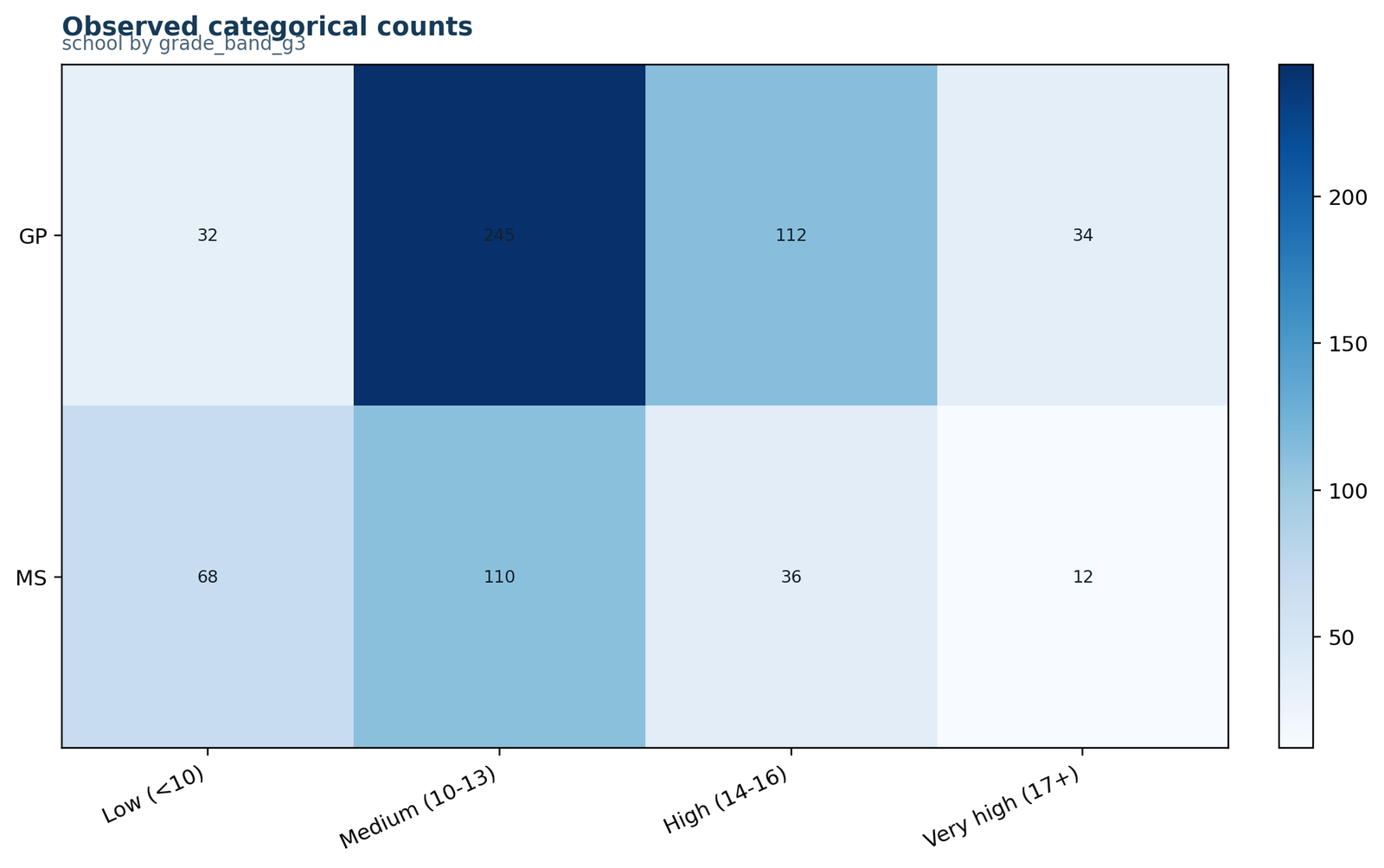
GP is largest in band 2, while MS has a much larger band 1 count than GP.
GP = 32, 245, 112, 34; MS = 68, 110, 36, 12.
The raw table suggests different grade-band profiles across schools.
Observed counts are the empirical foundation for every expected count and test statistic.
Chart 2: Likelihood Ratio Chi Square expected countsPython
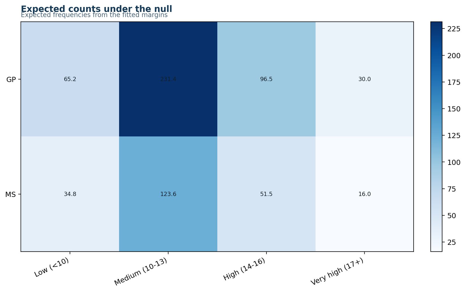
The expected table smooths the grade-band distribution according to the row and column margins.
Expected GP band 1 = 65.18 and expected MS band 1 = 34.82.
The observed band 1 counts of 32 and 68 are almost reversed relative to expectation.
The independence model is evaluated by comparing every observed cell with these expected counts.
Chart 3: Likelihood Ratio Chi Square Pearson residualsPython
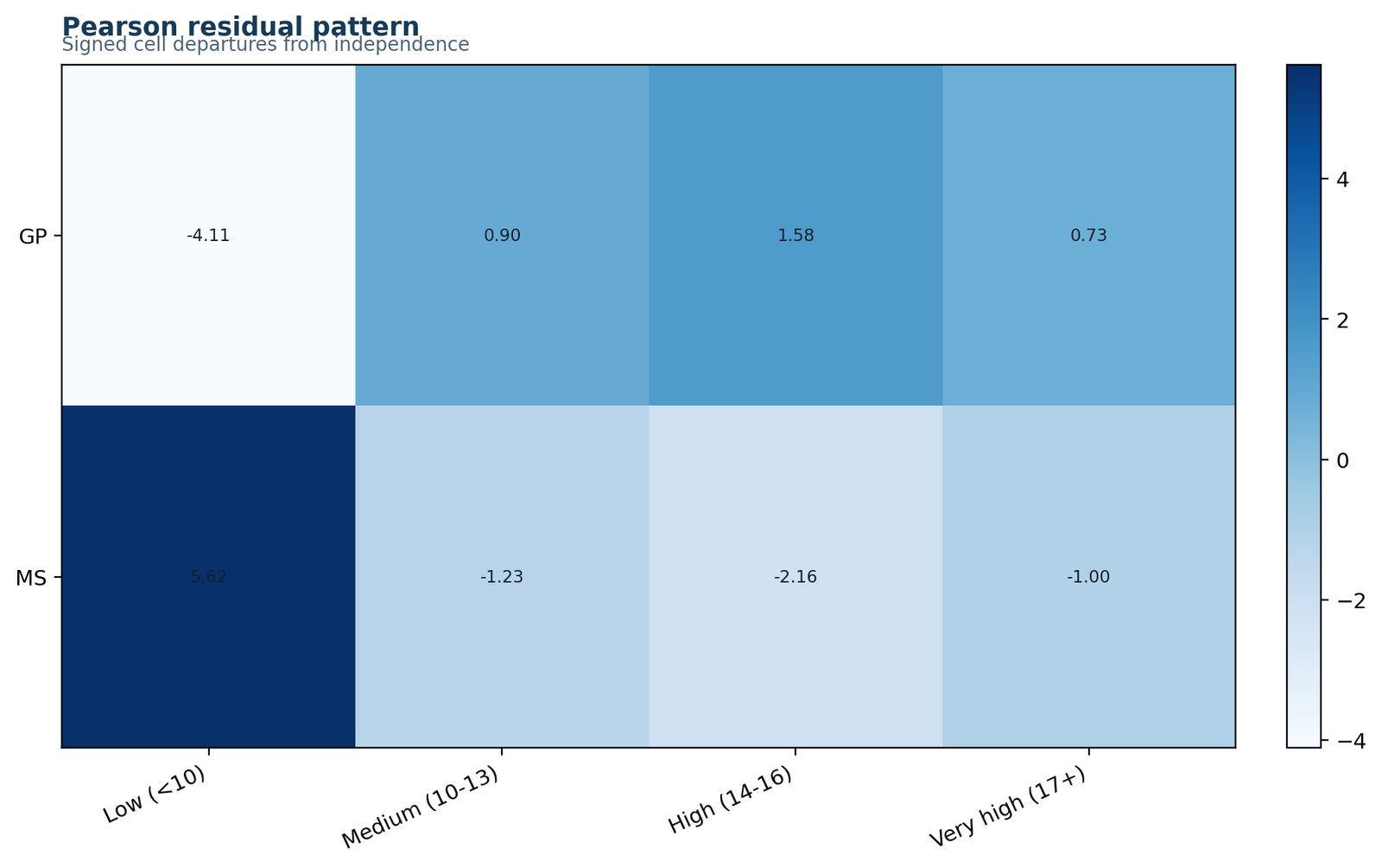
MS band 1 has the largest positive residual, while GP band 1 has the largest negative residual.
Residuals are −4.11 and +5.62 for band 1, and MS band 3 is −2.16.
Positive residuals indicate overrepresentation; negative residuals indicate underrepresentation.
Residuals identify which cells drive a significant global test.
Chart 4: Likelihood Ratio Chi Square cell contributionsPython
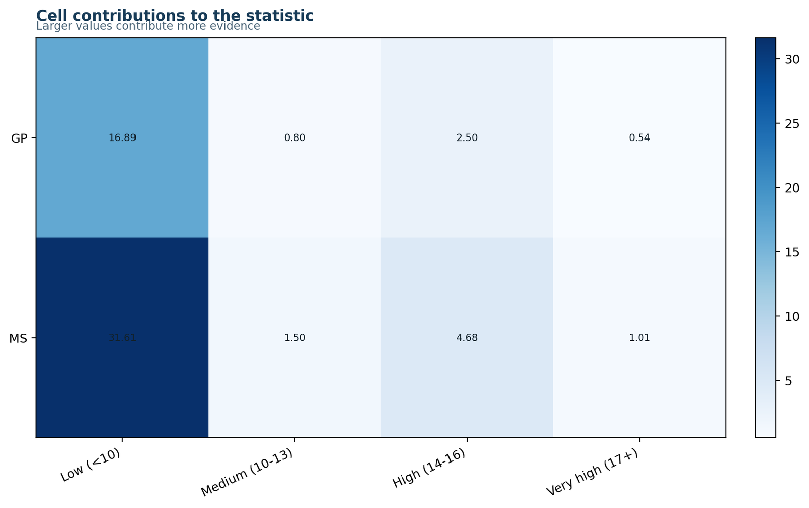
The grade-band 1 cells dominate the likelihood-ratio decomposition.
GP band 1 contributes −45.53 and MS band 1 contributes +91.02 before all signed terms are summed.
The signs show direction, while the total of all terms gives the nonnegative deviance.
The chart connects the global statistic to specific school-by-band combinations.
Chart 5: Likelihood Ratio Chi Square row percentagesPython
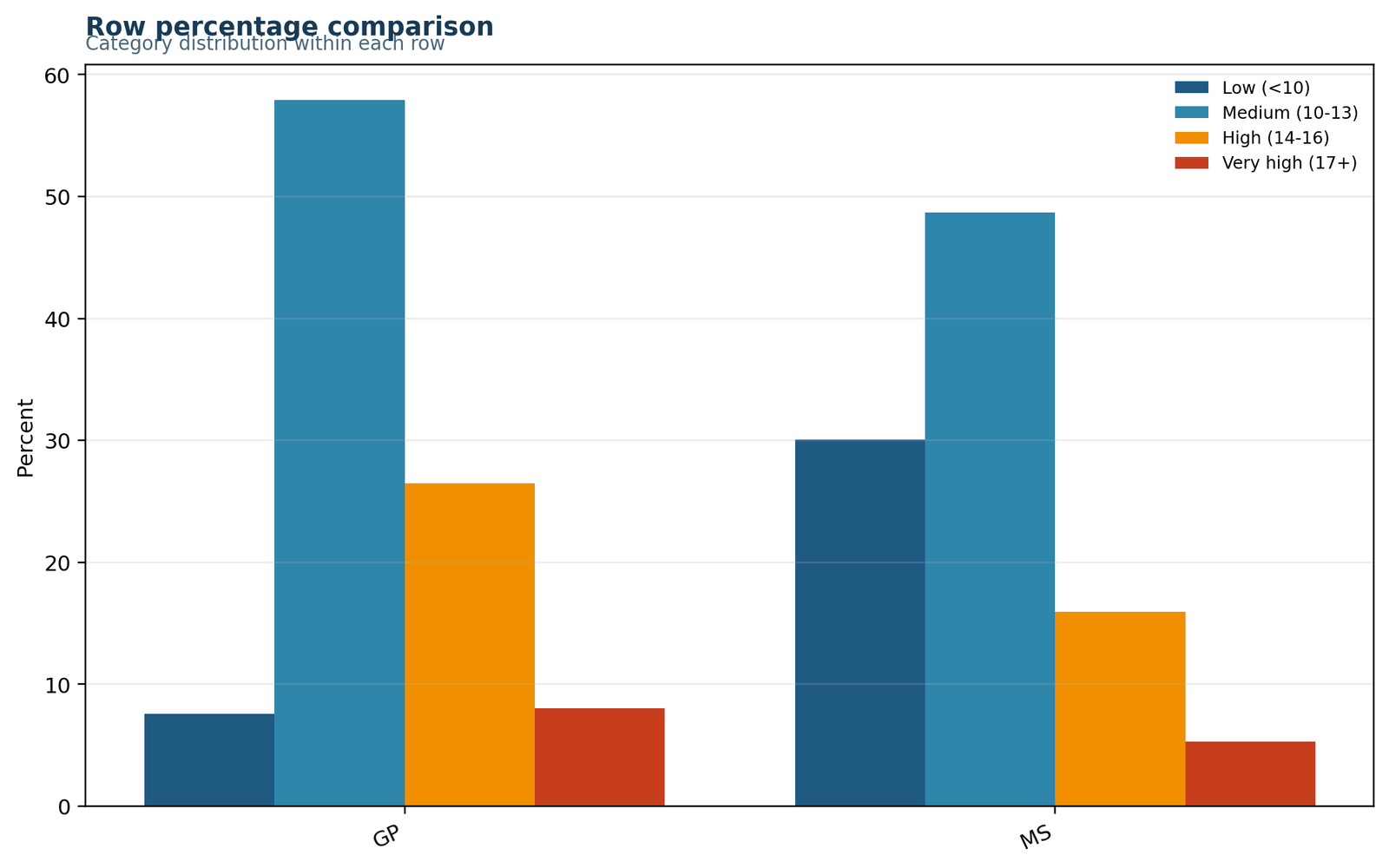
Band 1 accounts for 30.09% of MS students but only 7.57% of GP students.
GP: 7.57%, 57.92%, 26.48%, 8.04%; MS: 30.09%, 48.67%, 15.93%, 5.31%.
The school profiles differ most strongly in the lowest grade band.
Percentages communicate the substantive association more clearly than raw counts alone.
Chart 6: Likelihood Ratio Chi Square model diagnosticsPython
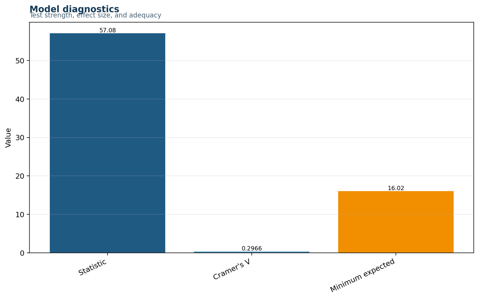
Every expected count is well above the common threshold of 5.
Minimum expected count = 16.0185; cells below 5 = 0.
The asymptotic chi-square reference is well supported for this table.
Diagnostics determine whether the reported p-value is based on a reasonable approximation.
Chart 7: Likelihood Ratio Chi Square versus Pearson chi-squarePython
The two statistics are close and both are far beyond the rejection threshold.
G² = 57.0752 and Pearson X² = 59.5340.
Both discrepancy measures reject independence decisively.
Agreement between methods supports a robust inferential conclusion.
Six R Likelihood Ratio Chi Square Charts in Paired Rows
The R workflow presents the observed and expected tables, residuals, likelihood contributions, row profiles and final result summary in three balanced pairs.
R pair 1: Likelihood Ratio Chi Square observed and expected counts
Observed band 1 counts differ sharply
GP has only 32 band 1 students compared with 65.18 expected, while MS has 68 compared with 34.82 expected.
The margins define the null model
The expected chart shows what the table would look like if school and grade band were independent but the observed row and column totals stayed fixed.
R pair 2: Likelihood Ratio Chi Square residuals and contributions
Residuals isolate the unusual cells
MS band 1 is strongly overrepresented, GP band 1 is strongly underrepresented and MS band 3 is moderately underrepresented.
Likelihood terms explain the deviance
The signed likelihood components show how each cell changes the log-likelihood difference between the independence and saturated models.
R pair 3: Likelihood Ratio Chi Square row profiles and result summary
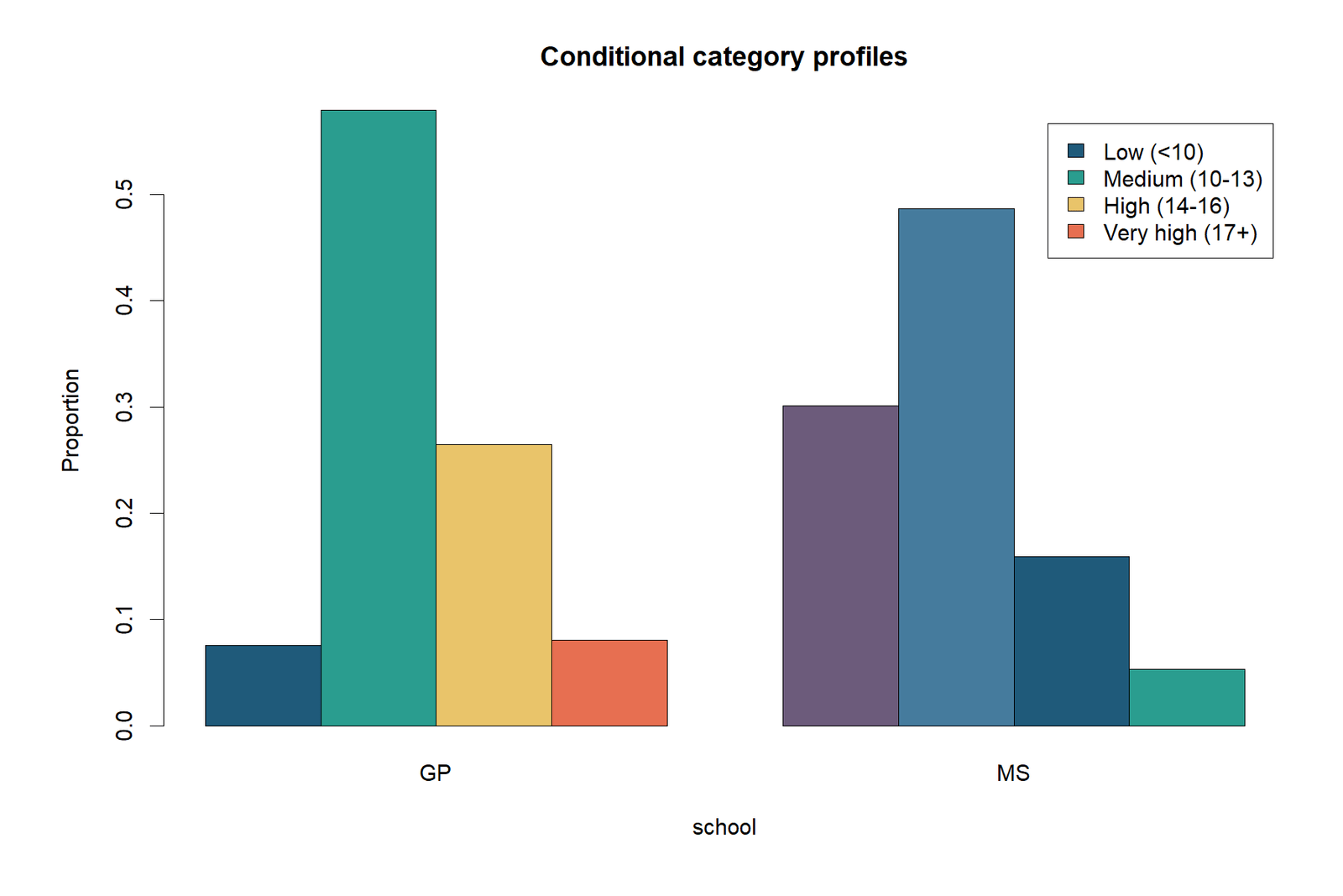
The school profiles are visibly different
MS has a much larger share in band 1 and smaller shares in bands 2, 3 and 4. GP is concentrated more heavily in bands 2 and 3.
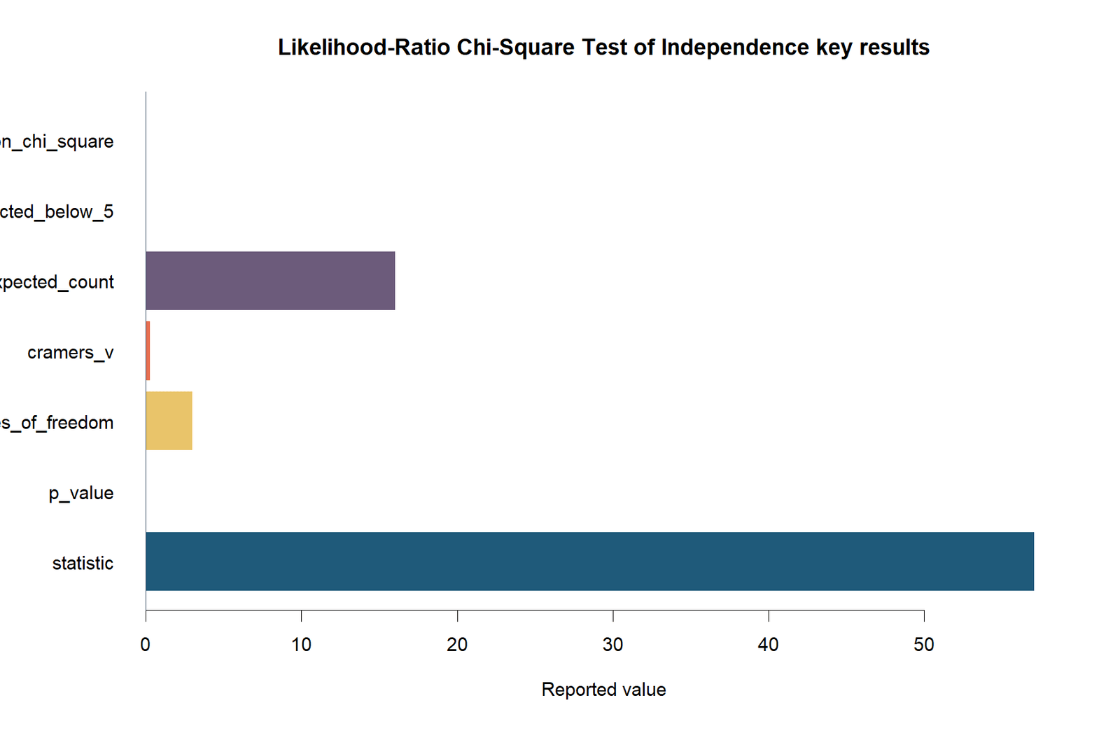
The global inference and effect size agree
The summary chart reports an extremely small p-value and a moderate Cramér’s V, combining statistical evidence with magnitude.
Likelihood Ratio Chi Square in Python, R, SPSS, SAS and Excel
Likelihood Ratio Chi Square in Python
Python can calculate expected counts, Pearson residuals, likelihood components, G², Pearson X², p-values and Cramér’s V from the same 2 × 4 table. See categorical data analysis in Python.
- Build the observed count matrix.
- Calculate margins and expected counts.
- Compute 2O ln(O/E) cell terms.
- Use the chi-square survival function with df = 3.
- Create diagnostics and comparison charts.
Likelihood Ratio Chi Square in R
R can obtain both Pearson and likelihood-ratio results through contingency-table and log-linear modeling workflows. See categorical data analysis in R.
- Create a matrix with schools in rows and bands in columns.
- Fit an independence model or compute G² manually.
- Extract expected counts and residuals.
- Calculate Cramér’s V.
- Generate paired diagnostic charts.
Likelihood Ratio Chi Square in SPSS
SPSS CROSSTABS reports Pearson Chi-Square and Likelihood Ratio in the Chi-Square Tests table. See categorical data analysis in SPSS.
- Place school in rows and grade band in columns.
- Request observed counts, expected counts and row percentages.
- Request chi-square statistics.
- Inspect the Likelihood Ratio row.
- Report effect size and residual diagnostics separately.
Likelihood Ratio Chi Square in SAS
SAS PROC FREQ reports likelihood-ratio chi-square for contingency tables and can produce expected counts and association measures.
- Specify the two-way table.
- Request CHISQ and association measures.
- Inspect the likelihood-ratio statistic and df.
- Confirm category order.
- Export output with ODS.
Likelihood Ratio Chi Square in Excel
The worked Excel file reproduces the observed table, expected counts, likelihood-ratio components, Pearson residuals, diagnostics and reporting summary.
- Calculate row, column and grand totals.
- Use row total × column total / N for expected counts.
- Use 2*O*LN(O/E) for each nonzero cell.
- Sum all terms for G².
- Use CHISQ.DIST.RT for the p-value.
Likelihood Ratio Chi Square in Stata and log-linear models
Stata and other statistical systems can obtain the same statistic through tabulation or log-linear model deviance. The modeling route is especially useful when the table is part of a larger categorical model.
- Declare categorical variables correctly.
- Fit the independence model.
- Compare deviance with the saturated model.
- Match degrees of freedom to the parameter difference.
- Report software and version.
Expandable Code for Likelihood Ratio Chi Square
Python pseudo-code
observed = [[32, 245, 112, 34],
            [68, 110, 36, 12]]
row_totals = observed.sum(axis=1)
col_totals = observed.sum(axis=0)
N = observed.sum()
expected = outer(row_totals, col_totals) / N
G2 = 2 * sum(observed * log(observed / expected))
df = (observed.shape[0]-1) * (observed.shape[1]-1)
p = chi2.sf(G2, df)
R pseudo-code
tab <- matrix(c(32,245,112,34,68,110,36,12), nrow=2, byrow=TRUE)
expected <- outer(rowSums(tab), colSums(tab)) / sum(tab)
G2 <- 2 * sum(tab * log(tab / expected))
df <- (nrow(tab)-1) * (ncol(tab)-1)
p <- pchisq(G2, df=df, lower.tail=FALSE)
SPSS syntax idea
CROSSTABS
 /TABLES=school BY grade_band
 /STATISTICS=CHISQ PHI
 /CELLS=COUNT EXPECTED ROW RESID.
Excel formulas
=RowTotal*ColumnTotal/GrandTotal
=IF(Observed=0,0,2*Observed*LN(Observed/Expected))
=SUM(AllLikelihoodComponents)
=CHISQ.DIST.RT(G2,DegreesOfFreedom)
Assumptions, Diagnostics and Advanced Interpretation
Core assumptions
- Each observation belongs to one and only one cell.
- Subjects are independent.
- Categories are mutually exclusive.
- Expected counts are adequate for asymptotic inference.
- The variables are categorical and correctly coded.
Model diagnostics
- Minimum expected count = 16.0185.
- Cells with expected count below 5 = 0.
- Sample size = 649.
- Pearson and likelihood-ratio results agree.
- Residuals identify the main departures.
Likelihood Ratio Chi Square with zero cells and logarithms
A zero observed count does not make the entire statistic undefined. Its contribution is treated as zero by the limiting definition. A zero expected count is different and indicates a structural problem with the null model or category definition.
Likelihood Ratio Chi Square with large samples and tiny p-values
With large samples, even modest discrepancies can become statistically significant. That is why Cramér’s V and row percentages are essential. Here, the effect is not trivial: V is close to .30, and the band 1 percentages differ by more than 22 percentage points.
Likelihood Ratio Chi Square with ordered categories
The grade bands are ordered, but the basic Likelihood Ratio Chi Square treats them as nominal categories. It does not use the ordering information. If the research question concerns trend or ordinal association, an ordinal model or a score-based test may be more efficient.
Likelihood Ratio Chi Square and log-linear models
The independence model is a log-linear model with row and column main effects but no interaction. The saturated model includes the school-by-grade-band interaction and fits the observed table exactly. G² measures the deviance lost by omitting that interaction. This model perspective explains why the statistic is called a likelihood-ratio test.
APA Reporting for Likelihood Ratio Chi Square
Significant worked-example report
Significant
A Likelihood Ratio Chi Square test of independence was conducted to examine the association between school and G3 grade band.
The association was statistically significant, G²(3, N = 649) = 57.08, p < .001, Cramér’s V = .297.
MS students were overrepresented in grade band 1, whereas GP students were underrepresented in that band and more concentrated in bands 2 and 3.
Include the row percentages or residual pattern after the inferential sentence.
Reusable general template
Template
A Likelihood Ratio Chi Square test of independence examined the association between row variable and column variable.
The association was significant/not significant, G²(df, N = N) = statistic, p = p-value, Cramér’s V = effect size.
The strongest departures occurred in cells or categories.
Short table-note version
Concise
School and G3 grade band were associated, G²(3, N = 649) = 57.08, p < .001, V = .297.
Common Likelihood Ratio Chi Square Mistakes and How to Correct Them
Common mistakes
- Calling the statistic an odds ratio or diagnostic likelihood ratio.
- Reporting it without expected counts or residuals.
- Choosing between Pearson and G² after seeing the p-values.
- Ignoring small expected counts.
- Interpreting significance as causation.
- Failing to state which variables define rows and columns.
- Using nominal analysis when an ordinal model is required.
How to correct them
- Use the full name Likelihood Ratio Chi Square or G-squared.
- Include observed, expected and percentage tables.
- Prespecify the primary method.
- Check minimum expected counts and sparse cells.
- Describe association, not causal effect.
- Document coding and category order.
- Use an ordinal method when trend is the target.
Likelihood Ratio Chi Square Reports and Worked Excel Download
R PDF reportR analysis and paired visual interpretation for the same 2 × 4 table.
SPSS PDF outputSPSS Likelihood Ratio and Pearson chi-square output.
Worked Excel analysisTransparent formulas, expected counts, residuals, diagnostics and reporting sheet.
Frequently Asked Questions About Likelihood Ratio Chi Square
What is Likelihood Ratio Chi Square?
It is a contingency-table test that compares the likelihood of an independence model with the likelihood of a saturated model. The test statistic is commonly written as G².
How do I interpret a significant Likelihood Ratio Chi Square?
A significant result means the two categorical variables are associated and the independence model does not fit. Residuals and percentages are then used to explain the pattern.
What is the formula?
G² = 2 Σ O ln(O/E), summed across all cells of the contingency table.
Why does it have a chi-square distribution?
Under regularity conditions, twice the log-likelihood difference between nested models follows an asymptotic chi-square distribution, with degrees of freedom equal to the difference in model parameters.
When should I use Pearson chi-square instead?
Both are valid for well-behaved tables. Pearson is traditional for residual-based analysis, while the likelihood-ratio statistic is natural for deviance and log-linear modeling. Choose the primary method before viewing results.
What does SPSS Likelihood Ratio mean?
In the SPSS Chi-Square Tests table, the Likelihood Ratio row reports the G-squared statistic, its degrees of freedom and asymptotic significance.
Can Likelihood Ratio Chi Square be used with small expected counts?
The statistic can be computed, but the asymptotic p-value may be unreliable. An exact or Monte Carlo procedure may be preferable for sparse tables.
How should the worked result be reported?
School and G3 grade band were associated, G²(3, N = 649) = 57.08, p < .001, Cramér’s V = .297.
Likelihood Ratio Chi Square Conclusion
Likelihood Ratio Chi Square provides a likelihood-based test of categorical independence and connects ordinary contingency-table analysis with log-linear modeling and deviance. In the worked school-by-grade-band table, the independence model failed decisively, G²(3, N = 649) = 57.08, p < .001, Cramér’s V = .297.
The main practical finding is that MS students are substantially overrepresented in grade band 1, while GP students are underrepresented there and more heavily represented in higher bands. Pearson chi-square reaches the same conclusion, and the expected-count diagnostics are fully satisfactory. A complete report should therefore combine the Likelihood Ratio Chi Square statistic with expected counts, residuals, row percentages and effect size.
Continue with Chi Square Test of Independence, Chi Square Assumptions, Cramér’s V and AP Statistics Formula Sheet for related categorical-inference guidance.

