
Kappa Statistic: Formula, Interpretation, Calculator, Python, R, SPSS, SAS and Excel Guide
Kappa Statistic measures agreement between two raters, classifiers, occasions or diagnostic decisions after removing the agreement expected from their marginal distributions. This complete guide explains the Kappa Statistic formula, interpretation, calculator workflow, prevalence and bias effects, APA reporting, six Python charts, six R charts, SPSS, SAS and Excel workflows, code and downloadable reports through a worked binary agreement study of 649 students.
Observed agreement 89.68%
Kappa = 0.6655
PABAK = 0.7935
Kappa Statistic Model Overview
What is a kappa statistic? The kappa statistic is a chance-corrected measure of agreement for categorical classifications. Percent agreement counts how often two classifications are identical. The kappa statistic goes one step further by estimating how much agreement would be expected from the two marginal category distributions and then expressing the agreement beyond that chance benchmark as a proportion of the maximum possible improvement.
The worked example compares two binary pass/fail classifications derived from the same students: G2 ≥ 10 and G3 ≥ 10. Every row contributes one G2 classification and one G3 classification. Because both decisions refer to the same student, the classifications are paired. The analysis therefore concerns agreement, not two independent proportions and not association between unrelated groups.
What question does the kappa statistic answer?
The inferential question is whether the agreement between the G2 and G3 pass/fail classifications exceeds the agreement expected from their margins. The descriptive question is how strong the agreement is after chance correction. These questions are related but not identical: the p-value tests whether kappa is greater than zero, while the estimated kappa statistic quantifies the magnitude of agreement.
How the chance correction works
If both classifications label most students as passing, high raw agreement can occur even when the two decisions are not especially concordant beyond their margins. The kappa statistic compares observed agreement Po with expected agreement Pe. In this dataset, observed agreement is 0.8968, but the unequal pass/fail margins already imply expected agreement of 0.6913. The kappa statistic therefore reports the proportion of possible agreement beyond chance that was actually achieved.
Worked example at a glance
The 2 × 2 agreement table contains 89 students classified as failing on both occasions, 493 classified as passing on both occasions, 56 who moved from G2 fail to G3 pass and 11 who moved from G2 pass to G3 fail. There are 582 exact agreements and 67 disagreements. The resulting kappa statistic is 0.665528, with a 95% confidence interval from 0.592652 to 0.738405 and a two-sided p-value of 8.341893 × 10−68.
Quick Answer: Kappa Statistic Result
The primary analysis is an unweighted binary kappa statistic for two paired classifications. The same 649 students are classified by G2 pass/fail and G3 pass/fail using the threshold 10.
Statistical summary
- Procedure: binary unweighted kappa statistic
- Observed agreement: 0.896764
- Expected agreement: 0.691347
- Kappa: 0.665528
- Standard error: 0.037183
- 95% CI: [0.592652, 0.738405]
- z: 17.3994
- Decision: reject H0: κ = 0
Agreement diagnostics
- PABAK: 0.793529
- Prevalence index: 0.622496
- Bias index: 0.069337
- Positive agreement: 0.936372
- Negative agreement: 0.726531
- Maximum possible κ with these margins: 0.775355
- Achieved fraction of maximum κ: 85.84%
Table of Contents
- Research question, hypotheses and data design
- When to use the Kappa Statistic
- Kappa Statistic formula and calculation
- Variables and data dictionary
- Worked 2 × 2 agreement table and complete results
- Kappa versus percent agreement, PABAK and alternatives
- Kappa Statistic calculator steps
- Twelve Python and R chart interpretations
- Python, R, SPSS, SAS and Excel workflows
- Expandable Kappa Statistic code
- Assumptions, prevalence, bias and advanced interpretation
- APA reporting for the Kappa Statistic
- Common Kappa Statistic mistakes and corrections
- Reports and worked Excel download
- Related Salar Cafe guides
- Frequently asked questions
- Kappa Statistic conclusion
Research Question, Hypotheses and Data Design
Research question
How strongly do the G2 and G3 pass/fail classifications agree after correcting for agreement expected from their marginal distributions?
Null and alternative hypotheses
| Hypothesis | Statistical statement | Meaning |
|---|---|---|
| Null hypothesis | H0: κ = 0 | The classifications agree only at the level expected from their margins. |
| Two-sided alternative | H1: κ ≠ 0 | Agreement differs from chance expectation. |
| Directional alternative | H1: κ > 0 | Agreement is greater than chance; use only when prespecified. |
Why this is an agreement problem
A chi-square test of independence asks whether two categorical variables are associated. The kappa statistic asks a stricter question: do the paired classifications assign the same category to the same cases more often than expected? A strong association can exist without strong exact agreement, so association and agreement must not be treated as synonyms.
Why the data must remain paired
The 649 G2 classifications cannot be compared with the 649 G3 classifications as if they were independent groups. Each G2 decision is linked to the G3 decision for the same student. The off-diagonal cells describe the direction of within-student disagreement and are essential for prevalence, bias and concordance diagnostics.
When to Use the Kappa Statistic
Use the kappa statistic when
- The same cases are classified by two raters, tests, algorithms or occasions.
- The outcome categories are nominal or binary.
- You need agreement rather than simple association.
- Every case has one classification from each source.
- The category labels have the same meaning for both classifications.
- You want chance-corrected interrater or test–retest reliability.
- You are evaluating medical diagnoses, coding decisions, machine-learning labels, map classifications or educational categories.
Choose another method when
- There are more than two raters and one common multi-rater coefficient is needed.
- Categories are ordered and the size of disagreement should receive weights.
- The outcome is continuous; then an intraclass correlation coefficient may be more appropriate.
- The groups are independent rather than paired.
- You need sensitivity, specificity or predictive performance against a true gold standard.
- Missing classifications are extensive or not missing at random.
- The category set differs between the two raters.
Simple method-selection logic
Use kappa when identical classifications are the target.
Two paired classifications support Cohen-type kappa; more raters require a multi-rater extension.
Use unweighted kappa for nominal categories and weighted kappa when ordinal distance matters.
Binary kappa statistic versus diagnostic accuracy
When neither classification is a gold standard, the kappa statistic is a symmetric agreement measure. If G3 were declared the truth and G2 were treated as a prediction, the same table could also produce sensitivity, specificity, predictive values and accuracy. Those metrics answer a different question because they assign different roles to the two classifications. The kappa statistic does not require one source to be correct.
Kappa statistic in machine learning
In machine learning, the kappa statistic is often calculated from a confusion matrix to compare predicted labels with reference labels while accounting for class prevalence. It should be accompanied by class-specific performance because severe imbalance can produce a high accuracy but a lower kappa value. For modelling alternatives, see logistic regression and multinomial logistic regression.
Kappa Statistic Formula and Calculation
The basic kappa statistic formula is:
Po is observed agreement and Pe is expected agreement calculated from the row and column margins.
Step 1: Build the agreement matrix
| G2 pass classification | G3 fail (0) | G3 pass (1) | Row total |
|---|---|---|---|
| G2 fail (0) | 89 | 56 | 145 |
| G2 pass (1) | 11 | 493 | 504 |
| Column total | 100 | 549 | 649 |
Step 2: Calculate observed agreement
The observed agreement is 89.6764%. The disagreement rate is 67/649 = 10.3236%.
Step 3: Calculate expected agreement from the margins
In count units, the margins imply approximately 22.34 chance agreements in the fail category and 426.34 chance agreements in the pass category, for 448.68 expected diagonal agreements overall.
Step 4: Calculate the kappa statistic
The numerator, 0.2054174, is the observed agreement above chance. The denominator, 0.3086531, is the maximum improvement available above the expected agreement benchmark.
Step 5: Calculate uncertainty and significance
| Quantity | Value | Meaning |
|---|---|---|
| Standard error of κ | 0.0371826 | Estimated sampling variability of the kappa statistic. |
| 95% lower confidence limit | 0.5926517 | Lower plausible value under the asymptotic interval. |
| 95% upper confidence limit | 0.7384048 | Upper plausible value under the asymptotic interval. |
| z statistic for H0: κ = 0 | 17.3994 | Large standardized departure from zero agreement beyond chance. |
| Two-sided p-value | 8.341893 × 10−68 | Reject the zero-kappa null. |
Step 6: Calculate PABAK
Prevalence-adjusted bias-adjusted kappa replaces the observed margins with balanced margins. It is not a universal replacement for the kappa statistic. It is a sensitivity diagnostic showing how much the conventional kappa estimate is affected by prevalence and marginal imbalance.
Step 7: Calculate prevalence and bias indices
The large prevalence index reflects the dominance of the pass/pass cell over the fail/fail cell. The smaller bias index reflects the difference between the two directions of disagreement.
Step 8: Calculate positive and negative agreement
Agreement is considerably stronger for passing than for failing. This asymmetry is hidden when only the overall kappa statistic is reported.
Variables and Data Dictionary
| Variable | Role | Original scale | Binary coding | Meaning |
|---|---|---|---|---|
| G2 | First classification source | Second-period grade | 0 when G2 < 10; 1 when G2 ≥ 10 | First pass/fail decision for each student. |
| G3 | Second classification source | Final grade | 0 when G3 < 10; 1 when G3 ≥ 10 | Second pass/fail decision for the same student. |
| Student row | Matched unit | One student | One paired classification | Preserves the pairing needed for agreement analysis. |
Marginal classification profiles
| Classification source | Fail count | Pass count | Fail proportion | Pass proportion |
|---|---|---|---|---|
| G2 | 145 | 504 | 0.223421 | 0.776579 |
| G3 | 100 | 549 | 0.154083 | 0.845917 |
The G3 classification labels 45 more students as passing than the G2 classification. That difference appears in the off-diagonal counts: 56 students move from G2 fail to G3 pass, whereas 11 move from G2 pass to G3 fail. The bias index of 0.0693 summarizes this directional imbalance.
For foundational table-reading skills, see cross-tabulation, frequency distribution and descriptive statistics.
Worked 2 × 2 Agreement Table and Complete Results
13.71% of all cases
75.96% of all cases
89.68%
10.32%
Chance-corrected agreement
Balanced-margin sensitivity diagnostic
Primary kappa statistic result
| Metric | Estimate | 95% confidence interval | Interpretation |
|---|---|---|---|
| Observed agreement | 0.896764 | — | 89.68% of paired classifications match exactly. |
| Expected agreement | 0.691347 | — | Agreement expected from the marginal pass/fail rates. |
| Kappa statistic | 0.665528 | [0.592652, 0.738405] | Strong agreement beyond chance. |
| Maximum attainable kappa | 0.775355 | — | Upper limit imposed by unequal margins. |
| κ / κmax | 0.858353 | — | About 85.84% of margin-constrained maximum agreement achieved. |
Statistical interpretation
The two-sided p-value is far below .001, so the null hypothesis of zero agreement beyond chance is rejected. Statistical significance is unsurprising with 649 paired observations and κ = 0.666. The confidence interval provides more information than the p-value because it shows that plausible population values range from approximately 0.593 to 0.738.
Substantive interpretation
The classifications agree particularly well on passing students. Positive agreement is 93.64%, whereas negative agreement is 72.65%. The lower negative agreement indicates that the fail classification is less stable across G2 and G3. This may reflect improvement between grading periods, threshold sensitivity, measurement variability or genuine change in performance.
Prevalence and bias interpretation
The conventional kappa statistic is lower than PABAK because passing is common. The prevalence index of 0.6225 is large, while the bias index of 0.0693 is much smaller. This pattern is often called a prevalence effect: high agreement occurs mainly in one dominant category, increasing expected chance agreement and reducing κ relative to raw agreement.
Kappa Statistic Versus Percent Agreement, PABAK and Alternative Methods
Simple proportion of exact matches; does not correct for expected agreement.
Corrects exact agreement using the marginal category distributions.
Allows smaller penalties for near disagreements when categories are ordered.
Reliability measure for quantitative ratings rather than nominal categories.
Kappa statistic versus percent agreement
| Measure | Value | What it captures | Main limitation |
|---|---|---|---|
| Percent agreement | 89.68% | Observed exact matches. | Ignores chance expectation from margins. |
| Kappa statistic | 0.6655 | Agreement beyond marginal chance. | Sensitive to prevalence and marginal imbalance. |
| PABAK | 0.7935 | Agreement under balanced prevalence and bias assumptions. | Changes the margin model and should be labelled clearly. |
| Positive agreement | 93.64% | Agreement specifically on the pass classification. | Does not summarize fail agreement. |
| Negative agreement | 72.65% | Agreement specifically on the fail classification. | Does not summarize pass agreement. |
Unweighted versus weighted kappa statistic
The current categories are binary, so every disagreement receives the same penalty. With three or more ordered categories, weighted kappa can distinguish adjacent disagreement from extreme disagreement. Weight choice must be declared because linear and quadratic weighting can produce different kappa values.
Two-rater versus multi-rater agreement
The current kappa statistic compares two classification sources. Fleiss-type kappa extends agreement analysis to multiple raters when each item receives a fixed number of nominal classifications. It is not calculated by averaging every pairwise Cohen kappa without justification.
Kappa statistic versus intraclass correlation
For continuous measurements, use an intraclass correlation coefficient guide. ICC evaluates agreement or consistency in numerical ratings and requires choices about model, raters and unit of inference. The kappa statistic is designed for categorical labels.
Kappa statistic versus chi-square, phi and Cramer's V
Chi-square tests, phi coefficient and Cramer's V evaluate association. The kappa statistic evaluates exact agreement. Two classifiers could have a strong association while systematically disagreeing by category, so association coefficients cannot replace kappa.
Kappa Statistic Calculator: Step-by-Step Workflow
A dependable kappa statistic calculator should accept the full agreement matrix, compute row and column margins, report observed and expected agreement, return κ and its uncertainty, and display prevalence and bias diagnostics rather than only one coefficient.
Calculator inputs
| Input | Value | Meaning |
|---|---|---|
| Both fail | 89 | G2 fail and G3 fail. |
| G2 fail, G3 pass | 56 | Upward disagreement. |
| G2 pass, G3 fail | 11 | Downward disagreement. |
| Both pass | 493 | G2 pass and G3 pass. |
| Confidence level | 95% | Interval for the population kappa statistic. |
| Weighting | None | Binary nominal kappa statistic. |
Calculator step 1: Verify the matrix orientation
The two diagonal cells must represent agreement. If one classifier's category order is reversed, diagonal counts become off-diagonal counts and the computed kappa statistic becomes meaningless.
Calculator step 2: Check observed agreement
The calculator should report 582 exact matches and observed agreement of 0.896764. A different value indicates incorrect cell placement or missing cases.
Calculator step 3: Check expected agreement
The expected agreement should be 0.691347. This value must be calculated from both marginal profiles, not assumed to be 0.50 simply because there are two categories.
Calculator step 4: Check kappa and uncertainty
The target result is κ = 0.665528, standard error 0.037183, 95% CI [0.592652, 0.738405], z = 17.3994 and two-sided p = 8.341893 × 10−68.
Calculator step 5: Review prevalence and bias
The calculator should also show PABAK = 0.793529, prevalence index = 0.622496 and bias index = 0.069337. These diagnostics explain why the agreement coefficient is lower than the raw agreement rate.
Twelve Python and R Kappa Statistic Chart Interpretations
Chart 1: Agreement matrixPython
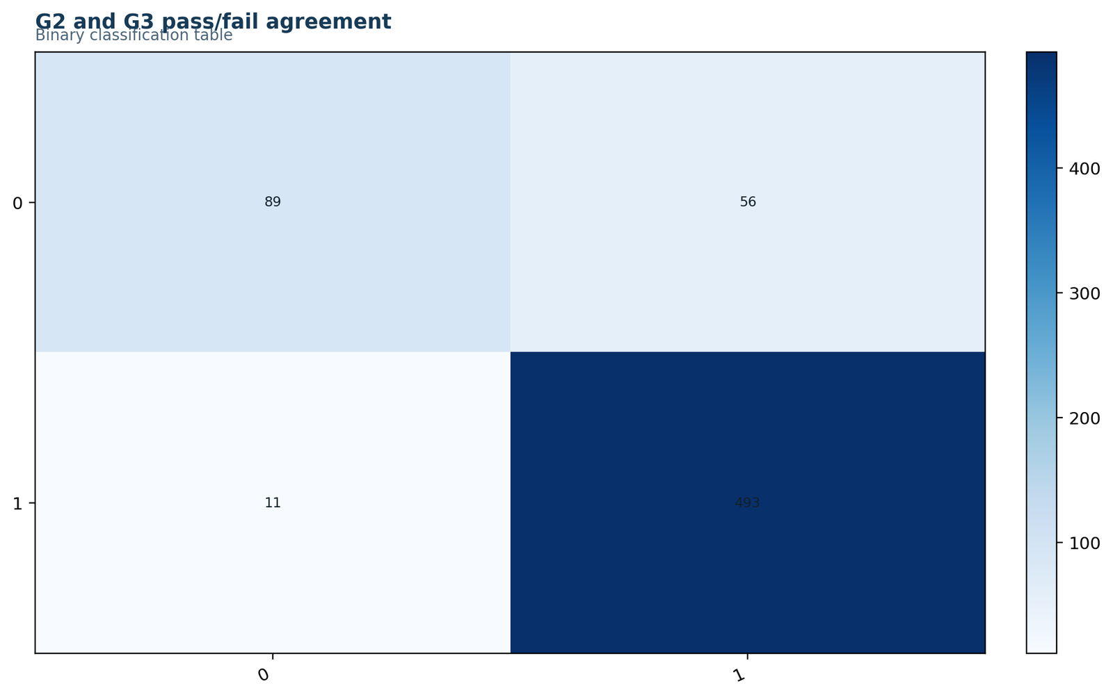
The dominant cell is pass/pass, followed by fail/fail. Upward disagreements are more common than downward disagreements.
Diagonal counts are 89 and 493; off-diagonal counts are 56 and 11.
Most students receive the same binary classification at G2 and G3, particularly in the pass category.
The agreement matrix is the source of every agreement coefficient, prevalence and bias calculation.
Chart 2: Cell countsPython
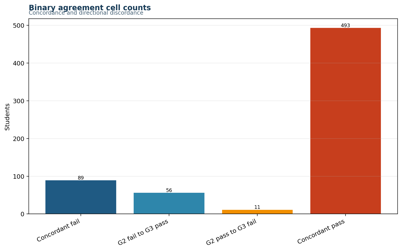
The pass/pass count is much larger than every other cell.
Both fail = 89, G2 fail/G3 pass = 56, G2 pass/G3 fail = 11, both pass = 493.
The asymmetric off-diagonal cells show that more students moved into passing than moved out of passing.
Direction of disagreement is clinically or educationally meaningful even when the overall agreement coefficient is strong.
Chart 3: Agreement measuresPython
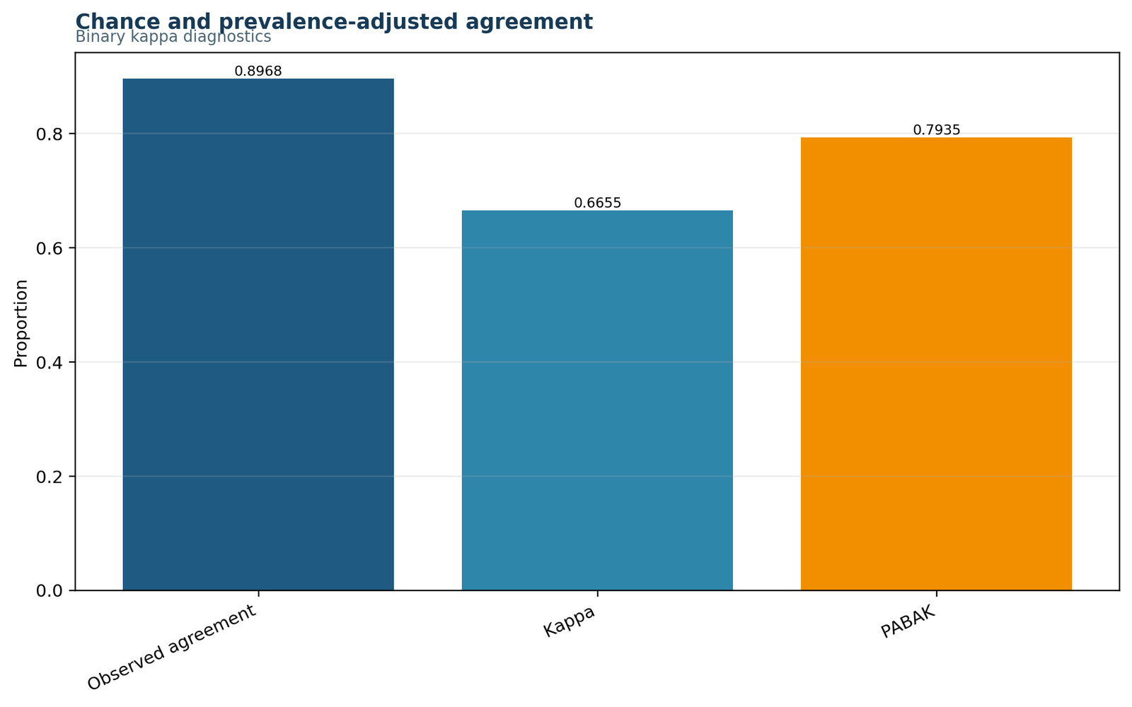
Observed agreement is highest, expected agreement is already substantial, and the conventional agreement coefficient lies below PABAK.
Po = 0.8968, Pe = 0.6913, κ = 0.6655 and PABAK = 0.7935.
The margins account for a large share of apparent agreement, but substantial agreement remains after correction.
Displaying all measures prevents raw agreement or PABAK from being mistaken for the conventional agreement coefficient.
Chart 4: Prevalence and bias diagnosticsPython
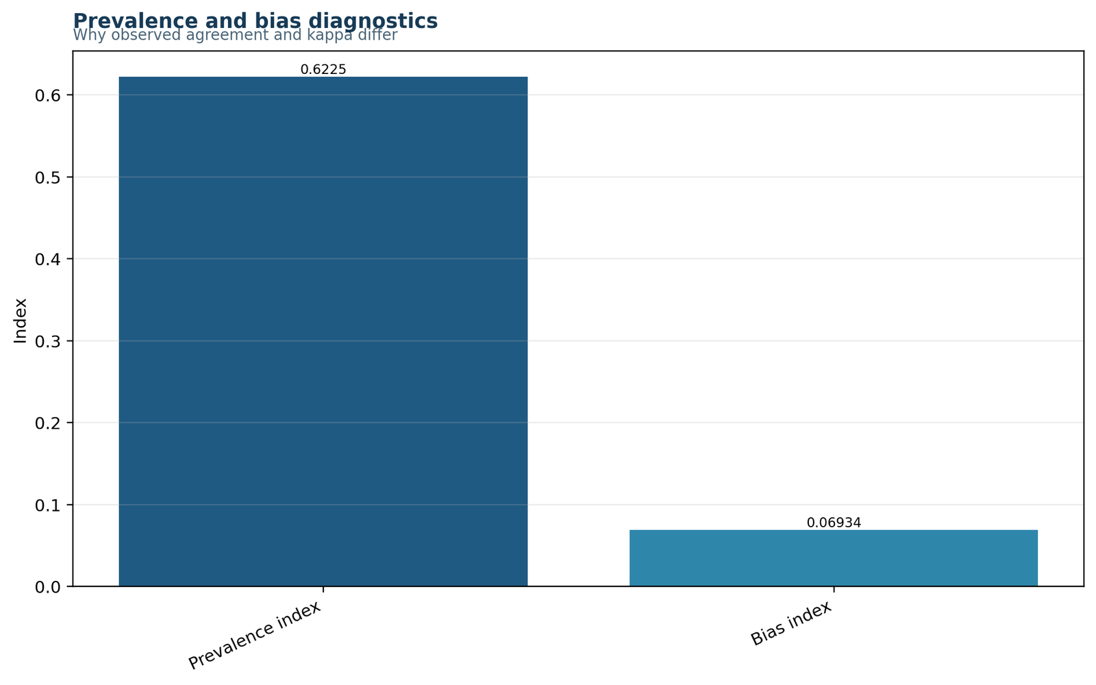
The prevalence index is much larger than the bias index.
Prevalence index = 0.6225 and bias index = 0.0693.
The dominant pass category has a stronger influence on kappa than disagreement-direction bias.
The prevalence diagnostic explains why high observed agreement can coexist with a lower chance-corrected coefficient.
Chart 5: Concordance balancePython
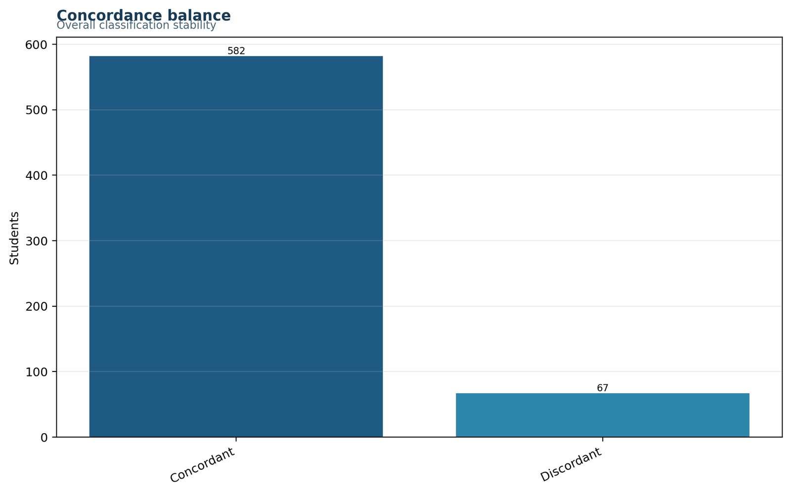
Positive agreement is markedly higher than negative agreement.
Positive agreement = 0.9364 and negative agreement = 0.7265.
The classifications are more reliable when identifying passing students than failing students.
One overall agreement coefficient cannot show this category-specific difference.
Chart 6: Result summaryPython
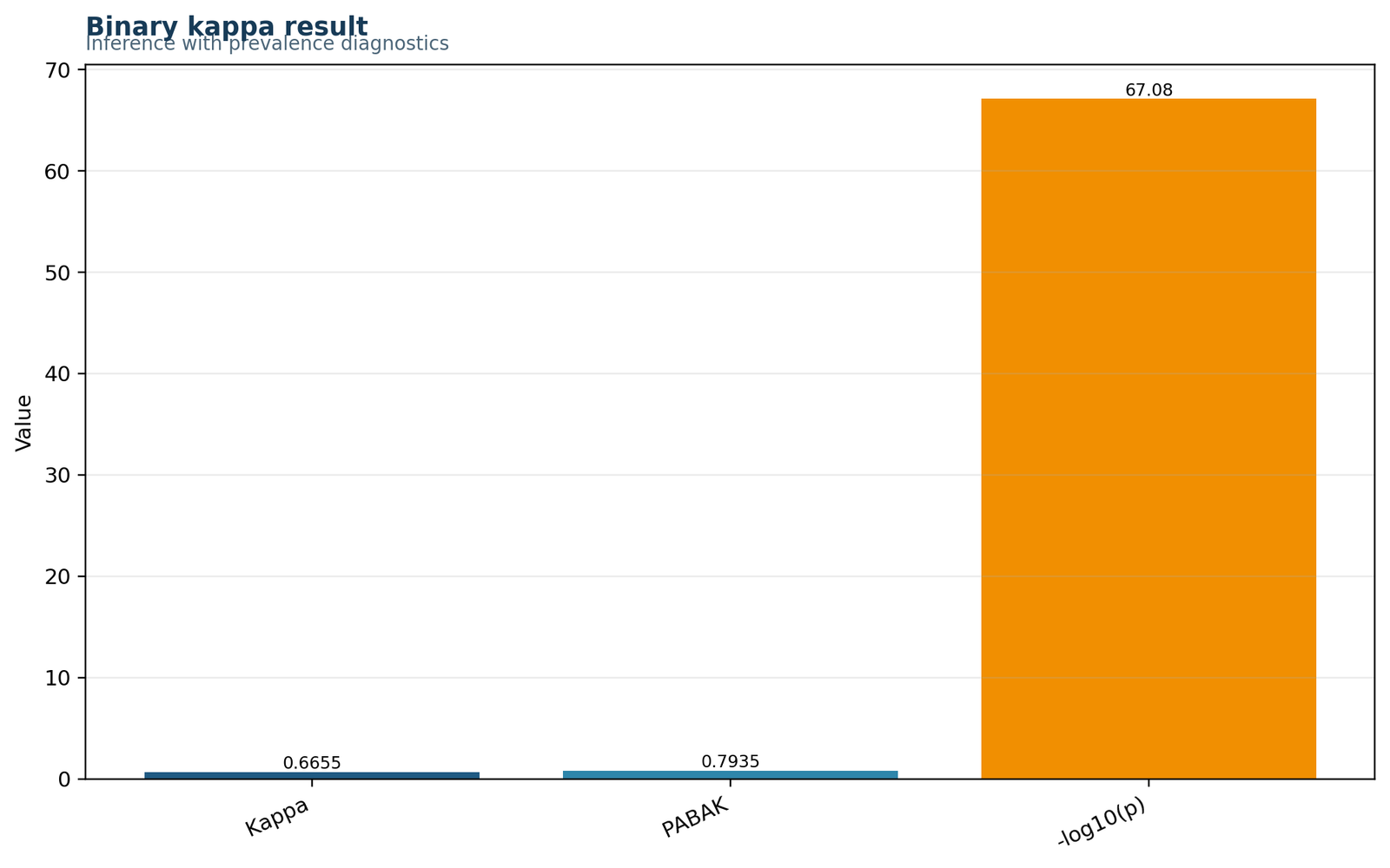
The summary panel consolidates the strong agreement result and the prevalence-sensitive diagnostics.
κ = 0.6655, 95% CI [0.5927, 0.7384], p < .001, PABAK = 0.7935.
Agreement beyond chance is statistically and substantively strong.
This chart provides a concise reporting view without hiding marginal imbalance.
R Kappa Statistic Chart Pairs
The R charts present the same binary agreement analysis in three paired rows. Each pair combines one structural view of the agreement table with one inferential or diagnostic view.
R pair 1: Agreement matrix and expected agreement
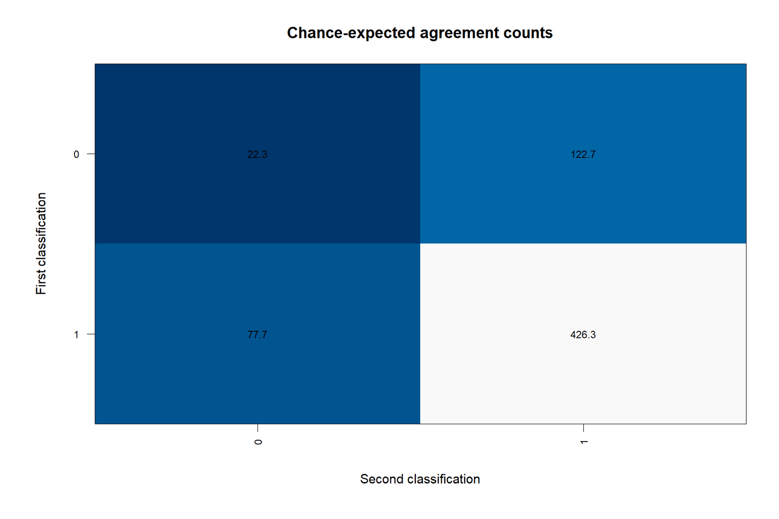
Agreement is concentrated on passing
The matrix contains 493 pass/pass agreements and 89 fail/fail agreements. The 56 versus 11 off-diagonal split shows directional change between G2 and G3.
The margins imply high expected agreement
Because both classifications label most students as passing, chance agreement is already 0.6913. Most expected agreement comes from the pass/pass component.
R pair 2: Diagonal counts and marginal profiles
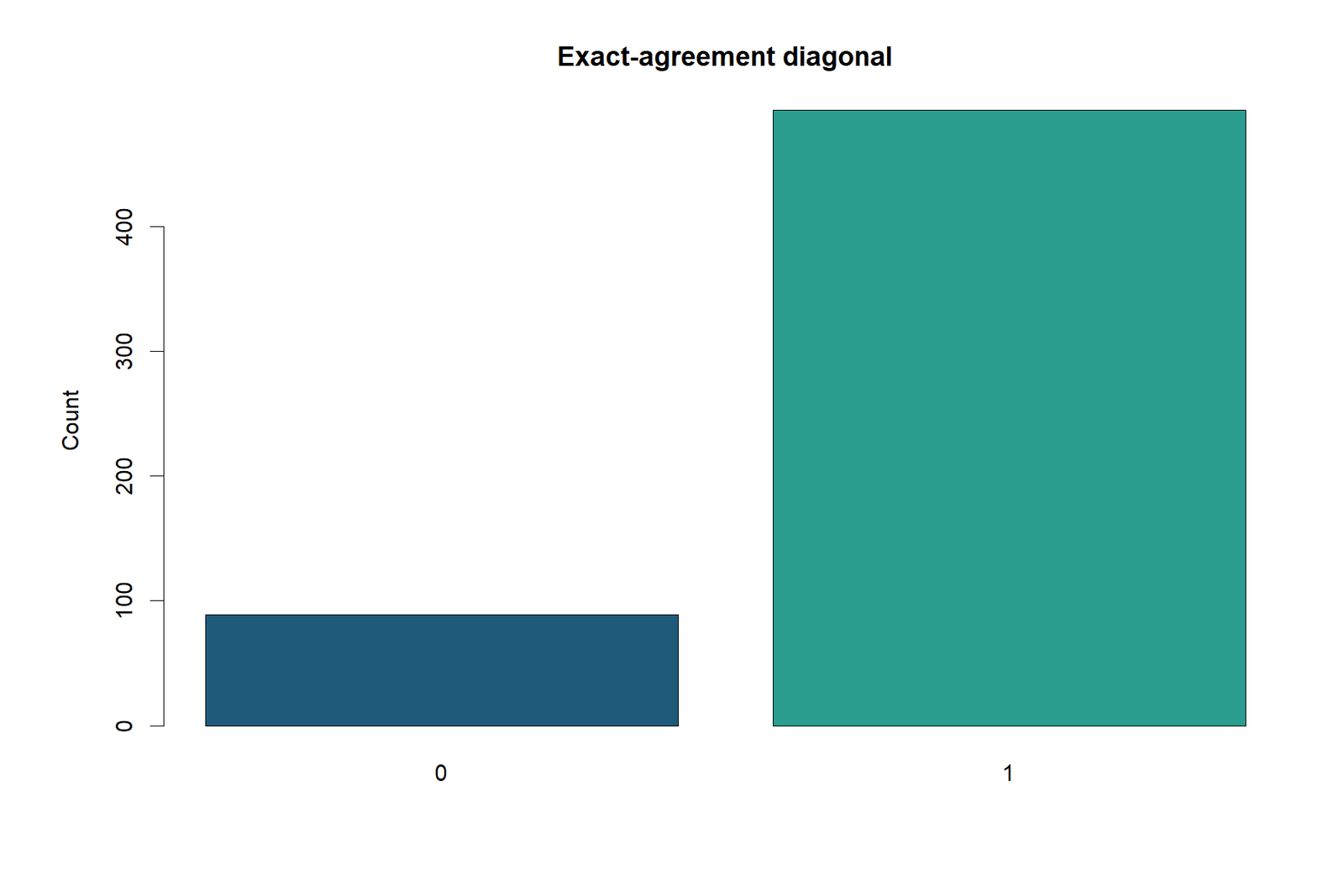
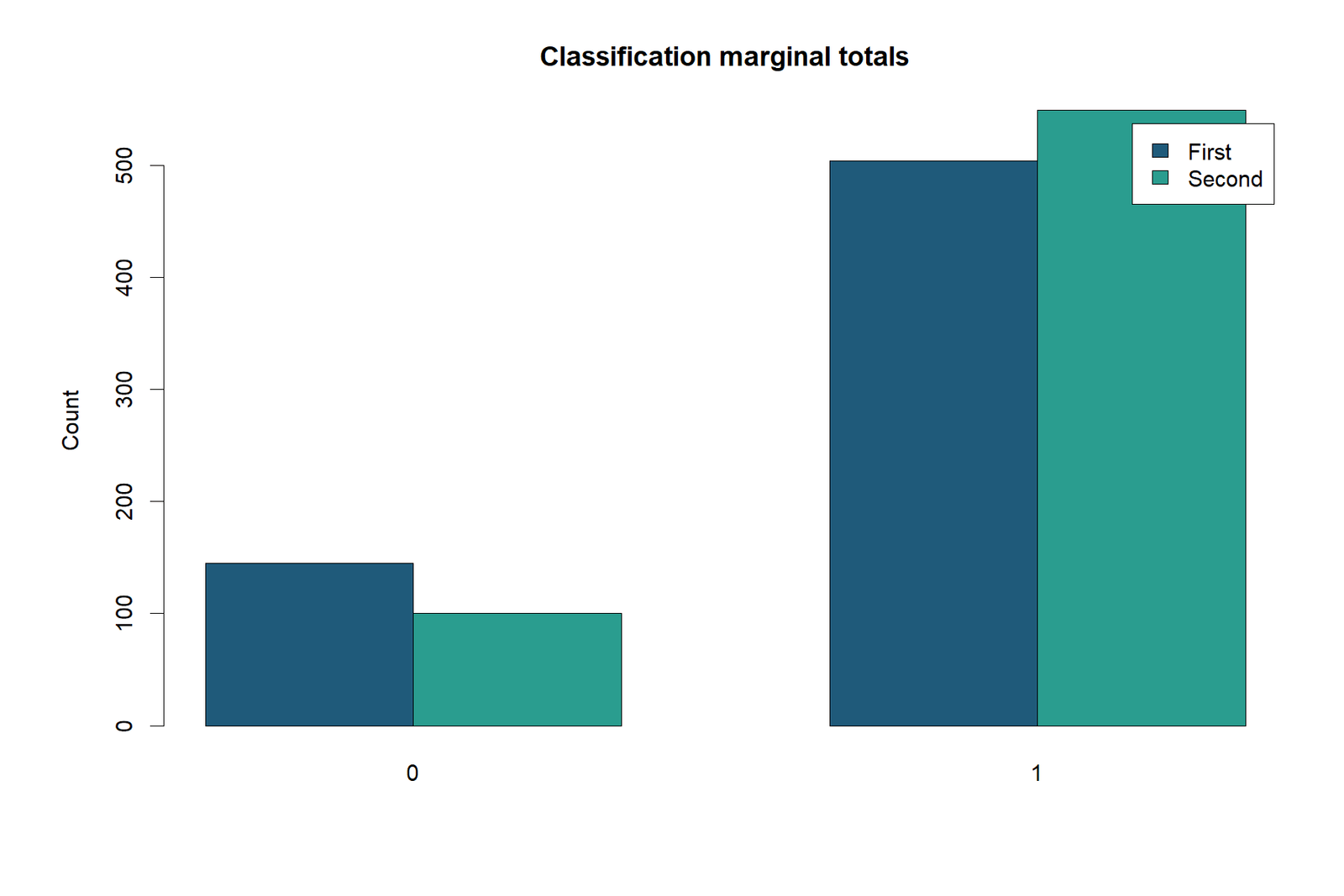
Pass agreement dominates the diagonal
The diagonal-count chart makes the category imbalance explicit. Most agreement comes from the pass category, not from a balanced combination of pass and fail agreements.
G3 classifies more students as passing
The G2 pass rate is 77.66%, while the G3 pass rate is 84.59%. The 6.93-point difference is the source of the binary bias index.
R pair 3: Observed versus expected agreement and result summary
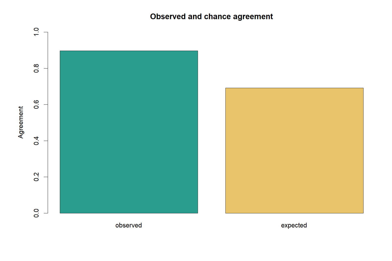
Observed agreement exceeds expectation by 20.54 points
The gap between 0.8968 observed agreement and 0.6913 expected agreement is the numerator of the agreement coefficient.
Strong but prevalence-sensitive agreement
The result summary shows κ = 0.6655 with a narrow interval and extremely small p-value. PABAK and category-specific agreement show that prevalence affects the conventional estimate.
Kappa Statistic in Python, R, SPSS, SAS and Excel
Kappa statistic in Python
Python can calculate κ from a confusion matrix or paired label vectors. A full workflow should also compute confidence intervals, PABAK, prevalence index, bias index and category-specific agreement. See categorical data analysis in Python and correlation in Python for related reproducible analysis patterns.
- Construct the 2 × 2 table.
- Verify category order.
- Calculate κ and its standard error.
- Calculate prevalence and bias diagnostics.
- Save tables, charts and report files.
Kappa statistic in R
R offers several agreement packages and manual matrix calculations. Always report the package, weighting choice and confidence-interval method because different functions can format or estimate uncertainty differently. See categorical data analysis in R.
- Use paired factors with identical levels.
- Request unweighted binary kappa.
- Inspect the agreement table and margins.
- Add positive and negative agreement manually.
- Export paired R charts and a PDF report.
Kappa statistic in SPSS
SPSS CROSSTABS can report Cohen's kappa for two categorical variables. The row and column category orders must match. Broader SPSS workflows are described in categorical data analysis in SPSS and correlation in SPSS.
- Place G2 binary in rows and G3 binary in columns.
- Request counts, row percentages and KAPPA.
- Confirm that 0 and 1 appear in the same order.
- Record κ, standard error and significance.
- Export SPV and PDF output.
Kappa statistic in Excel
Excel can reproduce the complete agreement coefficient calculation transparently. The supplied workbook contains data input, observed table, calculations, diagnostics and reporting sheets.
- Enter the four cell counts.
- Calculate row and column totals.
- Calculate Po and Pe from formulas.
- Calculate κ, PABAK, prevalence and bias indices.
- Audit all formulas against the verified reference values.
Kappa statistic in SAS
SAS PROC FREQ can generate agreement statistics for square contingency tables. Analysts should specify weights only for ordered categories and retain the unweighted analysis for nominal binary labels.
- Prepare paired classification variables.
- Use an agreement request in PROC FREQ.
- Confirm table ordering.
- Save ODS tables for reproducibility.
- Report κ with its standard error and confidence limits.
Expandable Code for the Kappa Statistic
Python code for the binary agreement coefficient
import numpy as np
from statsmodels.stats.inter_rater import cohens_kappa

table = np.array([[89, 56],
                  [11, 493]])
result = cohens_kappa(table)
print(result.kappa)
print(result.std_kappa)
print(result.kappa_low, result.kappa_upp)
print(result.pvalue_two_sided)

n = table.sum()
po = np.trace(table) / n
pabak = 2 * po - 1
prevalence_index = abs(table[0,0] - table[1,1]) / n
bias_index = abs(table[0,1] - table[1,0]) / n
R code for the binary agreement coefficient
tab <- matrix(c(89, 56, 11, 493), nrow = 2, byrow = TRUE)
n <- sum(tab)
po <- sum(diag(tab)) / n
row_p <- rowSums(tab) / n
col_p <- colSums(tab) / n
pe <- sum(row_p * col_p)
kappa <- (po - pe) / (1 - pe)
pabak <- 2 * po - 1
prevalence_index <- abs(tab[1,1] - tab[2,2]) / n
bias_index <- abs(tab[1,2] - tab[2,1]) / n
SPSS syntax for the agreement coefficient
CROSSTABS
 /TABLES=G2_PASS BY G3_PASS
 /FORMAT=AVALUE TABLES
 /STATISTICS=KAPPA
 /CELLS=COUNT ROW COLUMN TOTAL.
Excel formulas for the agreement coefficient
Observed agreement: =(B2+C3)/GrandTotal
Expected agreement: =(RowFail/GrandTotal)*(ColFail/GrandTotal)
                  +(RowPass/GrandTotal)*(ColPass/GrandTotal)
agreement coefficient: =(ObservedAgreement-ExpectedAgreement)/(1-ExpectedAgreement)
PABAK: =2*ObservedAgreement-1
Prevalence index: =ABS(B2-C3)/GrandTotal
Bias index: =ABS(C2-B3)/GrandTotal
SAS code for the Kappa Statistic
proc freq data=agreement_data;
  tables G2_PASS*G3_PASS / agree;
  exact kappa;
run;
Assumptions, Prevalence, Bias and Advanced Interpretation
Core assumptions
- Each subject is independent of other subjects.
- The two classifications are paired within subject.
- The category definitions are identical for both sources.
- Categories are mutually exclusive.
- The rating process is applied consistently.
- Missing classifications are handled transparently.
Important limitations
- Kappa depends on marginal prevalence.
- One coefficient can hide category-specific disagreement.
- Interpretive labels are conventions, not universal laws.
- Kappa does not identify which classifier is correct.
- A significant κ does not guarantee practical usefulness.
- Different weighting schemes can change ordinal results.
The prevalence paradox
A high percent agreement can coexist with a moderate or lower agreement coefficient when one category dominates. In this example, both sources classify most students as passing. That creates 69.13% expected agreement before any case-specific concordance is considered. The prevalence index of 0.6225 and PABAK of 0.7935 make this effect visible.
The bias effect
Bias refers to a difference between the marginal distributions of the two classification sources. G3 labels 84.59% as passing, compared with 77.66% for G2. The resulting bias index is 0.0693. Bias can either raise or lower κ depending on the table structure, so it should be interpreted together with prevalence rather than as an isolated defect.
Can the kappa statistic be negative?
Yes. A negative agreement coefficient means observed agreement is lower than expected from the margins. This can occur when raters systematically use opposite categories, when category coding is reversed or when a classification process is unstable. Always inspect the agreement matrix before interpreting a negative value.
Does a kappa statistic have a universal interpretation scale?
No. Terms such as slight, fair, moderate, substantial and almost perfect are descriptive conventions. Required reliability depends on the application. A screening tool, legal coding decision and exploratory classroom classification may need different minimum agreement. Confidence intervals, consequences and category-specific agreement should guide interpretation.
Sample size and statistical power
A narrow confidence interval requires enough paired cases and enough information across categories. When one category is rare, a large total sample may still provide imprecise negative agreement. Planning should consider expected prevalence, target κ, null κ, alpha and power. See statistical power, standard error and confidence interval.
APA Reporting for the Kappa Statistic
Complete worked-result template
Significant agreement
An unweighted agreement coefficient was calculated to assess agreement between G2 ≥ 10 and G3 ≥ 10 binary classifications for the same 649 students.
The classifications agreed for 582 of 649 cases (89.68%).
Agreement beyond chance was statistically significant, κ = .666, 95% CI [.593, .738], z = 17.40, p < .001.
Positive agreement was 93.64%, negative agreement was 72.65%, PABAK was .794, the prevalence index was .622 and the bias index was .069.
Use “substantial” only as a descriptive convention and retain the numerical estimate and interval.
Reusable agreement coefficient template
Fill-in format
A [weighted/unweighted] agreement coefficient was used to evaluate agreement between [classification source 1] and [classification source 2] for [N] paired cases.
Observed agreement was [Po or percentage], compared with expected agreement of [Pe].
The agreement coefficient was [κ], 95% CI [lower, upper], p = [p-value].
The result indicated [application-specific description] agreement beyond chance.
Add category-specific agreement and prevalence/bias diagnostics when the margins are imbalanced.
Non-significant or uncertain-result template
Use when applicable
The estimated agreement coefficient was [κ], 95% CI [lower, upper], p = [p-value].
The data did not provide clear evidence that agreement exceeded chance, and the confidence interval was compatible with [weak/zero/negative] agreement.
Observed agreement, expected agreement, marginal prevalence and sample size were considered before interpreting the coefficient.
For general reporting principles, see p-value, significance level and test statistic and effect size.
Common Kappa Statistic Mistakes and How to Correct Them
Common mistakes
- Reporting accuracy or percent agreement as the agreement coefficient.
- Using independent groups instead of paired classifications.
- Reversing category order for one classification source.
- Ignoring prevalence and bias effects.
- Using unweighted kappa for ordered multi-category data without justification.
- Calling a significant κ “perfect reliability.”
- Reporting only a conventional interpretation label.
- Failing to report the confusion matrix.
How to correct them
- Report Po, Pe and κ separately.
- Keep one paired row per case.
- Use identical category levels and order.
- Add PABAK, prevalence index and bias index.
- Declare whether weighting is used and why.
- Report confidence intervals and category-specific agreement.
- Interpret the coefficient in its application context.
- Publish the complete agreement table.
Mistaking high significance for high reliability
With large samples, even a small agreement coefficient can be statistically different from zero. Reliability should be judged from κ, its confidence interval, consequences of disagreement and category-specific performance—not from the p-value alone.
Using kappa to prove successful blinding
A agreement coefficient can describe agreement between perceived and actual assignments, but blinding success involves study design and interpretation beyond one coefficient. A non-significant κ does not prove perfect blinding, and a significant κ may reflect prevalence or systematic cues. The table and uncertainty must be examined directly.
Kappa Statistic Reports and Worked Excel Download
R PDF reportR analysis and paired chart interpretation for the same agreement table.
SPSS PDF outputSPSS kappa output for G2 and G3 binary classifications.
Worked Excel analysisData, agreement matrix, calculations, prevalence/bias diagnostics and reporting sheet.
Frequently Asked Questions About the Kappa Statistic
What is the agreement coefficient?
The agreement coefficient is a chance-corrected agreement coefficient for paired categorical classifications. It compares observed agreement with agreement expected from the marginal distributions.
How do you calculate the agreement coefficient?
Calculate observed agreement, calculate expected agreement from row and column margins, then use κ = (Po − Pe)/(1 − Pe).
What does a agreement coefficient of 0.67 mean?
It indicates strong agreement beyond chance in many common interpretation systems, but the confidence interval, prevalence, bias and application requirements should determine the final wording.
Why is kappa lower than percent agreement?
Percent agreement does not remove agreement expected from marginal prevalence. When one category is common, expected agreement can be high and conventional kappa can be much lower than raw agreement.
Can a agreement coefficient be negative?
Yes. Negative kappa means the observed agreement is lower than the chance expectation calculated from the margins.
Is the agreement coefficient an effect size?
It is a standardized agreement coefficient, but its interpretation is influenced by category prevalence and bias. It should be accompanied by the agreement matrix and confidence interval.
What is PABAK?
PABAK is prevalence-adjusted bias-adjusted kappa, calculated as 2Po − 1. It is a sensitivity diagnostic, not an automatically superior replacement for conventional kappa.
What is the prevalence index?
For a binary table, the prevalence index summarizes imbalance between the two diagonal agreement cells. A high value indicates that agreement is concentrated in one category.
What is the bias index?
The bias index summarizes imbalance between the two off-diagonal disagreement cells and therefore differences in the marginal classification rates.
What is positive agreement?
Positive agreement is category-specific concordance for the positive category. In this example, agreement on passing is 93.64%.
What is negative agreement?
Negative agreement is category-specific concordance for the negative category. In this example, agreement on failing is 72.65%.
When should weighted kappa be used?
Use weighted kappa for ordered categories when adjacent disagreements should be penalized less than extreme disagreements.
When should Fleiss kappa be used?
Use a Fleiss-type kappa when multiple raters classify the same items into nominal categories and one common multi-rater agreement coefficient is required.
Is kappa the same as ICC?
No. Kappa is mainly for categorical classifications. ICC is designed for numerical ratings or measurements and depends on a chosen reliability model.
How should the agreement coefficient be reported?
Report the paired variables, sample size, agreement matrix or percent agreement, κ, confidence interval, p-value and relevant prevalence/bias or category-specific diagnostics.
Kappa Statistic Conclusion
The agreement coefficient provides a more informative agreement assessment than percent agreement alone because it accounts for the agreement expected from the category margins. In this worked example, G2 and G3 pass/fail classifications agreed for 89.68% of 649 students. Expected agreement was already 69.13%, producing κ = 0.6655, 95% CI [0.5927, 0.7384], p < .001.
The classifications therefore demonstrate strong agreement beyond chance, but the complete diagnostic picture is more nuanced. Passing is common, PABAK is 0.7935, the prevalence index is 0.6225, and positive agreement is substantially higher than negative agreement. The most defensible conclusion is not merely “kappa was substantial.” It is that the two classifications agree strongly overall, agreement is concentrated in the pass category, and marginal prevalence materially affects the conventional agreement coefficient.
For the next steps, review effect size, confidence interval, correlation versus regression and chi-square assumptions to distinguish agreement, association, prediction and uncertainty clearly.

