
Cronbach’s Alpha: Formula, Interpretation, Good Values, SPSS, Python, R and Excel
Cronbach’s Alpha is one of the most widely reported measures of internal consistency, but it is also one of the most frequently misunderstood. This guide explains what Cronbach’s Alpha measures, its symbol and formula, what counts as a good value, raw versus standardized alpha, assumptions, negative alpha, alpha if item deleted, corrected item-total correlations, SPSS output, Python, R and Excel calculations, APA reporting, ten chart interpretations and a complete 649-case worked example.
The worked six-item scale has poor internal consistency
The verified result is Cronbach’s Alpha = 0.111763 for 649 complete cases and six transformed items. The standardized coefficient is 0.168910. These values are far below commonly used screening levels such as 0.70. The result does not mean that the software failed. It means that the six variables do not share enough positive covariance to support a dependable single raw-score composite.
The item matrix explains the low value. Inter-item correlations range from -0.389 to 0.617, and the average inter-item correlation is only 0.032763. Several item pairs move in opposite directions. Deleting goout raises alpha to 0.234087, but that remains low. The defensible conclusion is to review the construct, scoring and dimensionality rather than delete one item and declare the scale reliable.
Verified metrics
Contents
What Is Cronbach’s Alpha?
Cronbach’s Alpha summarizes the internal consistency of a set of scored items intended to contribute to one composite.
Cronbach’s Alpha, often called coefficient alpha, is a statistic calculated from the variances and covariances of multiple items. It estimates how consistently the items contribute to a shared score under a specific measurement model. The coefficient is usually represented by the Greek letter alpha, α, and ranges upward toward 1 when the items have stronger positive relationships. Values can be zero or negative when the average covariance is weak or opposite in direction.
The phrase internal consistency describes the degree to which responses to items move together within one administration. It does not automatically mean that the instrument is stable over time, that different raters agree, or that the scale measures the intended construct. A test-retest design addresses temporal stability, while intraclass correlation coefficient guide or categorical agreement methods such as Cohen's Kappa guide answer different reliability questions. Cronbach’s Alpha is specifically about the covariance structure among items used to build a composite score.
Cronbach’s Alpha became popular because it can be calculated from a single administration and is available in nearly every statistical package. Its convenience should not be confused with completeness. A high value does not prove unidimensionality or validity, and a low value does not identify the exact cause. The coefficient must be interpreted with item content, scoring direction, the inter-item matrix, corrected item-total correlations and the intended use of the score.
In the worked analysis, six transformed variables are combined: family relationship quality, free time, going out with friends, reverse-scored weekday alcohol use, reverse-scored weekend alcohol use and health. The verified Cronbach’s Alpha is 0.111763. That very low value is understandable because the item set mixes several substantive domains and includes both positive and negative inter-item relationships.
The descriptive statistics guide and standard deviation guide should be reviewed before alpha because internal-consistency calculations depend on item variances and total-score variance. A data error, constant item, restricted response range or incorrect reverse scoring can materially change the coefficient. A professional reliability analysis therefore begins with data and scoring checks rather than clicking a software menu first.
What Does Cronbach’s Alpha Measure?
The coefficient reflects shared covariance among the scored items, not every possible meaning of reliability.
Cronbach’s Alpha measures the extent to which a set of item scores has a common covariance pattern that supports combining them into one score. When respondents who score high on one item also tend to score high on the others, total-score variance becomes large relative to the sum of individual item variances, and alpha increases. When the items are unrelated or some move in opposite directions, the coefficient decreases.
The coefficient is influenced by two broad factors: the average relationship among items and the number of items. Adding items that are positively related to the existing scale can raise alpha even when the average relationship stays modest. This is why a long questionnaire may show a high coefficient despite substantial redundancy or multiple closely related dimensions. Conversely, a short scale may have a moderate alpha even when its items are reasonably coherent.
Cronbach’s Alpha does not directly measure item quality, construct validity, predictive accuracy, rater agreement or stability across time. It also does not prove that every item measures exactly the same latent variable. A multidimensional scale can produce a respectable coefficient when its dimensions are correlated or when the scale is long. Factor analysis, theoretical review and external validation are needed to justify the meaning of the score.
For the six-item example, average inter-item correlation is only 0.032763. The item pairs range from -0.389 to 0.617. The strong positive relationship between the two reverse-scored alcohol-use variables is offset by negative relationships between social activity and the reverse-scored alcohol variables. Cronbach’s Alpha correctly compresses this mixed covariance structure into a low overall coefficient, but the matrix is required to understand why.
When users ask whether Cronbach’s Alpha measures reliability, the precise answer is that it is an internal-consistency coefficient under assumptions about the score model. Reliability is broader than internal consistency. A scale could have high alpha but poor test-retest stability, or low alpha because it intentionally forms a broad index from components that need not correlate. The intended measurement model determines whether alpha is appropriate.
Cronbach’s Alpha Formula, Equation and Symbol
The raw-score formula compares the sum of item variances with the variance of the total score.
The symbol for Cronbach’s Alpha is the Greek letter α. Let k be the number of items, sj2 the sample variance of item j, and sT2 the variance of the summed total score. The standard raw-score equation is shown below.
The coefficient rises when the total score contains more shared covariance relative to separate item variance.
The total-score variance contains every item variance plus twice every unique item covariance. When covariances are positive, the variance of the sum becomes larger than the sum of the separate variances, which raises Cronbach’s Alpha. Negative covariances work in the opposite direction. This variance identity explains why correct scoring direction is essential. A reversed item left uncorrected can reduce total-score variance and produce a low or negative alpha.
For the worked data, there are six items, the sum of item variances is approximately 7.997, and the total-score variance is 8.818553. Substituting these values into the equation produces 0.111763. Python, R, SPSS and Excel agree to floating-point precision. The workbook calculation differs from the verified reference by less than two quadrillionths, demonstrating that the result is computationally stable.
An alternative standardized formula uses the average inter-item correlation, r̄. It is useful when items have different variances or units and the analyst wants the coefficient based on a correlation matrix.
With k = 6 and average inter-item r = 0.032763, standardized alpha equals 0.168910.
The formula should be reported with enough precision to reproduce the calculation, but the published coefficient is normally rounded to two or three decimals. Report α = .112 rather than a long string unless a technical appendix requires exact values. The variance guide explains the variance component that drives the raw-score equation.
What Is a Good Cronbach’s Alpha Value?
Common thresholds are context-dependent screening conventions rather than universal pass-or-fail laws.
A commonly quoted interpretation treats Cronbach’s Alpha values of .70 or higher as acceptable for preliminary group-level research, .80 or higher as good, and .90 or higher as excellent. Values below .60 are often described as poor. These labels are convenient, but they should not be treated as immutable scientific boundaries. The acceptable level depends on the stakes, construct breadth, scale length, measurement purpose and consequences of error.
| Alpha range | Common descriptive label | Practical interpretation |
|---|---|---|
| Below .50 | Very poor | The item set has little shared covariance; check coding and scale definition. |
| .50 to .59 | Poor | Usually insufficient for a dependable composite. |
| .60 to .69 | Questionable | May be tolerated in early exploratory work with strong justification. |
| .70 to .79 | Acceptable | Common group-research screening range, subject to assumptions. |
| .80 to .89 | Good | Stronger consistency for many research applications. |
| .90 to .95 | Very high | May suit high-stakes use but requires validation and precision evidence. |
| Above .95 | Possible redundancy | Items may be overly repetitive or narrowly worded. |
The threshold should be more demanding when individual decisions are made, when score differences have serious consequences, or when a narrow construct is expected. Exploratory research, newly developed scales or broad constructs may temporarily accept lower values while the item pool is revised. Reporting a threshold without the context creates false certainty.
A very high Cronbach’s Alpha is not automatically superior. Values above .95 can indicate that multiple items ask nearly the same question. Redundancy may increase alpha while narrowing content coverage and burdening respondents. The aim is not to maximize the coefficient at any cost; the aim is to produce a score that is coherent, valid, efficient and appropriate for its intended use.
The worked result of .111763 is far below every common screening level. Standardized alpha of .168910 does not change the conclusion. The coefficient is not borderline, and sampling noise is not a plausible explanation for such a large deficit with 649 complete cases. The item set should be reconsidered before its total score is used as a reliability-supported scale.
Alpha thresholds should be interpreted alongside confidence intervals and evidence about dimensionality. A narrow confidence interval around .55 still indicates inadequate consistency, while a broad interval around .75 signals uncertainty. The confidence interval guide provides the general logic for reporting estimate precision.
Worked Cronbach’s Alpha Variables, Coding and Data Structure
The example uses six 1-to-5 items after reverse scoring weekday and weekend alcohol use.
The verified analysis includes 649 complete rows and six variables. Family relationship quality, free time, going out and health are used in their original 1-to-5 direction. Weekday and weekend alcohol-use values are transformed with 6 - original score, so higher values represent lower alcohol use. The transformation aligns the intended direction before Cronbach’s Alpha is calculated.
| Item | Meaning | Coding | Mean | SD |
|---|---|---|---|---|
| famrel | Quality of family relationships | 1 to 5; higher = better | 3.9307 | 0.9557 |
| freetime | Free time after school | 1 to 5; higher = more | 3.1803 | 1.0511 |
| goout | Going out with friends | 1 to 5; higher = more | 3.1849 | 1.1758 |
| Dalc_R | Reverse-scored weekday alcohol use | 6 – Dalc; higher = lower use | 4.4977 | 0.9248 |
| Walc_R | Reverse-scored weekend alcohol use | 6 – Walc; higher = lower use | 3.7196 | 1.2844 |
| health | Self-reported health | 1 to 5; higher = better | 3.5362 | 1.4463 |
All six items share the same nominal range after transformation, but equal ranges do not mean that they form one construct. Family relationships, leisure, social activity, alcohol use and health are conceptually diverse. This is a useful demonstration of why Cronbach’s Alpha should evaluate a theoretically defined scale rather than convert unrelated variables into a scale simply because they can be summed.
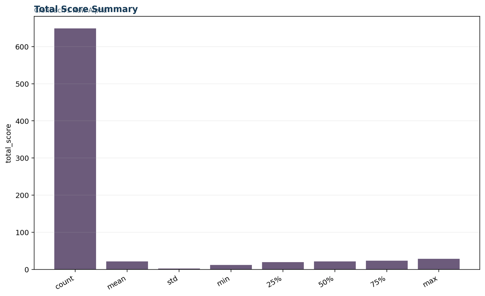
There are no missing values among the six variables in the worked dataset, so SPSS uses listwise N = 649. The total score ranges from 12 to 29, with mean 22.0493, median 22 and standard deviation 2.9696. Before calculating alpha in another dataset, document missing-data rules because listwise deletion, pairwise covariance and person-mean imputation can produce different coefficients.
Item distributions should be checked with frequency and relative frequency tables and descriptive summaries. A ceiling effect can restrict covariance, and an impossible value can distort the total score. In this dataset, reverse-scored weekday alcohol use has the highest mean and smallest standard deviation, suggesting concentration toward lower reported use. That restriction may affect relationships, although the larger issue is the heterogeneous content of the item set.
Complete Cronbach’s Alpha Worked Result
The overall coefficient, standardized coefficient, total-score distribution and item diagnostics all indicate poor consistency.
The raw Cronbach’s Alpha coefficient is 0.1117626312468654, which is reported as α = .112. Standardized alpha is 0.1689095701610637. The total-score variance is 8.818552759230725, and the average inter-item correlation is 0.0327632892853925. These values are independently reproduced by Python, R, SPSS and Excel.
| Metric | Exact value | Rounded report value | Interpretation |
|---|---|---|---|
| Valid cases | 649 | 649 | All records complete for six items |
| Number of items | 6 | 6 | Short six-item composite |
| Raw Cronbach alpha | 0.1117626312468654 | .112 | Very poor internal consistency |
| Standardized alpha | 0.1689095701610637 | .169 | Still very poor |
| Average inter-item correlation | 0.0327632892853925 | .033 | Items barely move together on average |
| Total-score variance | 8.818552759230725 | 8.819 | Variance used in raw-alpha formula |
| Total-score mean | 22.0493066255778 | 22.049 | Center of summed score |
| Total-score SD | 2.96960481532993 | 2.970 | Spread of summed score |
The difference between raw and standardized alpha is modest. Standardization increases the value because the item standard deviations differ, but the weak correlation pattern remains. Standardizing cannot create a common construct where item relationships are inconsistent. It simply gives each item equal variance before calculating the coefficient.
The total-score distribution appears reasonably concentrated around 22 to 24, with minimum 12 and maximum 29. A smooth total-score histogram does not prove reliability. A composite can look statistically well behaved while its components fail to measure one coherent attribute. Cronbach’s Alpha depends on covariance, not on the visual normality of the sum.
The strongest corrected item-total correlation is 0.226597 for famrel, while the weakest is -0.104770 for goout. None reaches the common .30 item-rest benchmark. Deleting goout produces the highest alpha-if-deleted value, .234087, but this remains inadequate. The result therefore supports redesigning the scale rather than making one isolated deletion.
Variance, Covariance and Inter-Item Components of Cronbach’s Alpha
The low coefficient is generated by a mixture of strong positive, weak and negative pairwise relationships.
The raw Cronbach’s Alpha formula is easiest to understand through the item covariance matrix. Positive covariance means that two items tend to rise together. Negative covariance means that high scores on one tend to accompany low scores on the other. The worked matrix contains values from -0.587 to 0.732. Average inter-item covariance is only about 0.027, which is small relative to average item variance of approximately 1.333.
| Pair | Correlation | Covariance | Interpretive note |
|---|---|---|---|
| Dalc_R with Walc_R | .617 | .732 | Strong positive relationship between reverse-scored alcohol-use items |
| freetime with goout | .346 | .428 | Moderate leisure and social-activity relationship |
| goout with Walc_R | -.389 | -.587 | Strongest negative pair in the scale |
| goout with Dalc_R | -.245 | -.267 | Social activity opposes lower weekday alcohol use |
| Walc_R with health | -.115 | -.214 | Small negative relationship |
| famrel with health | .110 | .151 | Small positive relationship |
The strongest positive pair is the two reverse-scored alcohol-use items. That relationship by itself would support a small alcohol-use subscale, but it does not make the six-item total coherent. The social variables correlate positively with each other but negatively with the alcohol variables. This opposing structure reduces total-score variance relative to separate item variances and lowers Cronbach’s Alpha.
Average inter-item correlation is often useful because it is less dependent on the number of items than alpha. For a broad construct, a moderate average correlation may be reasonable, whereas a narrow scale should show stronger relationships. An average of .033 is too close to zero to support a common reflective scale. The range from -.389 to .617 also signals that the average hides meaningful subgroups.
The covariance and correlation matrices should be inspected before any item is deleted. If the matrix reveals clusters, factor analysis or subscale development may be more appropriate than forcing one total. The correlation assumptions guide explains the linear-association assumptions behind Pearson correlations used in the matrix.
Raw Versus Standardized Cronbach’s Alpha
Raw alpha uses the covariance matrix; standardized alpha uses the correlation matrix.
Raw Cronbach’s Alpha preserves the original item variances and is appropriate when items share a meaningful unit and the raw sum is the intended score. Standardized alpha first converts items to equal variance and is calculated from their correlation matrix. It is useful when item scales or variances differ and the analyst wants to remove scale-unit effects.
In the worked example, every item uses a 1-to-5 range, but their variances still differ. Health has variance about 2.092, whereas reverse-scored weekday alcohol use has variance about 0.855. Standardization gives these items equal variance, raising alpha from .112 to .169. The increase shows that variance differences suppress the raw coefficient slightly, but the standardized result remains very poor because the average correlation is weak.
Analysts should report the coefficient that matches the score actually used. If respondents receive a raw summed score, raw alpha is normally primary. If items are standardized before forming the composite, standardized alpha may be more relevant. Reporting standardized alpha to make a weak raw result appear stronger is not defensible. Both may be shown when their difference is substantively informative.
The two versions answer slightly different questions but share the same limitations. Neither proves unidimensionality, and neither compensates for mixed item direction or multidimensionality. If standardized alpha is much higher than raw alpha, investigate differences in variance, response ranges and item weighting. The standard deviation guide and variance guide provide the descriptive foundations for this comparison.
For this dataset, both versions lead to the same decision. Cronbach’s Alpha is too low to support the proposed total. The gap between .112 and .169 is not large enough to alter interpretation, and the correlation matrix provides direct evidence that conceptual heterogeneity is the dominant problem.
Cronbach’s Alpha If Item Deleted
The deletion column identifies which item changes consistency, but it does not decide content validity.
Cronbach’s Alpha if item deleted recalculates the coefficient after removing one item. It helps identify items that contribute negative covariance or weak alignment. A deleted-item alpha above the original coefficient means the remaining set is more internally consistent. A lower value means the removed item was supporting the covariance structure.
| Deleted item | Alpha if deleted | Change from .111763 | Interpretation |
|---|---|---|---|
| famrel | -0.056486 | -0.168248 | Remaining items have negative average covariance |
| freetime | -0.002364 | -0.114127 | Removal worsens the covariance structure |
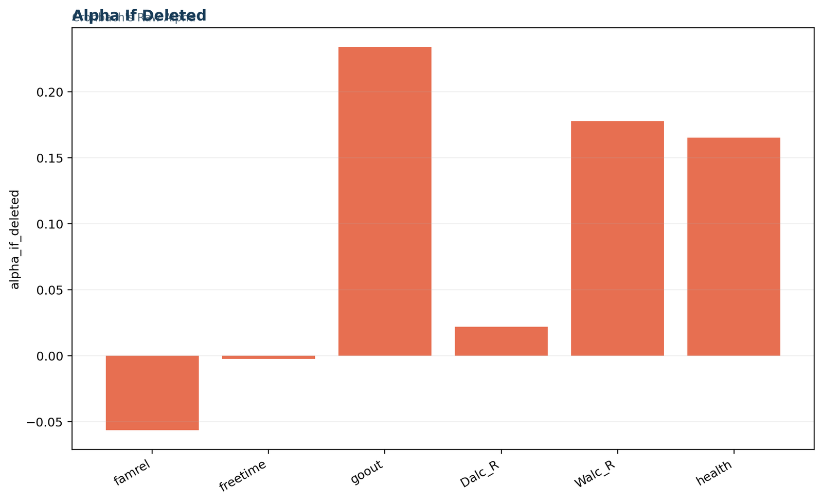
| goout | 0.234087 | +0.122325 | Largest improvement, but still poor |
| Dalc_R | 0.021909 | -0.089854 | Removal reduces consistency |
| Walc_R | 0.177823 | +0.066060 | Some improvement, still poor |
| health | 0.165338 | +0.053575 | Some improvement, still poor |
Deleting goout produces the largest increase because it has negative relationships with both reverse-scored alcohol items. Deleting Walc_R or health also raises alpha modestly. However, none of the reduced scales approaches .70. A mechanical delete-the-worst strategy would therefore fail to solve the underlying measurement problem.
Negative alpha-if-deleted values for famrel and freetime occur because the remaining items have negative average covariance. SPSS flags this and recommends checking item coding. The warning is appropriate, but coding is not the only possibility. The retained items may simply represent incompatible constructs.
Item deletion changes what the score measures. A theoretically essential item should not be discarded solely to raise Cronbach’s Alpha, and a redundant item should not be retained solely because it raises alpha. Use the deletion table with content review, factor analysis, respondent feedback and the corrected item-total correlation guide. A transparent decision log should state whether an item was retained, revised, moved to a subscale or removed and why.
Corrected Item-Total Correlation and Cronbach’s Alpha
Item-rest coefficients localize the item-level relationships behind the overall reliability value.
The corrected item-total correlation is the correlation between an item and the total of the remaining items. It avoids the inflated part-whole relationship created when the item is included in its own total. The coefficient is a direct item-level companion to Cronbach’s Alpha. Positive values indicate alignment with the rest score, while negative values signal opposite direction.
| Item | Corrected item-total r | Common .30 screen | Alpha if deleted |
|---|---|---|---|
| famrel | 0.226597 | Below | -0.056486 |
| freetime | 0.151318 | Below | -0.002364 |
| goout | -0.104770 | Negative | 0.234087 |
| Dalc_R | 0.139144 | Below | 0.021909 |
| Walc_R | -0.033120 | Negative | 0.177823 |
| health | -0.010454 | Negative | 0.165338 |
None of the six coefficients reaches .30, and three are negative. The pattern is consistent with the low alpha and confirms that the weakness is not caused by one isolated item. The strongest item, famrel, still has only a modest association with the rest score. The weakest item, goout, moves in the opposite direction.
Corrected item-total coefficients should be interpreted with item variance and content. A low value can reflect restricted range, ambiguous wording, a different subdimension or an item that is necessary but unique. A high value can reflect desirable consistency or redundancy. The dedicated corrected item-total correlation guide provides a full formula, cutoff, SPSS, Python, R and Excel explanation.
When Cronbach’s Alpha is low, the item-rest table helps determine whether the problem is global or local. A single negative item amid otherwise strong coefficients suggests a coding or wording issue. Many weak coefficients, as seen here, suggest that the total score itself is not well defined. This distinction guides whether the next action is a targeted correction or a complete scale redesign.
Cronbach’s Alpha Assumptions and Limitations
Meaningful interpretation requires a coherent scale, appropriate scoring, independent errors and a justified measurement model.
The first requirement for Cronbach’s Alpha is that the items are intended to contribute to a common reflective construct. Alpha is not an appropriate quality target for a formative index whose components define a score but need not correlate. Combining income, education and housing conditions into an index, for example, does not require those components to behave like interchangeable indicators.
A strict reliability interpretation assumes essential tau-equivalence: items measure the same underlying construct with equal true-score loadings, allowing different constants and error variances. When loadings differ substantially, alpha can understate or overstate reliability. Congeneric measures such as omega are often more flexible because they allow different factor loadings. Alpha remains useful as a descriptive internal-consistency coefficient when its assumptions and limits are acknowledged.
Errors should be uncorrelated after accounting for the common score. Similar wording, shared item stems, reverse-wording method effects or repeated content can create correlated errors and inflate Cronbach’s Alpha. Conversely, poorly worded reverse items can introduce method variance and reduce the coefficient. Inspect residual relationships and factor structure when the score has important consequences.
Items must be scored in the same conceptual direction. Reverse-scored variables should be transformed before calculation. In the worked data, Dalc and Walc are reversed as 6 - score. Even after correct reversal, alpha remains low, demonstrating that direction correction is necessary but not sufficient.
Rows should be independent for conventional precision estimates. Repeated observations, clustered classrooms or duplicate respondents require a design-aware approach. Missing data must be handled consistently, and item distributions should be inspected for floor, ceiling and impossible values. The outlier detection guide and frequency and relative frequency tables support these data-quality checks.
Alpha does not require a normally distributed total to be computed, but normal-theory confidence intervals may be affected by nonnormality, ordinal categories and small samples. Bootstrap intervals or ordinal methods may be preferable. The Shapiro-Wilk test guide should not be used as a mechanical prerequisite for Likert-scale alpha; distributional assessment should focus on the purpose and estimator.
Negative, Zero and Extremely High Cronbach’s Alpha
Unusual values are diagnostic signals that require coding, content and covariance review.
A negative Cronbach’s Alpha means the sum of item variances exceeds the variance of the total score after the formula adjustment. This occurs when average covariance is negative. The most common cause is an item scored in the opposite direction, but negative alpha can also arise from combining unrelated or inversely related constructs. It should never be interpreted as simply “reliability below zero” without investigation.
An alpha near zero indicates that the items share almost no average covariance. The worked value of .112 is positive but close enough to zero to signal very weak consistency. With a short scale, sampling variability can be substantial, yet a coefficient this low in 649 cases is not a minor fluctuation. The item matrix clearly supports the conclusion.
An extremely high value, especially above .95, may indicate item redundancy. Several items may restate the same idea with minor wording changes. Redundancy increases respondent burden and narrows content without necessarily improving validity. Check inter-item correlations for values approaching 1 and review whether each item adds meaningful information.
Alpha can also exceed 1 in erroneous calculations caused by an invalid covariance matrix, inconsistent missing-data treatment or formula mistakes. A correctly calculated coefficient from a valid covariance matrix should not exceed 1. Software output outside the expected range should trigger a complete data and computation audit.
When an unusual Cronbach’s Alpha appears, follow a fixed sequence: verify data ranges, confirm reverse scoring, inspect item variances, inspect covariance signs, review corrected item-total correlations, examine dimensionality and replicate the result in another program. The cross-software agreement in this worked example confirms that the low value is a property of the item set rather than a software error.
Cronbach’s Alpha Python Charts
The Python figures visualize the raw coefficient, variance components, deletion effects, score distribution and verified summary.
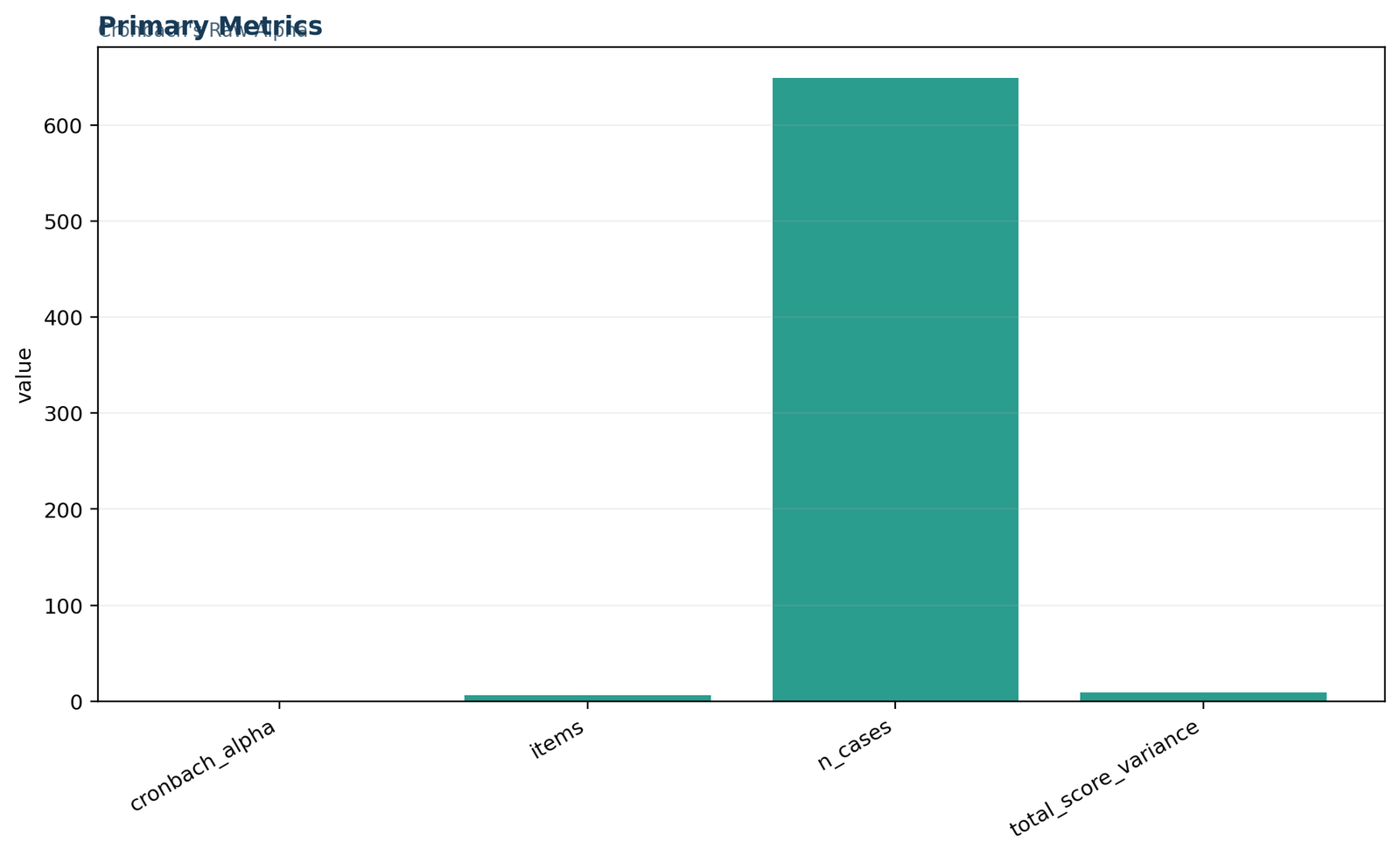
The Python chart set turns the Cronbach’s Alpha calculation into a visual audit. Figure 1 presents the principal values: raw alpha, number of items, number of cases and total-score variance. The small raw coefficient stands out immediately against the other scale metrics and prevents a reader from mistaking sample size for measurement quality.
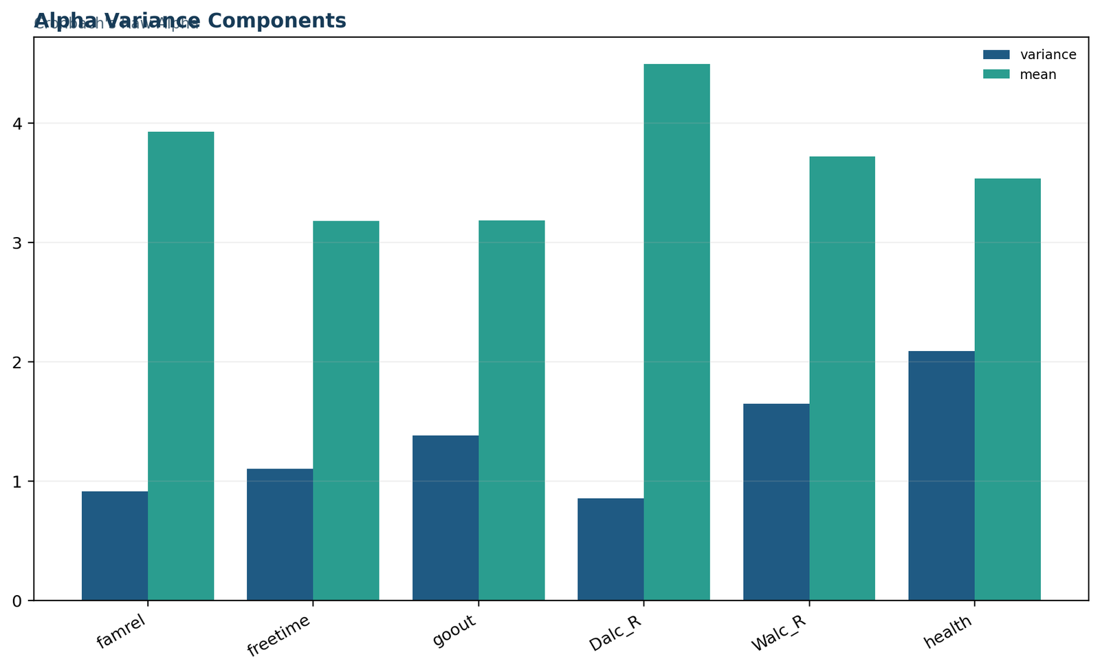
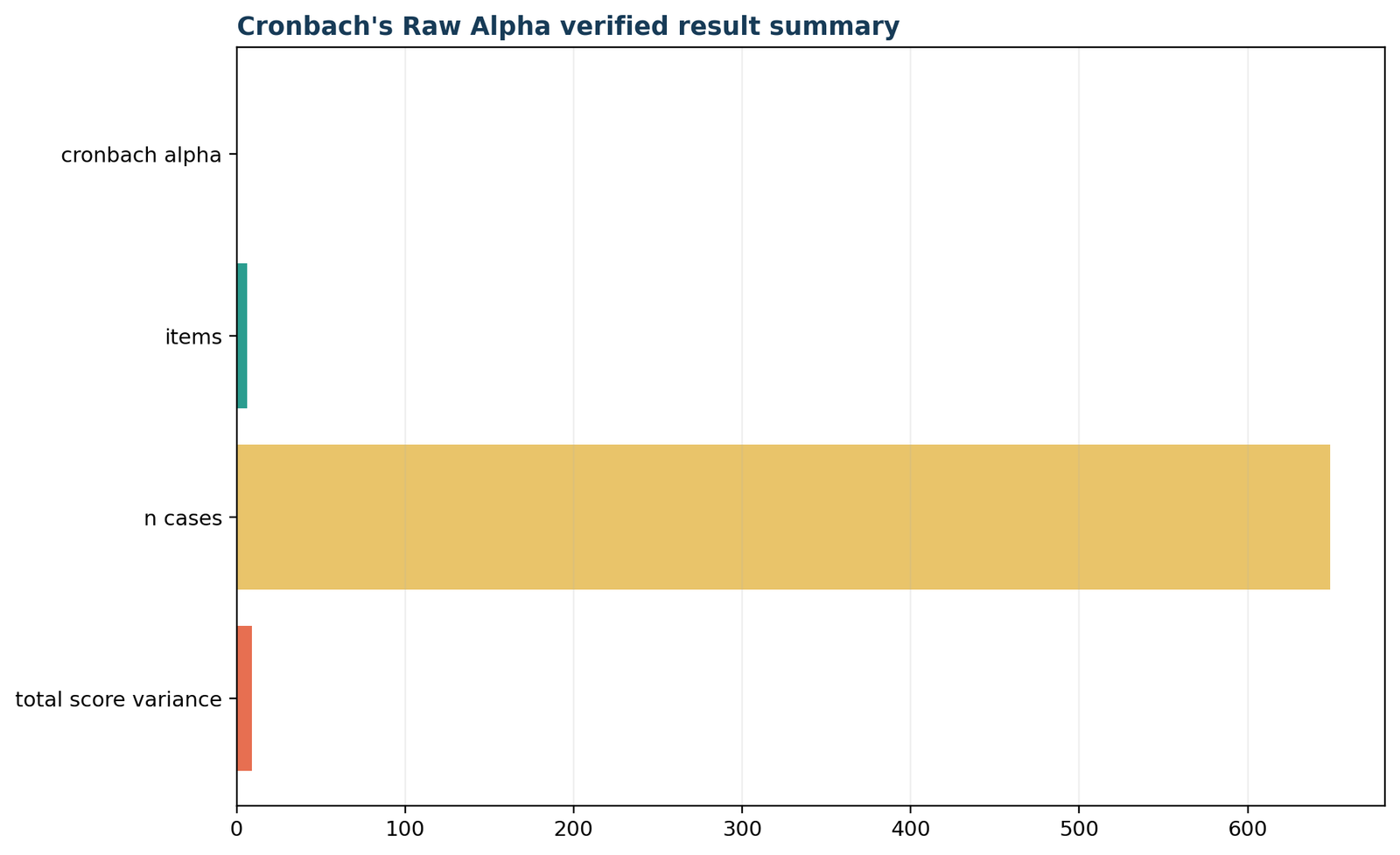
Python Figure 2 displays the variance components used in the formula. The total-score variance is only slightly larger than the sum of item variances because positive and negative covariances offset each other. This is the numerical reason raw alpha remains low. The figure should be read with the covariance matrix rather than interpreted as an isolated bar comparison.
Python Figure 3 compares alpha if each item is deleted. Removing goout produces the highest remaining coefficient, approximately .234. Removing Walc_R or health gives smaller improvements. The negative values after deleting famrel or freetime reflect negative average covariance in the reduced set.
Python Figure 4 summarizes the total score. The mean is 22.0493, the median is 22, the standard deviation is 2.9696 and observed values range from 12 to 29. The distribution is useful for describing the score but cannot rescue poor internal consistency. A total can be approximately bell shaped even when its items do not form a coherent scale.
Python Figure 5 confirms the independently verified metrics and cross-check status. The Python analysis reproduces the same raw alpha and total-score variance as R, SPSS and Excel. Readers who need the underlying correlation workflow can use the correlation in Python guide.
Cronbach’s Alpha R Charts
The R implementation independently confirms every primary coefficient and item-deletion pattern.
The R figures are interpreted separately because independent software agreement is part of the quality evidence. R reconstructs the six scored items, calculates the covariance matrix, total-score variance, raw Cronbach’s Alpha and alpha after deleting each item. The resulting metrics match Python and the SPSS reliability procedure.
R Figure 1 confirms raw alpha of 0.111763, six items and 649 cases. R Figure 2 reproduces the formula components and shows why the total variance is insufficient relative to separate item variances. R Figure 3 confirms that goout is the deletion that gives the largest increase, although the reduced coefficient is still poor.
R Figure 4 describes the total-score distribution, while R Figure 5 consolidates the final values and verification status. The complete match across programs indicates that rounding and software defaults are not changing the substantive conclusion.
R users should calculate covariance with a consistent complete-case rule and avoid silently switching to pairwise deletion. The correlation in R guide explains correlation functions that support matrix diagnostics. Packages that report omega or ordinal alpha can be added when the measurement model requires a more flexible estimator.
The R chart evidence supports the same interpretation as Python: Cronbach’s Alpha is very low because the proposed score combines weakly related and oppositely related items. The next step is conceptual and psychometric revision, not a different plotting package.
How to Calculate and Interpret Cronbach’s Alpha in SPSS
SPSS Reliability Analysis provides alpha, standardized alpha, item-total statistics and covariance diagnostics.
In SPSS, choose Analyze → Scale → Reliability Analysis. Move the scored items into the Items box and select Model = Alpha. In Statistics, request item, scale, scale if item deleted, correlations and covariances. The output begins with Case Processing Summary and Reliability Statistics, followed by Item Statistics, correlation and covariance matrices, Item-Total Statistics and Scale Statistics.
The worked SPSS output reports 649 valid cases, zero excluded cases, raw Cronbach’s Alpha = .112, standardized alpha = .169 and six items. The result is rounded in the visible table, while the verification section records full precision of 0.1117626312468654. Report α = .112 rather than copying the software value as .000-style significance notation.
The Item-Total Statistics table is central to interpretation. It reports corrected item-total correlation, squared multiple correlation and alpha if item deleted. The goout row has corrected r = -.105 and alpha if deleted = .234. The output warns that negative alpha-if-deleted values arise from negative average covariance and recommends checking item codings.
The Inter-Item Correlation Matrix shows the strongest positive pair, Dalc_R with Walc_R at .617, and the strongest negative pair, goout with Walc_R at -.389. The correlation in SPSS guide explains SPSS correlation matrices, two-tailed significance and valid N. For alpha interpretation, the signs and magnitudes matter more than whether every pair is statistically significant.
SPSS also displays the total-score histogram and summary. The total mean is 22.0493, median 22, standard deviation 2.9696, minimum 12 and maximum 29. These descriptive values support reporting but do not change the reliability conclusion. The software output should be archived with the syntax so scoring and options can be reproduced.
Calculate Cronbach’s Alpha in Python and R
Transparent code makes the variance formula and cross-software checks directly reproducible.
In Python, create a numeric matrix with one column per scored item. Calculate sample variance for each column, calculate the row-wise total, and apply the raw Cronbach’s Alpha formula. Use ddof=1 so item and total variances use the sample denominator. Repeating the calculation after dropping each column produces alpha if item deleted.
import numpy as np

X = scored_items.to_numpy(dtype=float)
k = X.shape[1]
item_variances = X.var(axis=0, ddof=1)
total_score = X.sum(axis=1)
total_variance = total_score.var(ddof=1)
alpha = k / (k - 1) * (1 - item_variances.sum() / total_variance)

alpha_if_deleted = {}
for i, item in enumerate(scored_items.columns):
    reduced = np.delete(X, i, axis=1)
    kr = reduced.shape[1]
    alpha_if_deleted[item] = kr / (kr - 1) * (
        1 - reduced.var(axis=0, ddof=1).sum() /
        reduced.sum(axis=1).var(ddof=1)
    )
In R, the same calculation uses apply or var on the item matrix. The covariance matrix offers another route because total variance equals the sum of every covariance-matrix element. Use complete rows explicitly so the denominator is consistent.
X <- as.matrix(scored_items)
k <- ncol(X)
item_var <- apply(X, 2, var)
total_score <- rowSums(X)
total_var <- var(total_score)
alpha <- k / (k - 1) * (1 - sum(item_var) / total_var)

alpha_if_deleted <- sapply(seq_len(k), function(i) {
  reduced <- X[, -i, drop = FALSE]
  kr <- ncol(reduced)
  kr / (kr - 1) * (1 - sum(apply(reduced, 2, var)) /
    var(rowSums(reduced)))
})
Both scripts should return approximately 0.111762631246865. Standardized alpha can be obtained from the average off-diagonal correlation. Save full-precision values in a machine-readable manifest and round only in the public report. A mismatch between Python and R usually indicates different missing-data handling, item scoring, column selection or variance conventions.
Code validation should also compare the item means, total mean, total variance and deletion coefficients. Matching one alpha value is not enough if the wrong item matrix accidentally produces a similar result. The verified package includes multiple linked checks so the computation is traceable from data through final reporting.
How to Calculate Cronbach’s Alpha in Excel Step by Step
Excel can reproduce the raw formula with item variances and total-score variance.
Place respondents in rows and items in columns. Reverse-score negatively directed items before calculating totals. Add a total-score column with =SUM(B2:G2) and fill it down. Calculate the sample variance of each item with VAR.S, calculate the variance of the total column, count the number of items, and substitute the values into the Cronbach’s Alpha formula.
| Excel task | Example formula | Purpose |
|---|---|---|
| Reverse 1-to-5 item | =6-original_cell | Align scoring direction |
| Total score | =SUM(B2:G2) | Create respondent composite |
| Item variance | =VAR.S(B2:B650) | Estimate sample item variance |
| Total variance | =VAR.S(H2:H650) | Estimate sample total variance |
| Number of items | =COLUMNS(B1:G1) | Set k |
| Raw alpha | =k/(k-1)*(1-SUM(item_variances)/total_variance) | Calculate coefficient |
| Alpha if deleted | Repeat formula after excluding one item | Diagnose item contribution |
For the worked data, the Excel formula returns 0.111762631246864, which differs from the verified reference only because of floating-point representation. Total-score variance is 8.818552759230732 in Excel versus 8.818552759230725 in the independent calculation. These differences are many orders of magnitude below reporting precision.
The workbook includes Guide, Data_Input, Working, Calculations, Diagnostics and Reporting sheets. It documents the formula, scoring transformation, row count and exact metric ledger. Yellow reference cells and green formula cells separate independent targets from calculated results. This design makes the Cronbach’s Alpha calculation auditable rather than hiding it in one formula.
Missing values require special care. Excel row sums can ignore blanks while VAR.S uses available numeric values, producing a coefficient based on inconsistent cases. Create a complete-case filter or define a person-mean rule before calculation. Match the rule used in SPSS, Python and R if the results are compared.
Excel is suitable for teaching and small-scale verification. For production psychometrics, use software that can provide bootstrap confidence intervals, omega, ordinal estimators, factor models and missing-data diagnostics. The worked workbook remains a transparent cross-check and reusable template.
How to Report Cronbach’s Alpha in APA Style
Report the coefficient, item count, sample, score definition, important diagnostics and practical conclusion.
A minimal report states the scale name, number of items and coefficient. A strong report also states the sample size, scoring direction, raw or standardized form, corrected item-total pattern and important deletion findings. Use the Greek symbol and omit the leading zero: α = .112. Do not report alpha as a p-value because the standard SPSS reliability table does not test the coefficient against zero.
When a confidence interval is available, report it with the point estimate. Bootstrap methods are often appropriate for ordinal or nonnormal items. Precision should not be used to soften the conclusion: a narrow interval around a low Cronbach’s Alpha confirms that the scale is consistently weak in the sampled population.
Explain any reverse scoring and missing-data treatment. State whether raw or standardized alpha is primary and why. If items were deleted after inspecting the same sample, describe the result as exploratory and validate the revised scale in new data. Item selection capitalizes on sample-specific variation and can overstate performance.
Avoid claims such as “the questionnaire is valid because Cronbach’s Alpha exceeded .70.” Alpha does not prove validity. Also avoid saying that a value of .69 is unreliable while .70 is reliable. Thresholds are conventions, and interpretation should consider purpose, item count, construct breadth and other evidence. The effect size guide and hypothesis testing guide help separate magnitude, precision and formal testing concepts.
Alternatives and Complements to Cronbach’s Alpha
Omega, ordinal coefficients, split-half reliability and agreement statistics answer related but distinct questions.
McDonald’s omega is often preferred when item loadings differ because it is based on a factor model rather than strict tau-equivalence. Omega still requires a defensible dimensional structure, but it can better represent congeneric items. Reporting both omega and Cronbach’s Alpha can show whether unequal loadings materially affect the reliability conclusion.
Ordinal alpha or omega based on polychoric correlations may be more appropriate for Likert items with few categories and strong skew. Pearson covariance treats item scores as approximately continuous. The choice should be stated, and ordinal estimates should not be substituted silently because they often produce larger values.
For dichotomous items, KR-20 is algebraically equivalent to raw alpha under the same scoring and variance conventions. The KR-20 calculator is useful for knowledge tests scored 0 and 1. Split-half reliability divides a test and applies a correction such as Spearman-Brown, but the result depends on the chosen split unless many splits are averaged.
Test-retest reliability evaluates stability across time. Interrater reliability requires designs and coefficients such as the intraclass correlation coefficient guide, Cohen's Kappa guide or Fleiss Kappa guide. These methods should not be replaced by Cronbach’s Alpha simply because they all use the word reliability.
Corrected item-total correlations and inter-item matrices complement Cronbach’s Alpha by locating weak or negative items. Factor analysis addresses dimensionality, and validity studies examine relationships with external variables and theoretical expectations. A defensible measurement report combines these forms of evidence rather than relying on one coefficient.
Cronbach’s Alpha Downloads and Related Internal Resources
The four verified files contain the calculations, software output, charts and reproducibility checks.
The downloadable package supports independent review of the worked Cronbach’s Alpha analysis. The Python and R reports include the exact calculations and five figures. The SPSS output shows the Reliability Statistics, Item Statistics, inter-item matrices, Item-Total Statistics, Scale Statistics and total-score distribution. The Excel workbook reproduces the formula and comparison ledger.
Use the files together rather than treating one screenshot as the analysis. Cross-software agreement verifies that raw alpha, item count, case count and total-score variance are consistent. The detailed tables explain the result more fully than the coefficient alone.
Related Salar Cafe guides
These internal resources distinguish internal consistency from correlation, agreement and score precision. They also provide reusable workflows for checking item distributions, covariance relationships and alternative reliability designs. The correct method depends on whether the problem concerns items, raters, repeated measurements or prediction.
Frequently Asked Questions About Cronbach’s Alpha
Direct answers to the most searched definition, formula, cutoff, SPSS, Excel and reporting questions.
What is Cronbach's Alpha?
Cronbach’s Alpha is an internal-consistency coefficient calculated from item variances and the variance of their summed score. It describes how strongly the scored items share covariance within one administration.
What does Cronbach's Alpha measure?
It measures internal consistency under a specified score model. It does not directly measure validity, test-retest stability, interrater agreement or unidimensionality.
What is the symbol for Cronbach's Alpha?
The symbol is the Greek letter alpha, written as α. In an APA-style report, write α = .82, normally without a leading zero.
What is the Cronbach's Alpha formula?
The raw formula is α = k/(k-1)[1 – sum of item variances divided by total-score variance], where k is the number of items.
What is a good Cronbach's Alpha?
A value of .70 is often used as an acceptable preliminary threshold, .80 as good and .90 as very high. The appropriate level depends on purpose, stakes, item count and construct breadth.
Is .60 acceptable?
A value around .60 is usually considered questionable. It may be tolerated in early exploratory research with a short or broad scale, but it requires clear justification and revision plans.
Can Cronbach's Alpha be negative?
Yes. Negative alpha occurs when average item covariance is negative, often because of incorrect reverse scoring, data errors or an item set that combines opposing constructs.
Can Cronbach's Alpha be greater than 1?
A correct coefficient from a valid covariance matrix should not exceed 1. A value above 1 normally indicates an invalid matrix, inconsistent data handling or a formula error.
Does a high alpha prove validity?
No. A high value only describes internal consistency. The scale can be consistently measuring the wrong construct or contain redundant items. Validity requires additional evidence.
Does alpha prove a scale is unidimensional?
No. Correlated dimensions and long scales can produce high alpha. Factor analysis or another structural method is needed to assess dimensionality.
Why does alpha increase with more items?
Adding positively related items increases shared covariance and changes the k/(k-1) adjustment. A long scale can therefore achieve high alpha with modest average item correlations.
What is standardized Cronbach's Alpha?
Standardized alpha is calculated from the correlation matrix after giving items equal variance. It is useful when item variances or measurement units differ.
When should raw alpha be reported?
Report raw alpha when the operational score is a raw sum or mean of items measured on comparable units. Report standardized alpha when standardized items define the score or variance differences are substantively important.
What is alpha if item deleted?
It is the coefficient recalculated after removing one item. A higher value identifies an item that may weaken internal consistency, but deletion should also consider theory and content validity.
How do I calculate Cronbach's Alpha in SPSS?
Use Analyze → Scale → Reliability Analysis, move scored items into the Items box, choose Model = Alpha, and request item, scale, correlations and scale-if-item-deleted statistics.
How do I calculate Cronbach's Alpha in Excel?
Calculate each item variance, create a row total, calculate total-score variance and apply the raw alpha formula. Use VAR.S for sample variances and document missing-data handling.
How do I report Cronbach's Alpha?
State the scale, item count, sample size, coefficient and interpretation. Include standardized alpha, item-total range and alpha-if-deleted findings when relevant.
Is Cronbach's Alpha a hypothesis test?
The usual coefficient is an estimate, not a p-value. Confidence intervals or specialized tests can assess precision or compare coefficients, but standard SPSS alpha output does not provide a significance test.
Can Cronbach's Alpha be used for binary items?
Yes. For 0/1 items, raw alpha is equivalent to KR-20 under consistent scoring and variance conventions.
What is the result of this worked example?
For 649 cases and six transformed items, raw alpha is .112 and standardized alpha is .169. The scale has poor internal consistency and should be redesigned or divided into coherent subscales.
Cronbach’s Alpha Conclusion and Methodological References
The coefficient is informative when it is interpreted as one component of a complete measurement argument.
Cronbach’s Alpha summarizes the internal consistency of item scores by comparing separate item variance with the variance of the total score. Its value depends on average covariance and the number of items. A useful interpretation therefore requires the formula, item matrix, corrected item-total coefficients, deletion analysis, score purpose and measurement model.
The worked six-item result is unambiguous. Raw alpha is 0.111763, standardized alpha is 0.168910 and average inter-item correlation is 0.032763. The total-score variance is 8.818553. Corrected item-total coefficients range from -0.104770 to 0.226597. Removing the most problematic item raises alpha only to 0.234087. The composite does not have sufficient internal consistency for a dependable one-score interpretation.
The matrix suggests multiple content clusters rather than one reflective construct. The reverse-scored alcohol-use items correlate strongly with each other, the leisure items correlate with each other, and several cross-domain relationships are negative. The next step should be to clarify the construct, review the item pool, test a factor structure, create theoretically coherent subscales and collect new validation data.
Cronbach’s Alpha should not be maximized mechanically. Very high coefficients can reflect redundancy, while modest coefficients can be acceptable for broad exploratory measures under clearly stated conditions. The strongest analysis combines internal consistency with omega, dimensionality, content validity, test-retest evidence and appropriate agreement statistics.
A reliability coefficient is sample dependent. Cronbach’s Alpha can change when the score range, respondent population, language version or administration conditions change. A coefficient reported in one population should not be assumed to apply permanently to another. Replication across intended groups is especially important when the score will be used for individual decisions.
Scale length should be considered explicitly. With only a few items, Cronbach’s Alpha may be limited even when the average relationship is moderate. Adding well-designed items can improve precision, but adding weak or redundant items is not a principled solution. New items should extend construct coverage and be evaluated in fresh pilot data.
Response styles can affect Cronbach’s Alpha. Acquiescence, extreme responding, straight-lining and social desirability may create artificial covariance or suppress genuine relationships. Where available, completion time, long-string indices and response-pattern checks should accompany item analysis.
For translated scales, Cronbach’s Alpha should be recalculated rather than borrowed from the source-language version. Translation can alter wording difficulty, cultural meaning and response distributions. Cognitive interviews and measurement-invariance analysis help determine whether a lower coefficient reflects translation quality or genuine population differences.
Confidence intervals are important because Cronbach’s Alpha is an estimate. Bootstrap intervals can accommodate nonnormality and ordinal score distributions more flexibly than simple normal-theory approximations. Report the interval method and resampling settings when precision is central to the research claim.
The unit of analysis must remain the respondent. Duplicated records, repeated measurements treated as independent rows and clustered observations can distort covariance and precision estimates. Longitudinal and multilevel reliability questions require methods that separate within-person and between-person sources of variation.
When a scale is revised using one sample, Cronbach’s Alpha should be validated in another sample. Selecting items to maximize the coefficient capitalizes on random covariance. Split-sample analysis, bootstrap stability and independent replication reduce the risk of reporting an overfitted reliability estimate.
The relationship between Cronbach’s Alpha and score use should be explicit. Group-level research can sometimes tolerate more measurement error than individual classification, clinical screening or high-stakes testing. The minimum acceptable coefficient therefore depends on the consequences of a wrong decision, not on a universal table alone.
A total score should have a clear interpretation before Cronbach’s Alpha is calculated. If the items measure separate causes or components, low covariance may be expected and alpha may be inappropriate. The analyst should identify whether the scale is reflective, formative, multidimensional or an index before applying internal-consistency rules.
Cronbach’s Alpha can be decomposed conceptually into scale length and average item relationship. This perspective helps separate two remedies: adding more coherent items or improving the relationships among existing items through better construct definition and wording. Neither remedy should be selected merely to inflate a published coefficient.
Cronbach’s Alpha remains the central definition statistic only when the item set and scoring rule are explicitly documented. Cronbach’s Alpha remains the central formula statistic only when the item set and scoring rule are explicitly documented. Cronbach’s Alpha remains the central interpretation statistic only when the item set and scoring rule are explicitly documented. Cronbach’s Alpha remains the central good-value threshold statistic only when the item set and scoring rule are explicitly documented. Cronbach’s Alpha remains the central SPSS workflow statistic only when the item set and scoring rule are explicitly documented. Cronbach’s Alpha remains the central Excel calculation statistic only when the item set and scoring rule are explicitly documented. Cronbach’s Alpha remains the central Python check statistic only when the item set and scoring rule are explicitly documented. Cronbach’s Alpha remains the central R verification statistic only when the item set and scoring rule are explicitly documented. Cronbach’s Alpha remains the central item-deletion decision statistic only when the item set and scoring rule are explicitly documented. Cronbach’s Alpha remains the central confidence interval statistic only when the item set and scoring rule are explicitly documented. Cronbach’s Alpha remains the central scale-development decision statistic only when the item set and scoring rule are explicitly documented. Cronbach’s Alpha remains the central assumption review statistic only when the item set and scoring rule are explicitly documented. Cronbach’s Alpha remains the central raw-versus-standardized comparison statistic only when the item set and scoring rule are explicitly documented. Cronbach’s Alpha remains the central reporting standard statistic only when the item set and scoring rule are explicitly documented.
Extended Interpretation and Decision Framework
A practical scale-development workflow begins before any reliability coefficient is calculated. Define the construct, create a content blueprint, write more items than the final scale requires, review wording with subject experts, conduct cognitive interviews and pilot the item set in the target population. Cronbach’s Alpha then serves as a diagnostic within that process. It can show that an item pool lacks common covariance, but it cannot decide which theoretical facets should remain. The statistical result should be mapped back to the construct blueprint so revisions strengthen both coherence and coverage.
Short scales require especially careful interpretation. Cronbach’s Alpha is affected by the number of items, so a three-item scale can have a modest coefficient even when the items correlate reasonably well. In that situation, report the average inter-item correlation and examine confidence intervals rather than applying a long-scale threshold without qualification. Adding an item can raise the coefficient, but the new item should contribute meaningful content and share the intended construct. Repeating the same wording merely to increase alpha creates redundancy rather than a better measure.
Broad constructs can also produce lower internal consistency because their items deliberately cover diverse facets. Cronbach’s Alpha should be interpreted against the intended breadth of the score. A broad wellbeing inventory may include emotional, social and physical dimensions that are related but not interchangeable. If the total score is theoretically meaningful, a hierarchical factor model or omega may offer a better description. If the facets are only loosely connected, separate subscale scores may be more interpretable than one total.
High-stakes applications require more than a conventional .70 threshold. Cronbach’s Alpha contributes to the measurement evidence, but individual classification, clinical screening or educational placement requires strong precision across relevant score ranges. Conditional standard errors, decision consistency and consequences of false classifications may be more important than one average coefficient. A scale used only for comparing group means can sometimes tolerate more error than a score used to make decisions about one person.
Likert-type items raise questions about measurement level. Cronbach’s Alpha calculated from Pearson covariances treats the numerical categories as approximately interval-scaled. This can be reasonable with five or more well-used categories, but severe skew or very few categories may favor ordinal alpha or omega based on polychoric correlations. Analysts should not choose the ordinal version merely because it is larger. The estimator should match the response process and be reported transparently.
Missing-data handling can change Cronbach’s Alpha substantially. Listwise deletion uses only respondents with complete data on every item, which produces one consistent covariance matrix but may reduce sample size or introduce selection bias. Pairwise covariance uses different respondents for different item pairs and can create a matrix that is difficult to interpret or even invalid. Person-mean substitution preserves cases but can artificially reduce variance. The chosen rule should be planned, justified and reproduced across software.
Cronbach’s Alpha is a property of scores in a sample, not a permanent property of a questionnaire. The same instrument can produce different coefficients in populations with different score ranges, cultures, ages or clinical severity. Restricted range usually reduces covariance, while heterogeneous samples may increase it. Reliability evidence should therefore be collected in the population and setting where the score will be used. Quoting an alpha from an unrelated validation study does not establish reliability for a new sample.
Subgroup analysis should be theory driven rather than a search for the highest coefficient. Cronbach’s Alpha may differ across language groups, schools or demographic categories because item meanings, variances or factor structures differ. Comparing coefficients requires attention to confidence intervals and measurement invariance. A higher alpha in one group does not necessarily mean the scale is more valid there; it may reflect a wider score range or greater item redundancy.
Item redundancy deserves the same attention as weak consistency. Cronbach’s Alpha can become very high when several items are near duplicates. Inspect inter-item correlations, wording overlap and response burden. If removing one repetitive item leaves the coefficient nearly unchanged while improving content balance or shortening administration, deletion may be beneficial. A good scale samples the construct efficiently instead of asking respondents the same question repeatedly.
Confidence intervals communicate uncertainty in Cronbach’s Alpha. The interval width depends on sample size, item count, coefficient magnitude and distributional assumptions. Bootstrap intervals are useful when items are ordinal or score distributions depart from normality. When comparing two instruments, overlapping point estimates should not be ranked without precision information. A reported coefficient should be treated as an estimate with sampling variation rather than an exact population constant.
Comparing Cronbach’s Alpha values across scales requires caution. A longer scale, a narrower construct or a more heterogeneous sample can produce a higher coefficient even when item quality is not better. Alpha should not be used as a league table without considering item count, average inter-item correlation, response format and score purpose. When two versions measure the same construct, report the full item analysis and validation evidence, not only the larger coefficient.
Several reporting errors are common. Cronbach’s Alpha should not be described as a significance test, and software output should not be written as p = .000. A coefficient below .70 should not automatically be called invalid, and a coefficient above .70 should not automatically be called valid. Authors should name the items or scale, state whether alpha is raw or standardized, report the sample and item count, explain reverse scoring and provide the practical interpretation.
A Cronbach’s Alpha calculator should validate the data matrix before producing a result. It should detect nonnumeric values, constant items, insufficient rows, inconsistent missingness and reverse-scoring requirements. The output should include raw and standardized alpha, the item covariance and correlation matrices, corrected item-total correlations, alpha if deleted and total-score statistics. Interpretation should warn about negative covariance, low consistency and possible redundancy rather than displaying a single unlabeled number.
The decision to retain or remove an item should combine Cronbach’s Alpha with corrected item-total correlation, alpha if deleted, factor loadings, content importance and respondent understanding. An item with a low coefficient may represent an essential facet, while an item with a high coefficient may duplicate existing content. Revision, reassignment to a subscale or improved scoring may be better than deletion. Every decision should be recorded so the final scale-development process is reproducible.
Replication is necessary after item selection. Cronbach’s Alpha calculated in the same sample used to remove weak items is optimistically biased because the selection exploits sample-specific covariance. The revised scale should be tested in an independent sample whenever possible. Split-sample validation or bootstrap stability can provide preliminary evidence, but a new sample remains the strongest check that reliability improvements generalize.
The six-item worked example illustrates these principles clearly. Cronbach’s Alpha is low not because the sample is small or the formula is unstable, but because the variables represent different domains and contain opposing relationships. The result should not be repaired by changing software or rounding. A defensible response is to define narrower constructs, create coherent item sets, retest the scoring model and validate any revised subscales with new data.
Methodological references
Cronbach, L. J. (1951). Coefficient alpha and the internal structure of tests. Psychometrika, 16, 297-334.
Nunnally, J. C., & Bernstein, I. H. (1994). Psychometric Theory. McGraw-Hill.
DeVellis, R. F., & Thorpe, C. T. (2021). Scale Development: Theory and Applications. Sage.
McNeish, D. (2018). Thanks coefficient alpha, we will take it from here. Psychological Methods, 23, 412-433.
Raykov, T. (1997). Estimation of composite reliability for congeneric measures. Applied Psychological Measurement, 21, 173-184.
These references reinforce the central lesson: Cronbach’s Alpha is a useful summary of item covariance, not a universal certificate of reliability or validity. Its value lies in supporting transparent, theory-informed measurement decisions.