
Additive ANOVA, Unique Main Effects, Type I vs Type II vs Type III and Effect Size
Type II Sum of Squares: Formula, Interpretation, SPSS, Python, R and Excel Guide
Type II Sum of Squares tests each main effect after the other main effects in an additive ANOVA model, but not after the interaction. In this worked Salar Cafe example, the dependent variable is G3 final grade, and the two factors are studytime and school. The Type II ANOVA result shows that both studytime and school explain significant unique variation in G3.
Quick Answer: Type II Sum of Squares Result
The worked Type II Sum of Squares model uses an additive two-factor ANOVA: G3 = studytime + school. This means studytime is tested after school, and school is tested after studytime. The model does not include the interaction term in the final Type II table.
The result shows that studytime is statistically significant, SS = 341.2, F = 12.47, p = 6.217e-08, partial η² = 0.05489. The result also shows that school is statistically significant, SS = 422.8, F = 46.34, p = 2.282e-11, partial η² = 0.06712.
Final interpretation: Studytime explains significant unique G3 variation after school is accounted for, and school explains significant unique G3 variation after studytime is accounted for. School has the larger Type II SS and partial eta squared, but both effects are meaningful in this additive ANOVA model.
Important reporting point: Type II Sum of Squares is best used when the main-effects model is the focus and the interaction is not the main research question. If the interaction is central or statistically important, Type III Sum of Squares or a full factorial model is usually more appropriate.
Table of Contents
- What Is Type II Sum of Squares?
- Type II Sum of Squares Formula
- Type I vs Type II vs Type III Sum of Squares
- Type II Sum of Squares Hypotheses
- Dataset and Variables Used
- ANOVA Assumptions
- SPSS Output Interpretation
- Python Chart-by-Chart Interpretation
- R Chart-by-Chart Validation
- SPSS, R, Python and Excel Workflows
- Code Blocks for Type II Sum of Squares
- APA Reporting Wording
- Common Mistakes
- When to Use Type II Sum of Squares
- Downloads and Resources
- Related Guides
- FAQs
What Is Type II Sum of Squares?
Type II Sum of Squares is an ANOVA partitioning method that tests each main effect after the other main effects, but not after higher-order interaction terms. It is commonly used for additive ANOVA models, especially when the researcher wants to test the unique contribution of each main effect without making the interpretation depend on sequential order.
In this example, the model contains two main effects: studytime and school. Type II SS asks whether studytime explains G3 after school is already considered, and whether school explains G3 after studytime is already considered. This is different from Type I Sum of Squares, where the first variable receives credit before later variables enter the model.
The SPSS syntax for this example uses /METHOD=SSTYPE(2) and the design line /DESIGN=studytime school_id. That makes this a two-factor additive Type II ANOVA, not an interaction model. The visible two-factor cell mean chart is useful for explanation, but the formal Type II table tests only the two main effects.
Simple definition: Type II Sum of Squares answers this question: “Does this main effect explain unique outcome variation after the other main effects are already included?”
This guide connects naturally with One Way ANOVA, Factorial ANOVA, Two Way ANOVA, Fixed Effects ANOVA, Balanced ANOVA, ANOVA Effect Size, Eta Squared, Omega Squared and F Distribution.
Type II Sum of Squares Formula
Type II Sum of Squares can be understood through reduced-model comparisons. For each main effect, the reduced model removes that main effect but keeps the other main effects. The Type II SS is the extra variation explained by adding the effect back into the model.
For this example, the two Type II comparisons are:
| Effect | Reduced Model | Full Additive Model | Question Answered | Type II SS |
|---|---|---|---|---|
| studytime | G3 = school | G3 = school + studytime | Does studytime add unique information after school? | 341.2 |
| school | G3 = studytime | G3 = studytime + school | Does school add unique information after studytime? | 422.8 |
F Statistic Formula
The F statistic compares each effect mean square with the residual mean square. In this output, studytime has F = 12.47, while school has F = 46.34. Both are statistically significant.
Partial Eta Squared Formula
Partial eta squared shows practical effect size after accounting for residual error. In this output, studytime has partial η² about 0.055, while school has partial η² about 0.067. Both are small-to-moderate practical effects in the context of the G3 outcome.
| Effect | df | Type II SS | Mean Square | F | p | Partial η² | Decision |
|---|---|---|---|---|---|---|---|
| studytime | 3 | 341.2 | 113.7 | 12.47 | 6.217e-08 | 0.05489 | Reject H0 |
| school | 1 | 422.8 | 422.8 | 46.34 | 2.282e-11 | 0.06712 | Reject H0 |
Type I vs Type II vs Type III Sum of Squares
Many students search for type i ii and iii sums of squares, type i versus ii versus iii sum of squares, and summary R Type I II or III sum of squares because different software packages report different ANOVA tables. The main difference is how each method gives credit to effects when factors are correlated or the design is unbalanced.
| SS Type | Core Question | Order Dependent? | Interaction Handling | Best Use |
|---|---|---|---|---|
| Type I SS | How much does each term add in the order it enters? | Yes | Terms are tested sequentially. | Planned hierarchical models and balanced designs. |
| Type II SS | How much does each main effect add after the other main effects? | No for main effects | Main effects are not tested after interactions. | Additive models and models where interaction is not central. |
| Type III SS | How much does each term add after all other terms? | No in the same coding setup | Effects are tested after interactions and other terms. | Unbalanced factorial models with interaction terms and SPSS-style GLM reporting. |
Practical rule: Use Type II SS when the additive main-effects model is the focus. Use Type III SS when interactions are included and must be controlled in the effect test. Use Type I SS only when the order of variables is meaningful.
Type II Sum of Squares Hypotheses
Type II Sum of Squares tests each main effect after the other main effect. The hypotheses are not sequential like Type I SS. They are unique main-effect hypotheses inside the additive model.
| Effect | Null Hypothesis | Alternative Hypothesis | Decision in This Output |
|---|---|---|---|
| studytime | Studytime does not explain unique G3 variation after school is included. | Studytime explains unique G3 variation after school is included. | Reject H0. |
| school | School does not explain unique G3 variation after studytime is included. | School explains unique G3 variation after studytime is included. | Reject H0. |
Decision for this example: Both studytime and school are statistically significant Type II effects. The final interpretation should say that each factor explains unique variation in G3 after the other factor is accounted for.
Dataset and Variables Used
The worked example uses student performance data. The dependent variable is G3 final grade. The two factors are studytime and school. The SPSS output reports 649 valid cases.
| Variable | Role | Levels / Type | Why It Matters |
|---|---|---|---|
| G3 | Dependent variable | Numeric final grade | The outcome whose variation is partitioned by Type II ANOVA. |
| studytime | Factor A | 1, 2, 3, 4 | Tests whether final grade differs across studytime groups after school is controlled. |
| school | Factor B | GP, MS | Tests whether final grade differs by school after studytime is controlled. |
Cell Mean Pattern Used for Interpretation
| Studytime | GP N | GP Mean G3 | MS N | MS Mean G3 | Interpretation |
|---|---|---|---|---|---|
| 1 | 119 | 11.5294 | 93 | 9.9677 | GP is higher than MS at the lowest studytime level. |
| 2 | 206 | 12.7330 | 99 | 10.7576 | Both schools improve, with GP still higher. |
| 3 | 71 | 13.5634 | 26 | 12.3077 | Highest visible means occur around studytime 3. |
| 4 | 27 | 13.4074 | 8 | 11.8750 | Small MS cell, but GP remains higher. |
The overall school means are GP = 12.5768 and MS = 10.6504. The overall G3 mean is 11.9060. This descriptive pattern explains why both main effects are significant in the Type II table.
For supporting concepts, review Descriptive Statistics, Mean Median and Mode, Standard Deviation, Variance, Confidence Interval, P Value, Null and Alternative Hypothesis and Effect Size.
ANOVA Assumptions for Type II Sum of Squares
Type II Sum of Squares is a method for partitioning ANOVA variation. It does not remove the usual ANOVA assumptions. The dependent variable should be numeric, observations should be independent, residuals should be reasonably normal, and error variances should be reasonably similar across cells.
| Assumption | What It Means | How This Example Handles It |
|---|---|---|
| Continuous outcome | The dependent variable should be numeric. | G3 is a numeric final grade. |
| Categorical factors | The independent variables should define groups. | studytime and school define the factor groups. |
| Independence | Each case should contribute one independent observation. | Each student contributes one G3 score. |
| Additive model focus | The model tests main effects without a formal interaction term. | The SPSS design is studytime + school_id. |
| Homogeneity of variance | Error variance should be similar across factor cells. | Levene’s test is significant, so the result should be reported with caution. |
| Residual diagnostics | Residuals should be centered around zero without severe model misfit. | The residual plot shows categorical fitted bands and some large negative residuals. |
For assumption support, use ANOVA Assumptions, Levene Test, Bartlett’s Test, Brown-Forsythe Test, Brown Forsythe ANOVA, Q-Q Plot Normality Check, P-P Plot Normality Check and Outlier Detection.
SPSS Output Interpretation for Type II Sum of Squares
The SPSS output uses UNIANOVA G3 BY studytime school_id with /METHOD=SSTYPE(2). The design line is /DESIGN=studytime school_id, which confirms that this is an additive Type II model with no interaction term in the final ANOVA table.
SPSS Reading Order
| SPSS Output Area | What to Read | Why It Matters |
|---|---|---|
| Syntax | /METHOD=SSTYPE(2) | Confirms Type II sums of squares. |
| Design line | /DESIGN=studytime school_id | Confirms additive main-effects model. |
| Between-subjects factors | studytime groups: 212, 305, 97, 35; GP = 423, MS = 226 | Shows the unbalanced group structure. |
| Descriptive statistics | G3 means by studytime and school | Shows the practical pattern behind the test. |
| Levene test | F = 3.384, p = .001 | Shows variance assumption pressure. |
| Tests of Between-Subjects Effects | Type II SS, F, p and partial eta squared | Main Type II ANOVA decision table. |
SPSS Type II ANOVA Table
| Source | Type II SS | df | Mean Square | F | Sig. | Partial η² | Interpretation |
|---|---|---|---|---|---|---|---|
| Corrected Model | 887.840 | 4 | 221.960 | 24.329 | < .001 | .131 | The additive model is significant. |
| studytime | 341.212 | 3 | 113.737 | 12.467 | < .001 | .055 | Studytime explains unique G3 variation after school. |
| school_id | 422.763 | 1 | 422.763 | 46.339 | < .001 | .067 | School explains unique G3 variation after studytime. |
| Error | 5875.426 | 644 | 9.123 | Residual variation. | |||
| Corrected Total | 6763.267 | 648 | Total corrected G3 variation. |
SPSS interpretation summary: The Type II additive ANOVA model is significant, R² = .131 and adjusted R² = .126. Studytime is significant after school is included, and school is significant after studytime is included. Levene’s test is significant, so the result should be reported with variance-assumption caution.
Python Chart-by-Chart Interpretation
The Python chart sequence explains Type II Sum of Squares through unique SS values, studytime means, school means, cell mean patterns, F statistics, p-values, residual diagnostics and a final summary table.
Python Chart 1: Type II Sum of Squares by Effect
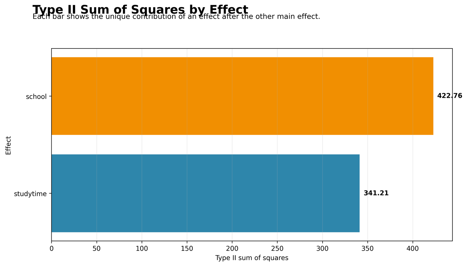
The first chart shows that school has the larger Type II SS at about 422.76. Studytime also explains a substantial unique portion, about 341.21.
Because these are Type II sums of squares, each bar represents a main effect after the other main effect has already been considered. This is the key difference from Type I SS, where the first term in the model receives credit first.
Python Chart 2: Mean G3 by Studytime
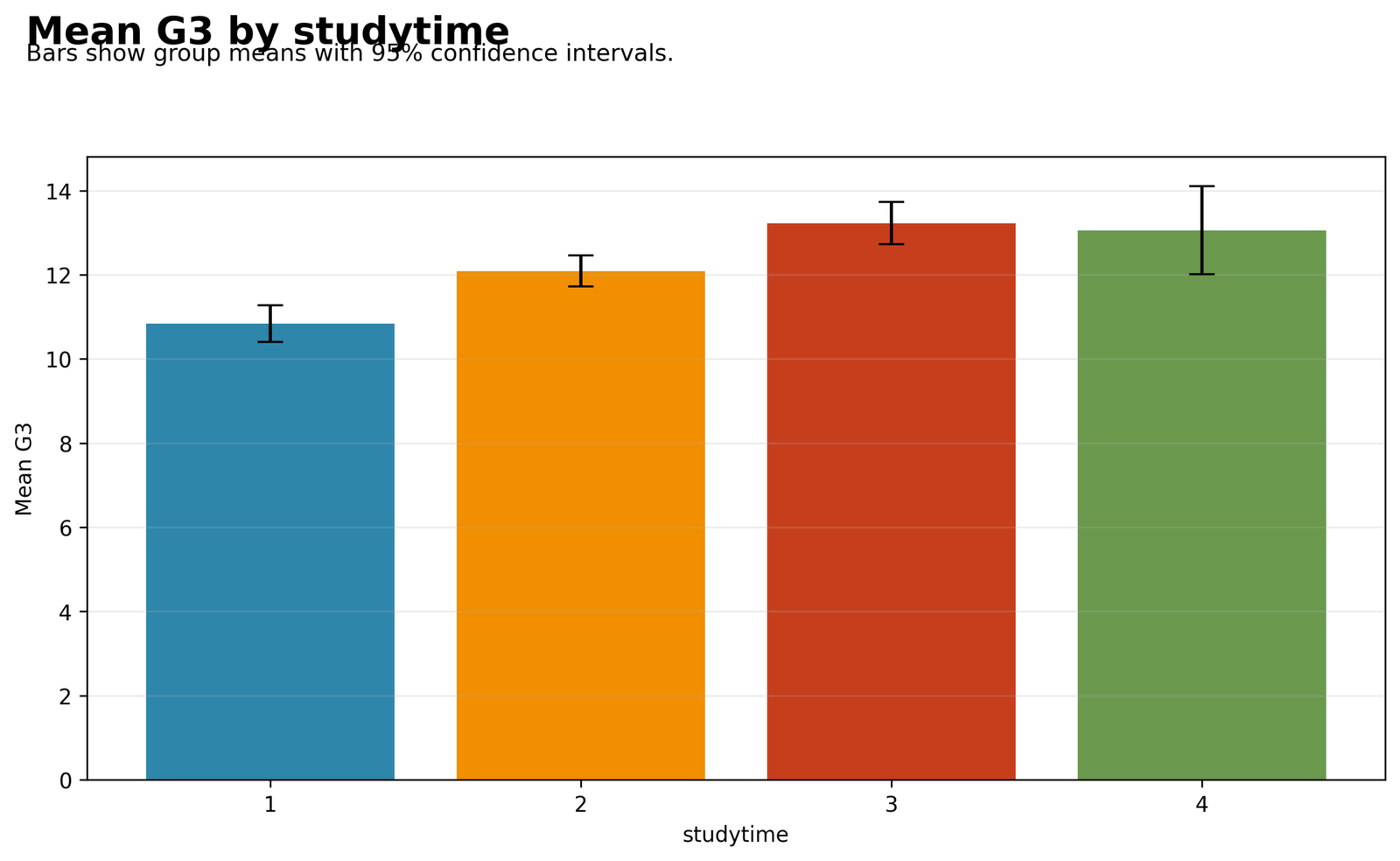
The studytime chart shows a clear upward pattern from studytime 1 to studytime 3, with studytime 4 remaining high. Studytime 1 has the lowest mean G3, while studytime 3 has the highest visible mean.
This mean pattern explains why studytime is significant in the Type II ANOVA table. The factor still explains unique G3 variation even after school is accounted for.
Python Chart 3: Mean G3 by School
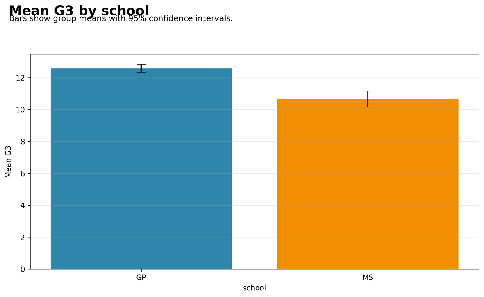
The school chart shows that GP has a higher mean G3 than MS. The visual gap between the bars is large and agrees with the significant school effect in the Type II table.
School has the larger Type II SS and larger partial eta squared in this example. This means school is the stronger of the two additive main effects.
Python Chart 4: Two-Factor Cell Mean Pattern
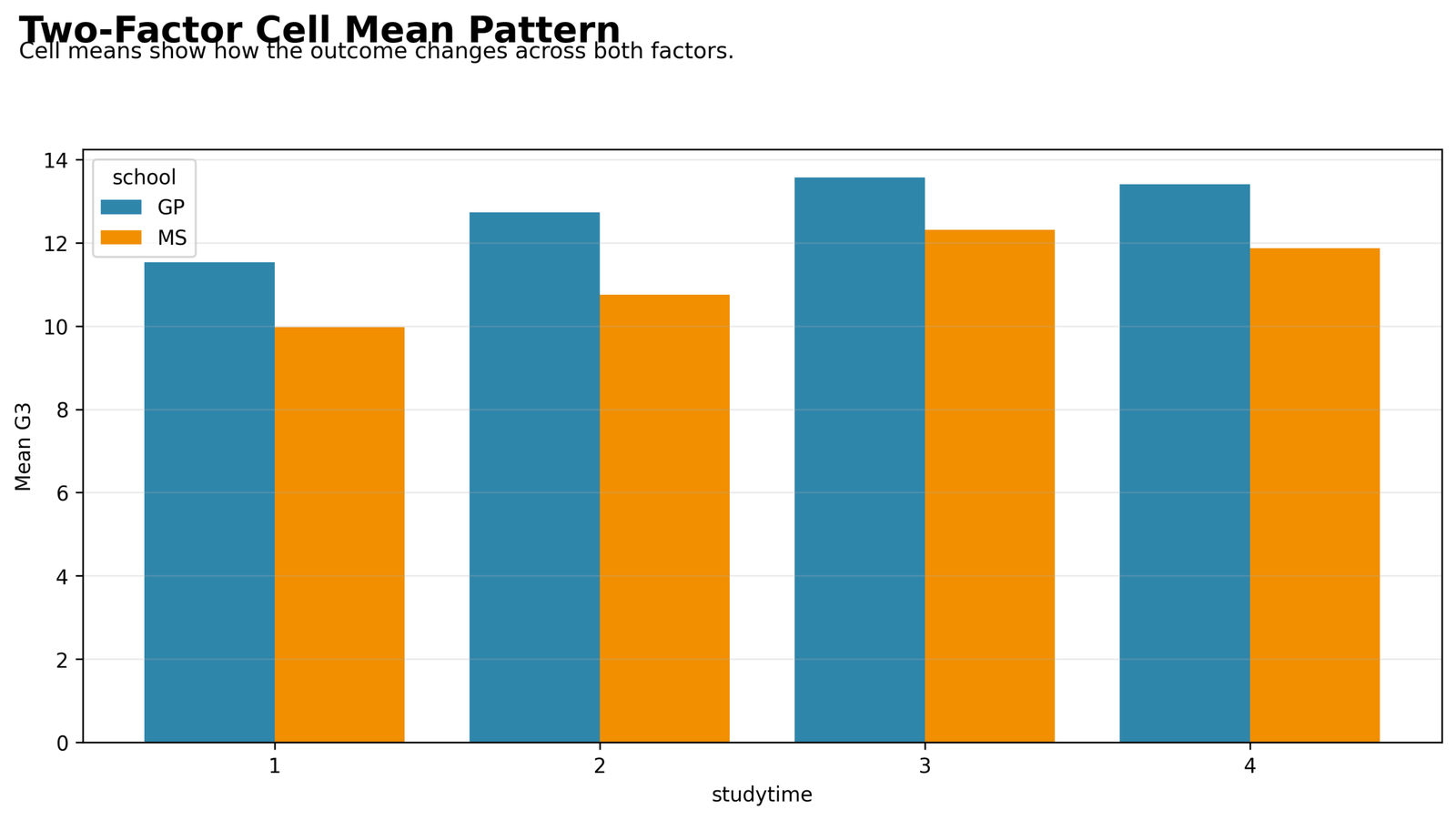
The cell mean chart shows that GP is higher than MS across all studytime groups. Both schools rise from studytime 1 toward studytime 3, while studytime 4 remains high but is based on smaller cells.
This chart is descriptive in the Type II additive workflow. It helps explain the main-effect pattern, but it is not itself a formal interaction test in this specific SPSS model.
Python Chart 5: Type II ANOVA F Statistics
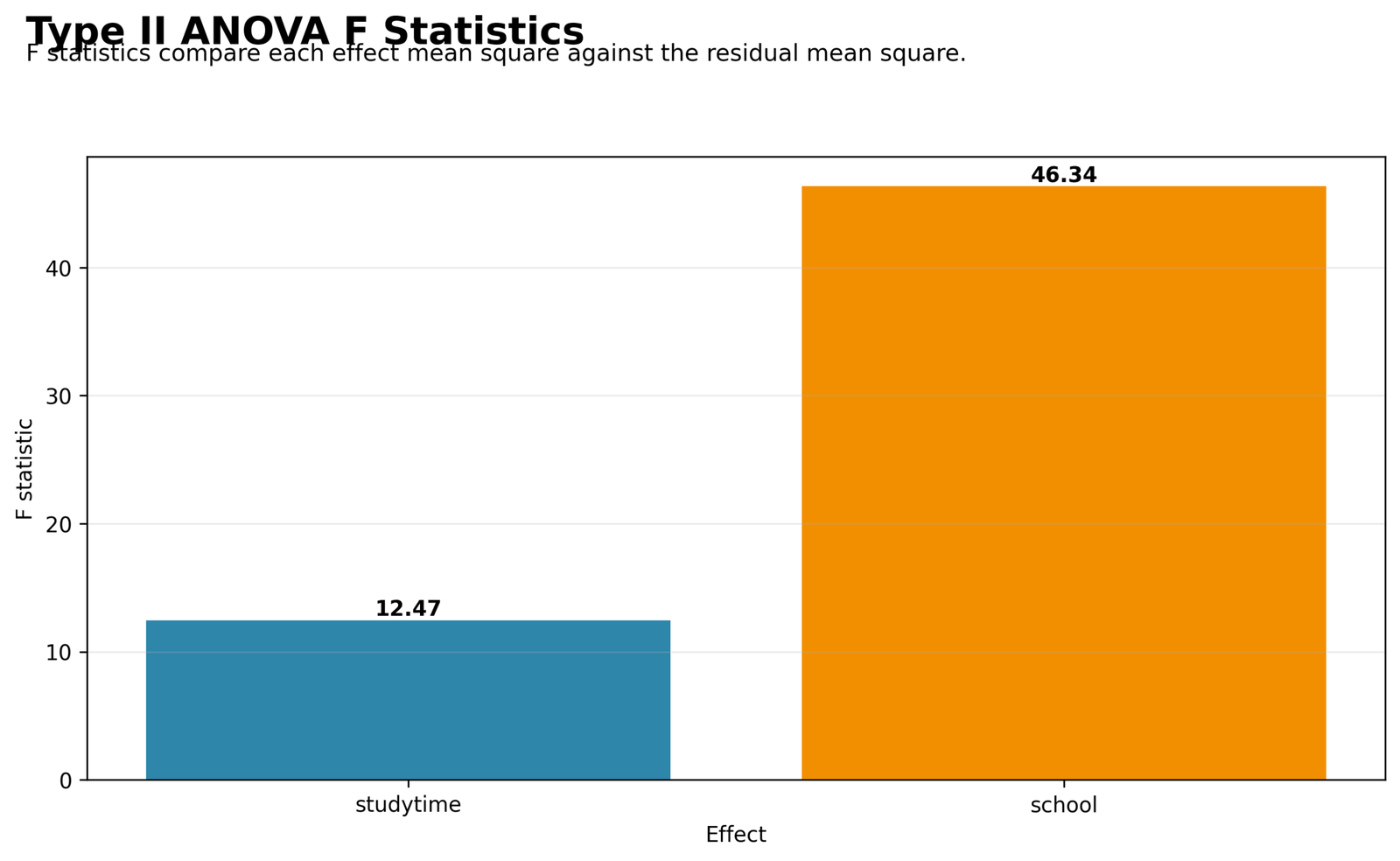
The F statistic chart shows that school has the stronger test statistic, about 46.34. Studytime has a smaller but still strong F statistic, about 12.47.
This chart supports the same decision as the summary table. Both main effects are statistically significant, with school providing the stronger adjusted main-effect signal.
Python Chart 6: Type II p-value Decision
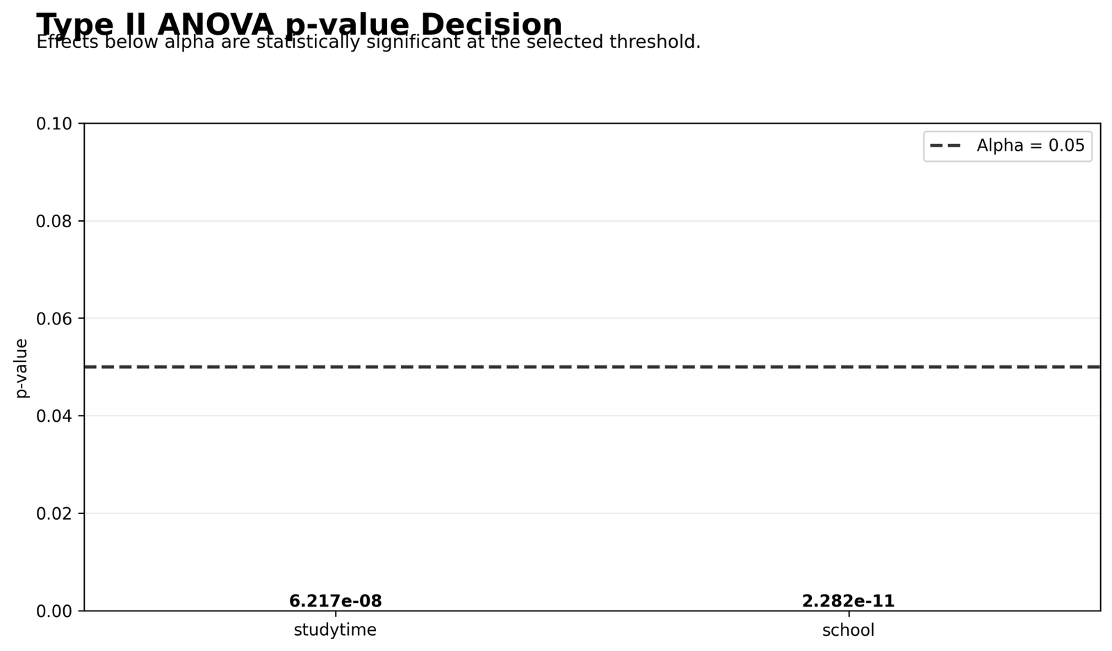
The p-value chart shows that both studytime and school are far below the alpha = .05 line. Studytime has p = 6.217e-08, and school has p = 2.282e-11.
This is the clearest decision chart. Both Type II main effects should be reported as statistically significant.
Python Chart 7: Residuals vs Fitted Values
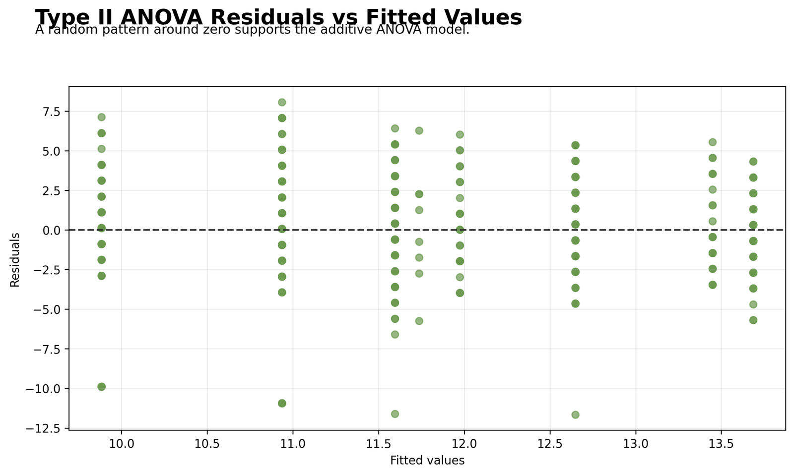
The residual plot shows vertical fitted-value bands because the model predicts group means from categorical factors. Most residuals sit around zero, but some large negative residuals are visible.
This means the additive model captures the group mean pattern, but individual students can still be far from their fitted group mean. The significant Levene result also means variance differences should be acknowledged.
Python Chart 8: Type II Summary Table
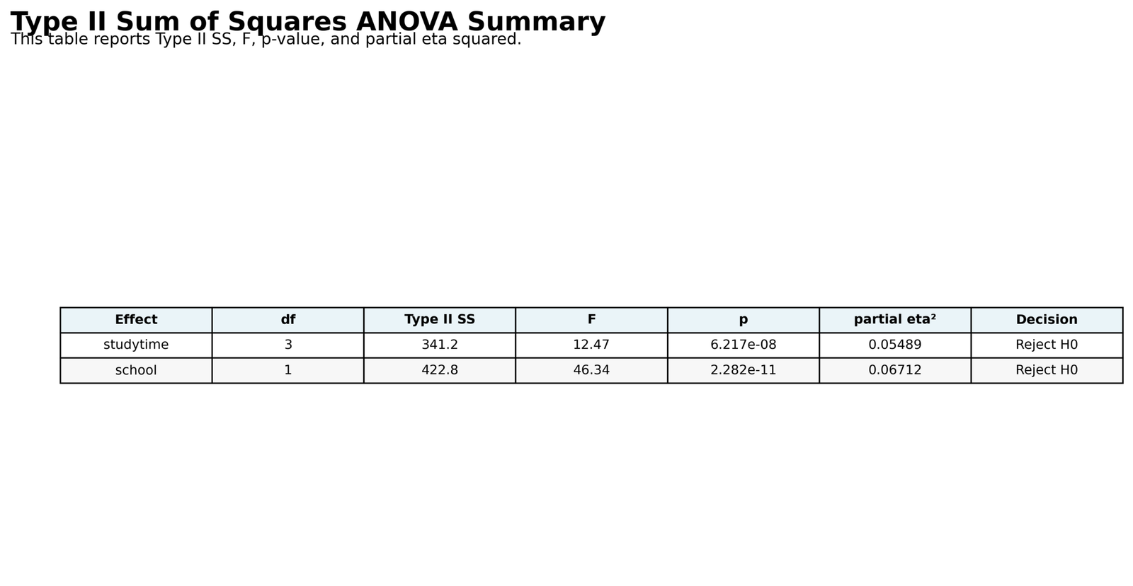
The summary table gives the final Python result in one place. Studytime and school are both significant, and both have small-to-moderate partial eta squared values.
This is the best table for reporting because it shows the formal Type II SS values, degrees of freedom, F statistics, p-values, effect sizes and decisions.
R Chart-by-Chart Validation
The R charts repeat the same Type II SS workflow in a second software environment. The R results confirm the Python and SPSS interpretation: studytime and school are both significant Type II main effects in the additive model.
R Chart 1: Type II Sum of Squares by Effect
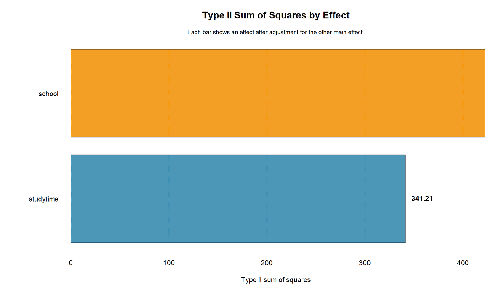
The R chart confirms that school has the larger Type II SS, while studytime still contributes a meaningful unique amount.
This software agreement supports the conclusion that the result is not caused by one package or plotting method.
R Chart 2: Mean G3 by Studytime
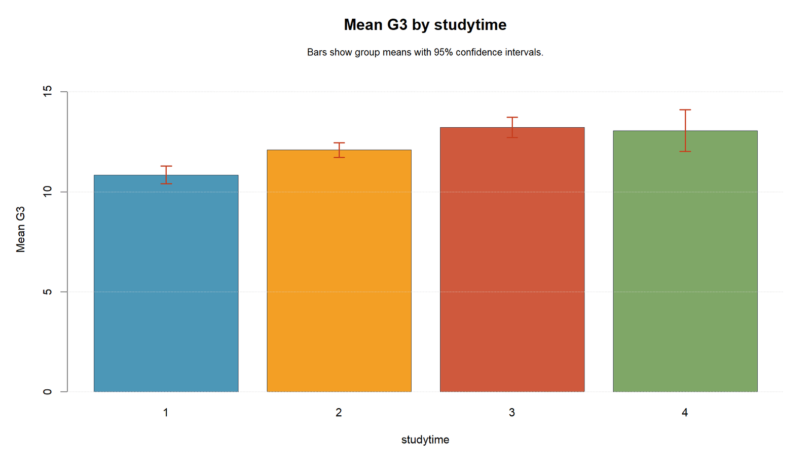
The R studytime chart confirms the same upward mean pattern from low studytime toward higher studytime levels.
This validates studytime as a significant main effect in the additive Type II ANOVA model.
R Chart 3: Mean G3 by School
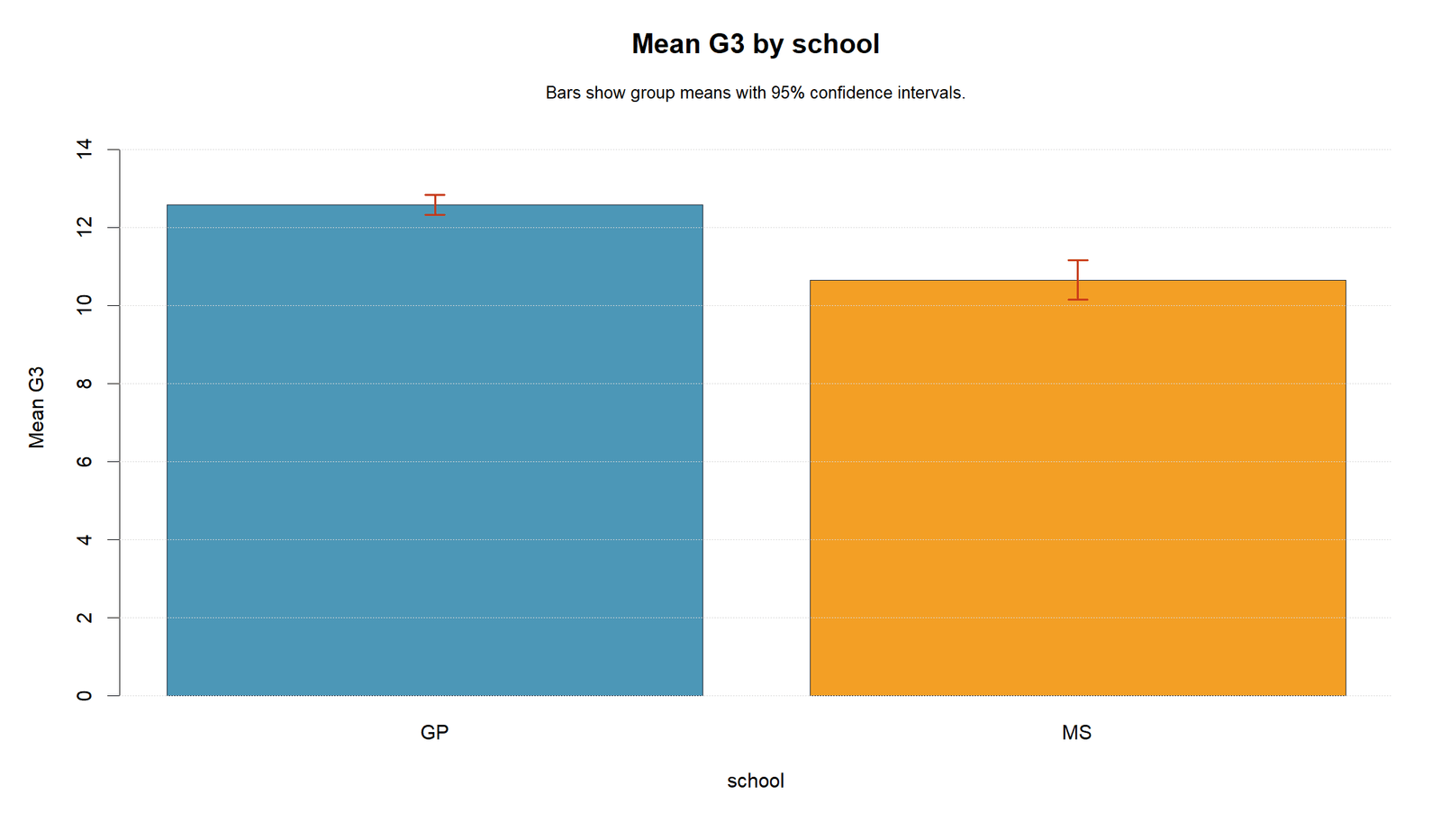
The R school chart confirms that GP has a higher mean G3 than MS.
This agrees with the larger school F statistic and larger school partial eta squared.
R Chart 4: Two-Factor Cell Mean Pattern
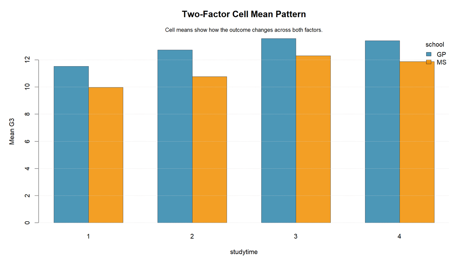
The R cell mean chart confirms the same descriptive pattern: GP is higher than MS across the studytime levels, and higher studytime groups generally have higher means.
This chart is useful for explaining the main effects but should not be described as the formal Type II interaction result because the Type II model here is additive.
R Chart 5: Type II ANOVA F Statistics
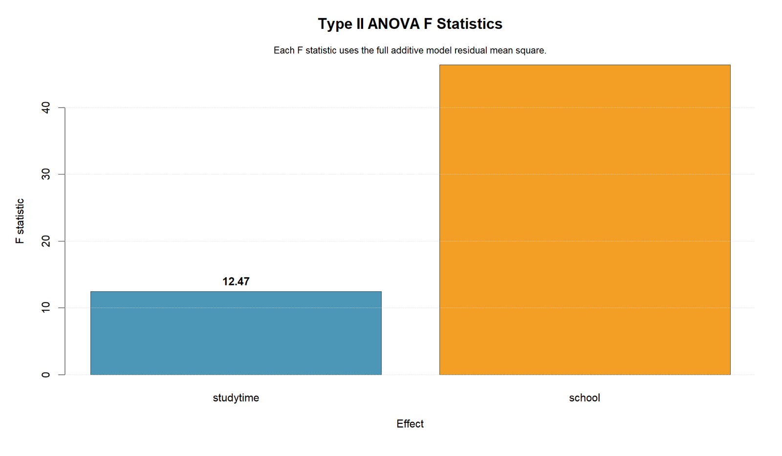
The R F statistic chart confirms that school has the strongest F statistic and studytime has a smaller but still statistically strong F statistic.
This supports the same effect-strength ranking as Python and SPSS.
R Chart 6: Type II p-value Decision
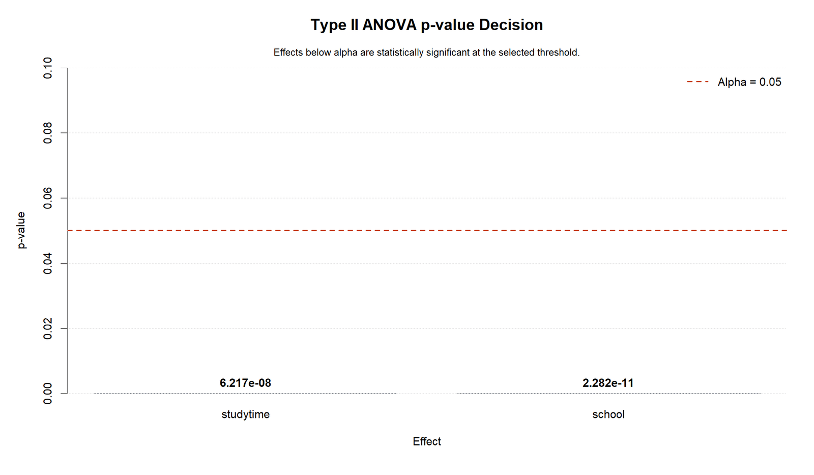
The R p-value chart confirms that both Type II effects are far below the .05 threshold.
This validates the final decision that studytime and school are significant unique main effects.
R Chart 7: Residuals vs Fitted Values
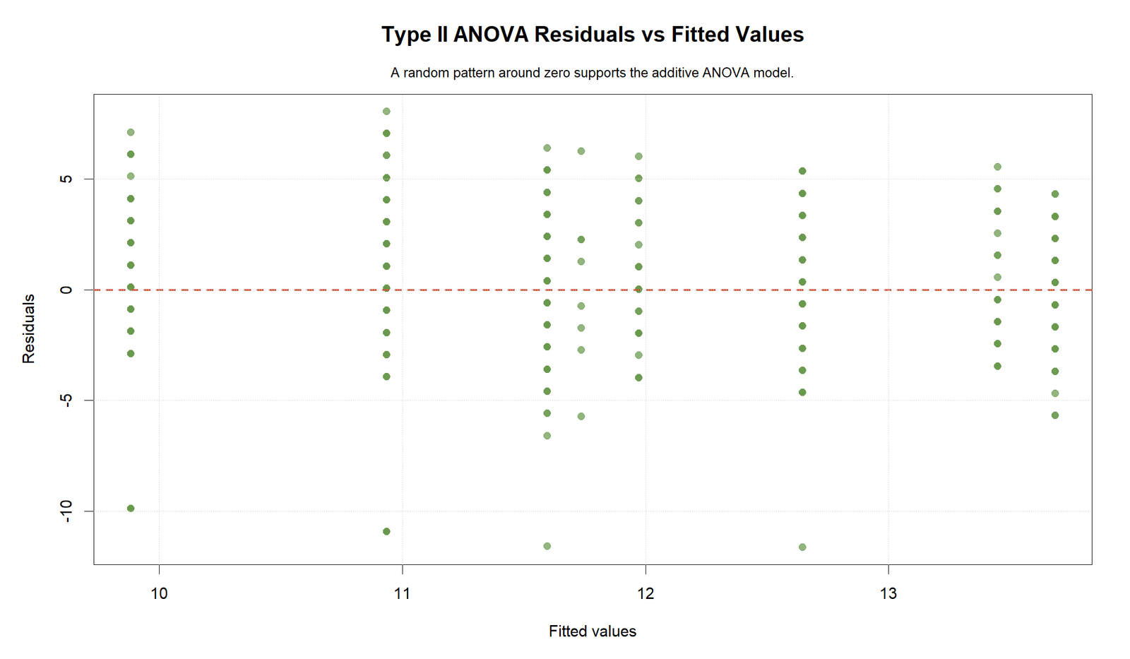
The R residual plot confirms the same diagnostic pattern as Python. Residuals are centered around zero, but some large negative residuals remain visible.
This supports a transparent assumption statement in the final report, especially because Levene’s test is significant.
R Chart 8: Type II Summary Table
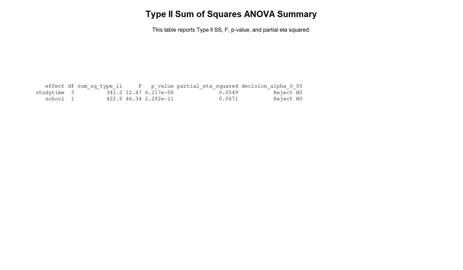
The R summary table confirms the same final result as Python and SPSS. Studytime and school are statistically significant in the additive Type II model.
This agreement across tools makes the interpretation stable for a teaching article and practical reporting.
SPSS, R, Python and Excel Workflows for Type II Sum of Squares
The same Type II Sum of Squares workflow can be reproduced in SPSS, R, Python and Excel. SPSS requires /METHOD=SSTYPE(2). R often uses the car::Anova() function for Type II SS. Python can use statsmodels.stats.anova.anova_lm(..., typ=2). Excel can support the concept through reduced-model comparisons, but SPSS, R or Python is better for final reporting.
SPSS Workflow
| Step | SPSS Menu or Syntax | Purpose |
|---|---|---|
| Open dataset | File > Open > Data | Load G3, studytime and school. |
| Use GLM Univariate | Analyze > General Linear Model > Univariate | Run the ANOVA model. |
| Set dependent variable | G3 | Define the numeric outcome. |
| Set fixed factors | studytime and school | Define the categorical factors. |
| Set Type II SS | /METHOD=SSTYPE(2) | Request Type II sums of squares. |
| Use additive design | /DESIGN=studytime school_id | Test the two main effects. |
| Read output | Tests of Between-Subjects Effects | Interpret Type II SS, F, p and partial eta squared. |
R Workflow
| Step | R Action | Purpose |
|---|---|---|
| Read data | read.csv("dataset.csv") | Load the dataset. |
| Convert factors | factor(studytime), factor(school) | Define categorical variables. |
| Fit additive model | lm(G3 ~ studytime + school) | Fit the Type II main-effects model. |
| Get Type II table | car::Anova(model, type = 2) | Report Type II SS. |
| Check cell means | group_by(studytime, school) | Explain the descriptive pattern. |
| Create diagnostics | Residual plot and assumption checks | Support final reporting. |
Python Workflow
| Step | Python Action | Purpose |
|---|---|---|
| Read data | pandas.read_csv() | Load G3, studytime and school. |
| Fit model | ols("G3 ~ C(studytime) + C(school)") | Fit the additive ANOVA model. |
| ANOVA table | anova_lm(model, typ=2) | Get Type II sums of squares. |
| Effect sizes | Calculate partial eta squared | Report practical size. |
| Means | Group means and confidence intervals | Explain studytime and school patterns. |
| Diagnostics | Residuals vs fitted | Check model assumptions. |
Excel Workflow
| Excel Task | Formula or Tool | Purpose |
|---|---|---|
| Prepare data | Columns for G3, studytime and school | Organize the ANOVA dataset. |
| Create PivotTable | Rows = studytime, Columns = school, Values = Average G3 | Summarize cell means. |
| Create dummy variables | Studytime and school dummies | Build reduced and full models. |
| Reduced model for studytime | Model with school only | Compare to full additive model. |
| Reduced model for school | Model with studytime only | Compare to full additive model. |
| Formal Type II table | Use SPSS, R or Python | Best option for publishable output. |
Code Blocks for Type II Sum of Squares
SPSS Syntax for Type II Sum of Squares
* Type II Sum of Squares in SPSS.
* Dependent variable: G3.
* Additive model: studytime + school_id.

TITLE "Type II Sum of Squares: G3 by Studytime and School".

UNIANOVA G3 BY studytime school_id
  /METHOD=SSTYPE(2)
  /INTERCEPT=INCLUDE
  /PRINT=DESCRIPTIVE ETASQ HOMOGENEITY PARAMETER
  /CRITERIA=ALPHA(.05)
  /DESIGN=studytime school_id.

OUTPUT EXPORT
  /CONTENTS EXPORT=VISIBLE
  /PDF DOCUMENTFILE="type_ii_sum_of_squares_spss_output.pdf".
Python Code for Type II Sum of Squares
import pandas as pd
from statsmodels.formula.api import ols
from statsmodels.stats.anova import anova_lm

df = pd.read_csv("dataset.csv")

df["G3"] = pd.to_numeric(df["G3"], errors="coerce")
df["studytime"] = df["studytime"].astype("category")
df["school"] = df["school"].astype("category")

data = df[["G3", "studytime", "school"]].dropna().copy()

# Additive model for Type II Sum of Squares
model = ols("G3 ~ C(studytime) + C(school)", data=data).fit()

type2_table = anova_lm(model, typ=2)

error_ss = type2_table.loc["Residual", "sum_sq"]
type2_table["partial_eta_sq"] = type2_table["sum_sq"] / (
    type2_table["sum_sq"] + error_ss
)

print(type2_table)

# Group means
print(data.groupby("studytime")["G3"].agg(["count", "mean", "std"]))
print(data.groupby("school")["G3"].agg(["count", "mean", "std"]))
print(data.groupby(["studytime", "school"])["G3"].agg(["count", "mean", "std"]))

# Residual diagnostics
data["fitted"] = model.fittedvalues
data["residual"] = model.resid
print(data[["G3", "studytime", "school", "fitted", "residual"]].head())
R Code for Type II Sum of Squares
# Type II Sum of Squares in R

library(tidyverse)

df <- read.csv("dataset.csv")

df$G3 <- as.numeric(df$G3)
df$studytime <- as.factor(df$studytime)
df$school <- as.factor(df$school)

data <- df %>%
  select(G3, studytime, school) %>%
  drop_na()

# Additive model
model_type2 <- lm(G3 ~ studytime + school, data = data)

# Type II sums of squares
# install.packages("car")
library(car)
Anova(model_type2, type = 2)

# Cell means
data %>%
  group_by(studytime, school) %>%
  summarise(
    n = n(),
    mean_G3 = mean(G3),
    sd_G3 = sd(G3),
    .groups = "drop"
  )

# Diagnostics
par(mfrow = c(1, 2))
plot(fitted(model_type2), residuals(model_type2),
     xlab = "Fitted values", ylab = "Residuals",
     main = "Residuals vs Fitted")
abline(h = 0, lty = 2)
qqnorm(residuals(model_type2))
qqline(residuals(model_type2))
Excel Notes for Type II Sum of Squares
Excel support workflow:

1. Arrange the data:
   G3 | studytime | school

2. Create a PivotTable:
   Rows = studytime
   Columns = school
   Values = average of G3, count of G3, standard deviation of G3

3. Create reduced and full additive models:
   Reduced model for studytime: G3 = school
   Reduced model for school: G3 = studytime
   Full additive model: G3 = studytime + school

4. Calculate Type II SS:
   SS_studytime = SSE_school_only - SSE_full_additive
   SS_school = SSE_studytime_only - SSE_full_additive

5. Calculate F statistics:
   F = MS_effect / MS_error

6. Formal Type II ANOVA:
   Use SPSS, R or Python for the final publishable table.
APA Reporting Wording
When reporting Type II Sum of Squares, mention that the model was additive and that each main effect was tested after the other main effect. Also report effect sizes and assumption context.
APA-style report: A two-factor additive ANOVA using Type II Sum of Squares was conducted to examine G3 final grade by studytime and school. The additive model was significant, F(4, 644) = 24.329, p < .001, R² = .131, adjusted R² = .126. Studytime explained significant unique variation in G3 after school was accounted for, F(3, 644) = 12.467, p < .001, partial η² = .055. School also explained significant unique variation in G3 after studytime was accounted for, F(1, 644) = 46.339, p < .001, partial η² = .067. Levene’s test was significant, F(7, 641) = 3.384, p = .001, so the homogeneity of variance assumption should be interpreted cautiously.
Short reporting version: Using Type II Sum of Squares in an additive model, both studytime and school were significant predictors of G3. School had the larger unique effect, but studytime also explained significant G3 variation after school was controlled.
Common Mistakes
| Mistake | Why It Is Wrong | Correct Practice |
|---|---|---|
| Confusing Type II SS with Type I SS | Type I is sequential; Type II tests main effects after other main effects. | State the SS type clearly. |
| Using Type II SS when interaction is central | Type II main effects are not tested after the interaction. | Use a full factorial model and consider Type III SS when interaction is important. |
| Calling the cell mean chart an interaction test | The SPSS Type II model here is additive and does not include an interaction term. | Use the cell chart descriptively only. |
| Ignoring Levene’s test | The output shows variance assumption pressure. | Report assumption caution and compare robust methods if needed. |
| Reporting only p-values | P-values do not show practical importance. | Report partial eta squared with each effect. |
| Using Excel as the only formal tool | Excel is not ideal for Type II ANOVA tables. | Use SPSS, R or Python for the final Type II SS output. |
When to Use Type II Sum of Squares
Use Type II Sum of Squares when the main-effects model is the primary research question and interaction is not central. Type II SS is often preferred over Type I SS when the researcher does not want results to depend on model-entry order.
| Situation | Use Type II SS? | Reporting Note |
|---|---|---|
| Additive two-factor ANOVA | Yes | Type II SS is suitable for unique main effects. |
| Balanced design with no interaction focus | Often yes | Type I, II and III may be closer when design is balanced. |
| Unbalanced design with main-effect focus | Often useful | Type II avoids Type I order dependence. |
| Important interaction term | Use caution | Consider Type III SS and interaction interpretation. |
| Planned hierarchical model | Not usually | Type I SS may be better if order is theoretically planned. |
Compare this guide with Factorial ANOVA, One Way ANOVA, Two Way ANOVA, Balanced ANOVA, Fixed Effects ANOVA, Brown Forsythe ANOVA, ANOVA Effect Size, ANOVA in SPSS, ANOVA in R and ANOVA in Python.
Downloads and Resources for Type II Sum of Squares
Use these resources to reproduce the Type II Sum of Squares workflow. The Python report, R report and SPSS output PDF are included as verification files. Script and workbook placeholders can be replaced after the final downloadable files are uploaded to the WordPress Media Library.
Download Dataset
Practice dataset with G3, studytime and school variables.
Download Type II Sum of Squares Python Report PDF
Python report PDF for Type II SS, F statistics, p-values, means and diagnostics.
Download Type II Sum of Squares R Report PDF
R validation PDF for additive Type II ANOVA interpretation.
Download Type II Sum of Squares SPSS Output PDF
SPSS output PDF using SSTYPE(2) for Type II sums of squares.
Download Python Script
Python code for Type II ANOVA tables, effect sizes and charts.
Download R Script and Excel Workbook
R workflow and Excel support workbook for Type II sums of squares.
FAQs About Type II Sum of Squares
What is Type II Sum of Squares?
Type II Sum of Squares tests each main effect after the other main effects in an additive ANOVA model, but not after interaction terms.
What was tested in this example?
The example tested G3 final grade by studytime and school using an additive Type II ANOVA model.
Was studytime significant?
Yes. Studytime was statistically significant, with p = 6.217e-08 in the Python summary and p < .001 in SPSS.
Was school significant?
Yes. School was statistically significant, with p = 2.282e-11 in the Python summary and p < .001 in SPSS.
Which effect was larger?
School was larger in this output, with Type II SS about 422.8 and partial eta squared about 0.067.
How is Type II Sum of Squares different from Type I Sum of Squares?
Type I SS is sequential and depends on model order. Type II SS tests each main effect after the other main effects, so it is not interpreted as a model-entry sequence.
How is Type II Sum of Squares different from Type III Sum of Squares?
Type III SS tests each effect after all other effects, including interactions. Type II SS focuses on main effects after other main effects and is best for additive models.
Does SPSS report Type II Sum of Squares by default?
No. In SPSS syntax, Type II SS should be requested with /METHOD=SSTYPE(2).
Can Type II Sum of Squares be done in Excel?
Excel can approximate Type II SS using reduced-model comparisons, but SPSS, R or Python is better for a formal publishable Type II ANOVA table.
How do I report this Type II Sum of Squares result?
A concise report is: Using Type II Sum of Squares in an additive ANOVA model, both studytime and school explained significant unique variation in G3.

