
Savage Scores Test: 7 Essential Steps, Formula and Worked Example
The Savage Scores Test is a nonparametric two-sample linear-rank procedure that gives progressively greater weight to the largest pooled observations. This complete guide explains the assumptions, exponential-order-statistic scores, tie handling, worked school-absence example, interpretation, and reproducible workflows in Python, R, SPSS, Excel, MATLAB and SAS.
The upper tail of student absences was significantly heavier in the GP school group.
In this worked Savage Scores Test example, absence counts from 423 GP students and 226 MS students were pooled, ordered and converted to tie-adjusted Savage scores. The GP score sum was S = 472.944205, compared with E(S) = 423 under random group labels. The standardized result was z = 4.162644 with p = 0.00003146. At α = .05, the equal-distribution null was rejected.
What does the Savage Scores Test measure?
An upper-tail-sensitive answer to a two-sample distribution question.
The Savage Scores Test is a two-sample linear-rank procedure whose exponential-order-statistic scores rise sharply near the largest pooled values. It is designed for scientific questions in which unusually high observations matter more than ordinary differences near the center.
The target of inference
The test asks whether the two independent groups are exchangeable once the largest pooled values receive special emphasis. This is not the same as asking whether group means differ, whether medians differ, or whether variances are equal. A test result becomes significant when one group accumulates more upper-tail-sensitive rank scores than expected under the null hypothesis of identical distributions under random labeling.
Because the test is rank-based, it remains useful when the observed outcome is skewed, zero-inflated, discrete, heavy-tailed or punctuated by a few very large values. In such settings, a classical t test may overemphasize modeling assumptions that are not central to the research problem. The Savage Scores Test uses the order structure of the data and then translates the largest ranks into progressively larger harmonic scores.
Why the upper tail matters
Suppose two clinics have similar typical waiting times but one clinic has many more extreme delays, or two schools have similar median absences but one has more students with very large absence counts. A general rank test such as the Mann–Whitney U test may still detect a difference, but the test deliberately gives more importance to the extreme observations that define the scientific concern. That is why the test can be more informative when the key issue is not the center of the distribution, but the severity of the worst outcomes.
In the present worked example, the outcome is student absences and the two groups are schools. The Savage Scores Test is well suited because the absence distribution contains many low values but also some much larger observations. Those large counts matter practically: they represent students whose absence burden is substantively more serious than the typical case.
When should you use the Savage Scores Test?
Use the decision logic before opening software.
Use the Savage Scores Test for exactly two independent groups when the outcome is orderable and the prespecified concern is a heavier upper tail. Do not choose it merely because a normality check was significant.
The test is not a generic default for every two-sample problem. It is the right choice when you can defend all of the following: there are exactly two independent groups; the outcome can be ordered from smallest to largest; you expect the most informative difference to occur near the upper tail; and a rank-based procedure is preferable to a fully parametric model. When those conditions hold, the test can be both interpretable and powerful.
Two groups
The Savage Scores Test is a two-sample method. If you have three or more independent groups, think first about a broader method such as the Kruskal–Wallis test or another omnibus procedure.
Independent observations
Each measurement should belong to one group only. Paired, blocked or repeated-measures designs need different methods, such as the Friedman test, Quade test or Page’s trend test.
Ordered outcome
The test needs values that can be pooled and ranked. Counts, times, scores, biomarker levels and ordered numeric responses are typical candidates.
Upper-tail concern
The reason to prefer the test is its explicit upper-tail weighting. If your question is about the center, use the Mann–Whitney U test instead.
Tie-aware reporting
Many practical datasets contain ties. The test remains usable, but tied positions must receive averaged scores and the tie rule must be reported clearly.
The Savage Scores Test is especially attractive in policy, education, clinical, industrial and service settings where the worst values are the values that trigger action. A school administrator may care less about whether two schools differ by a fraction of an absence on average and more about whether one school produces far more students with very high absence burdens. A quality engineer may care more about the most extreme cycle times than about median shifts. A hospital may care more about the tail of waiting time than about ordinary cases. In those situations, the test matches the language of the decision problem.
By contrast, if the tail is not the main focus, the test may be an awkward choice. For location differences, consider the Mann–Whitney U test or Brunner–Munzel test. For scale, consider the Ansari–Bradley test or Moses test of extreme reactions. For a broad shape-sensitive comparison, the two-sample Kolmogorov–Smirnov test may be more appropriate.
Savage Scores Test assumptions: six conditions to check
The method is nonparametric, but it is not assumption-free.
The main Savage Scores Test assumptions concern independence, meaningful ordering, random-label exchangeability, an upper-tail-focused research question, transparent tie handling and a suitable exact, asymptotic or permutation reference distribution.
Core assumptions
What the test does not assume
The Savage Scores Test does not require normality, equal variances or interval-scale measurement in the same way that a t test would. That is one reason many analysts move toward the test after reviewing the outcome distribution, histograms and outliers. You can revisit supporting topics through descriptive statistics, histogram interpretation and outlier detection.
Still, nonparametric does not mean “free from design thinking.” If the groups are not independent, if the tail emphasis is unjustified, or if the observations are the result of severe measurement heaping that destroys meaningful ordering, the test can be a poor match even though it is technically easy to compute.
The most common misunderstanding is to treat the test as a mysterious black box that simply replaces a t test. That is too vague. The Savage Scores Test works because the scoring system reflects a specific alternative: more mass in the upper tail for one group. Analysts should say this explicitly. When the research objective is aligned with that emphasis, the test becomes easier to defend and easier for readers to understand.
Savage Scores Test hypotheses: upper-tail score concentration
State the focus group and direction before interpreting the sign.
The null hypothesis for the Savage Scores Test states that group labels are exchangeable with respect to the pooled Savage score vector. The alternative states that one group accumulates more or less upper-tail score mass than expected.
Null hypothesis
H0: the two groups come from the same underlying distribution under exchangeable labels. Under the null, neither group should accumulate an unusually large share of the upper-tail-sensitive Savage scores.
Alternative hypothesis
HA: one group tends to have larger upper-tail-sensitive scores than expected, meaning the distributions differ in a direction that is most visible among the largest values.
Used when either group could have the heavier upper tail.
Used when theory states in advance which group is expected to contribute more extreme high values.
A positive z means the focus group has a larger score sum than expected. A negative z means it has a smaller score sum than expected.
In the worked example, the focus group is GP. The test statistic sums the Savage scores observed in GP. Because the result is positive, the GP group receives more upper-tail weight than expected under the null hypothesis. If the research question had defined MS as the focus group instead, the same result would appear with the sign reversed and the same two-sided p-value.
Explicitly stating the focus group prevents confusion. Readers should know whether the reported score sum belongs to GP, MS, the first listed category or the category of theoretical interest. This matters because the test is usually communicated through one group’s score total rather than through a symmetric difference statistic like a mean difference.
Savage Scores Test formula, scores and large-sample calculation
The score system is based on expected exponential order statistics.
The Savage Scores Test formula assigns a harmonic score to each pooled position, averages the occupied position scores within tied blocks, sums the resulting scores in one group and standardizes that sum using the random-label expectation and variance.
For the Savage Scores Test, i is the pooled rank position from smallest to largest and N is the total sample size. The largest position receives the largest Savage score.
The test statistic S is the sum of the Savage scores belonging to the chosen focus group. Here, the focus group is GP.
The expectation and finite-population permutation variance are computed from the full set of pooled scores. In this data, the average Savage score is 1, so the expected score sum equals n1 = 423.
The large-sample This test compares the standardized statistic to the standard normal distribution. The two-sided p-value is 2P(|Z| ≥ |zobs|).
The brilliance of the test is that the score increments are not linear. As the pooled positions move closer to the largest observed values, the harmonic score continues to increase. That means an observation near the very top of the ordered sample influences the Savage Scores Test more strongly than an observation in the middle. The test is therefore a purposeful compromise between a pure tail method and a full-distribution rank method.
Ties deserve special treatment. In a dataset with tied outcome values, several observations occupy a block of pooled positions. The correct tie-aware This test assigns each tied observation the average of the Savage scores associated with those occupied positions. That is exactly how the uploaded workbook was built. Without this averaging step, the test statistic depends on arbitrary ordering within ties, which would be indefensible.
Why the expected score sum equals 423
The full pooled set of Savage scores has mean 1. Therefore the expected total in any group of size n1 under random labels is simply n1. This property makes the test surprisingly transparent: once you know the observed score sum, you can immediately see whether the group has accumulated more or less upper-tail weight than expected.
Savage Scores Test example: student absence distributions
A complete two-school comparison using all 649 student records.
This Savage Scores Test example compares absence distributions for GP and MS students. It documents the outcome and grouping variables, group sizes, descriptive summaries, score construction, tie rule and every numerical component of the final statistic.
| Role | Variable | Description | Observed values in this guide |
|---|---|---|---|
| Outcome | absences | Student absence count, ordered from low to high before score assignment. | 0 to 32 |
| Grouping variable | school | Independent two-level factor indicating school group. | GP and MS |
| Focus group | GP | Group whose Savage score sum is reported as the main statistic. | n = 423 |
| Comparison group | MS | Second independent group. | n = 226 |
| Score variable | Savage score | Tie-adjusted harmonic upper-tail score assigned to each pooled observation. | 0.218081 to 7.053419 |
The raw outcome is discrete and heavily tied, with many students at 0, 1, 2, 4 or 6 absences. That is exactly the sort of data structure where the test remains useful: it does not demand normality or equal variances, yet it still respects the ordered nature of the outcome. The value range is wide, extending from no absences up to 32 in the GP group. This wide range is important because it creates the extreme upper values that the Savage Scores Test is designed to emphasize.
The descriptive summaries already hint at the final result. Both groups share the same median absences value of 2, but the upper quartile is higher in GP (6) than in MS (4), and the maximum is much larger in GP (32) than in MS (12). Those summaries do not replace the test, but they help explain why the test flags a significant upper-tail difference even when a simple center-based description might look less dramatic.
Step 1: order the pooled absences
The Savage Scores Test begins by pooling all 649 absences values across the two schools and sorting them from smallest to largest. Unlike a t test, the test does not use raw deviations from a mean. Instead, it translates the order information into position-specific scores. In this dataset, many low values repeat, so ties occupy blocks of positions.
Because ties are frequent, the test averages the occupied position scores within each tie block. For example, all students with the same absence count receive the same average Savage score. That is why the score variable is discrete even though it comes from an underlying position sequence.
Step 2: assign the upper-tail-sensitive scores
Observations near the bottom of the pooled distribution receive small Savage scores, while observations near the top receive larger scores. The score quartiles in the workbook are 0.218081, 0.657605 and, depending on group composition, around 1.493874. The highest score, 7.053419, belongs to the most extreme absence value in the pooled sample.
This is the defining feature of the test: it cares much more about the rare 24-, 26-, 30- and 32-absence students than about the difference between 0 and 1 absence. When extreme outcomes are what matter, that emphasis is a strength rather than a weakness.
Step 3: sum scores in the focus group
After score assignment, the workbook sums the Savage scores for the GP group. The observed Savage Scores Test score sum is 472.944205. Under random labeling, the expected total is 423. Therefore the GP group exceeds its null expectation by 49.944205 points, or roughly 11.81%.
That difference is not an arbitrary scale artifact. Because the scores heavily reward large pooled ranks, the excess score sum indicates that GP contains more high-end absence observations than would be expected if the schools had the same underlying distribution.
Step 4: standardize and test
The finite-population variance term is 143.956657, producing a standard deviation of 11.998194. The resulting standardized This test statistic is z = 4.162644. The two-sided p-value is 0.00003146, which is far below α = .05.
Therefore, the worked This test rejects the null hypothesis of equal distributions under exchangeable labels. The direction of the statistic shows that the upper tail is heavier in the GP group than in the MS group.
Worked example conclusion
The verified This test shows that the GP school group contributes significantly more upper-tail-sensitive absence scores than expected under the null. In plain language, the most extreme absence counts are more concentrated in GP than in MS.
z = 4.163, p = 3.1458e-05
Savage Scores Test statistics, results and interpretation
The verified result connects the score sum to the upper-tail conclusion.
The Savage Scores Test statistics show that the GP score sum is more than four standard errors above its random-label expectation. The two-sided result is highly significant and points to a heavier upper absence tail in GP.
Primary inference
Reject H0
The GP group accumulated substantially more upper-tail-sensitive score mass than expected under random labeling. The positive statistic points toward a heavier upper absence tail in GP.
Calculation audit
| Evidence component | Verified value | Interpretive role |
|---|---|---|
| Total sample | N = 649 | All observations were retained and scored. |
| Group composition | GP = 423; MS = 226 | Defines the random-label expectation and variance. |
| Observed minus expected | 49.944205 | GP accumulated more score mass than expected. |
| Two-sided significance | p = 0.00003146 | Strong evidence against exchangeable group labels. |
| Descriptive standardized index | |z|/√N = 0.163 | Small-to-moderate standardized magnitude; label it as descriptive. |
Savage Scores Test in Python: complete calculation and charts
A transparent NumPy, pandas and SciPy workflow.
The Savage Scores Test in Python is implemented by constructing the pooled exponential-order-statistic scores directly. The supplied charts then audit the group summaries, scored observations, score quantiles and final result.
Python is often the easiest place to explain a Savage Scores Test because the full pipeline can be written in readable steps: sort the pooled data, build the position scores, average within ties, sum scores inside the focus group, compute the expectation and variance, and standardize the result. None of these steps are obscure, but placing them in code removes ambiguity.
import numpy as np
import pandas as pd
from scipy.stats import norm# df contains two columns: absences and school.
df = pd.read_csv("student_absences.csv")
group_col = "school"
value_col = "absences"
focus_group = "GP"
# 1) Order the pooled values.
df = df.sort_values(value_col, kind="mergesort").reset_index(drop=True)
N = len(df)
# 2) Build Savage scores for positions 1..N.
# a_i = sum_{j=N-i+1}^N 1/j
harmonic_tail = np.array([
np.sum(1 / np.arange(N - i + 1, N + 1))
for i in range(1, N + 1)
])
# 3) Average positions inside ties.
df["rank"] = df[value_col].rank(method="average")
# Convert average rank to average Savage score by tie block.
score_lookup = {}
for value, sub in df.groupby(value_col, sort=True):
idx = sub.index.to_numpy()
score_lookup[value] = harmonic_tail[idx].mean()
df["savage_score"] = df[value_col].map(score_lookup)
# 4) Sum scores in one group.
S = df.loc[df[group_col] == focus_group, "savage_score"].sum()
n1 = (df[group_col] == focus_group).sum()
n2 = N - n1
# 5) Permutation expectation and variance.
a = df["savage_score"].to_numpy()
a_bar = a.mean()
var_pop = np.sum((a - a_bar) ** 2)
E = n1 * a_bar
V = (n1 * n2 / (N * (N - 1))) * var_pop
z = (S - E) / np.sqrt(V)
p_value = 2 * norm.sf(abs(z))
print({
"N": int(N),
"n1": int(n1),
"n2": int(n2),
"score_sum": float(S),
"expected": float(E),
"variance": float(V),
"z": float(z),
"p_value": float(p_value)
})
There are two practical points worth emphasizing. First, the test is defined on the pooled sample. You should not assign Savage scores inside each group separately. Second, ties must be scored by averaging over the occupied pooled positions. If the dataset is sorted but ties are resolved in an arbitrary observation order, the test is mis-implemented. The uploaded workbook and the code outline above both follow the correct tie-aware rule.
After execution, the Python workflow should return the same verified output shown in the article: 472.944205 for the GP score sum, 423 for the expectation, 143.956657 for the variance, 4.162644 for the z statistic and 0.00003146 for the two-sided p-value. If your numbers differ materially, the first places to debug are the tie handling and the group chosen for the score sum.
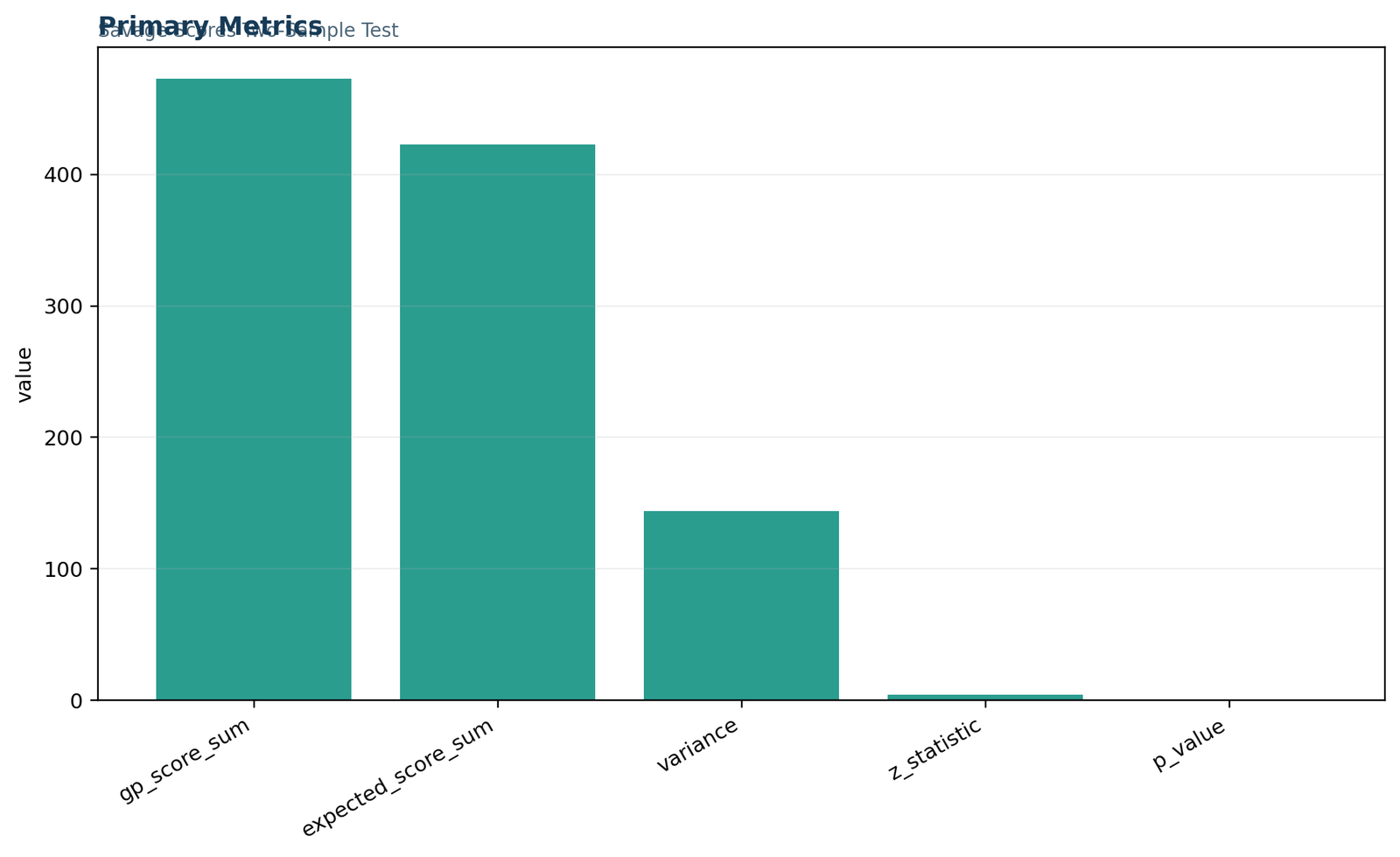
Python chart 1: primary metrics
This primary-metrics panel summarizes the verified This test values: N = 649, nGP = 423, nMS = 226, observed score sum = 472.944205, expectation = 423, z = 4.162644, and p = 0.00003146. It provides the compact statistical headline for readers who need the result quickly.
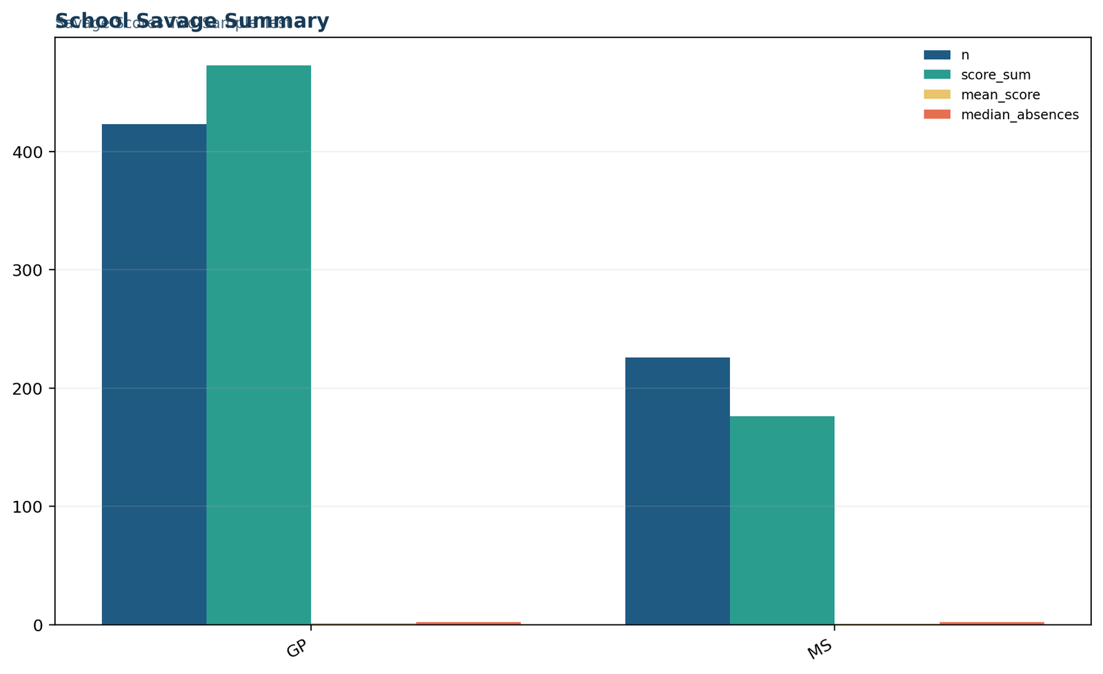
Python chart 2: school Savage score summary
This chart compares the group-wise Savage Scores Test score summaries. The GP group has a mean Savage score of 1.118 compared with 0.779 in MS. Because larger scores concentrate at the upper tail, the higher group mean is consistent with more severe high-end absences in GP.
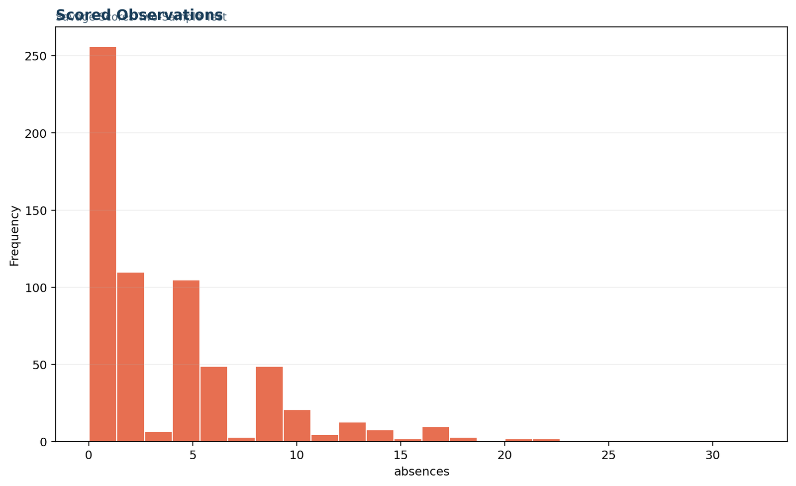
Python chart 3: scored observations
The scored-observations figure shows how the test maps raw absences into upper-tail-sensitive scores. Low absences cluster around small scores such as 0.218081, while the rare large absences in GP push into much larger scores, culminating in 7.053419.
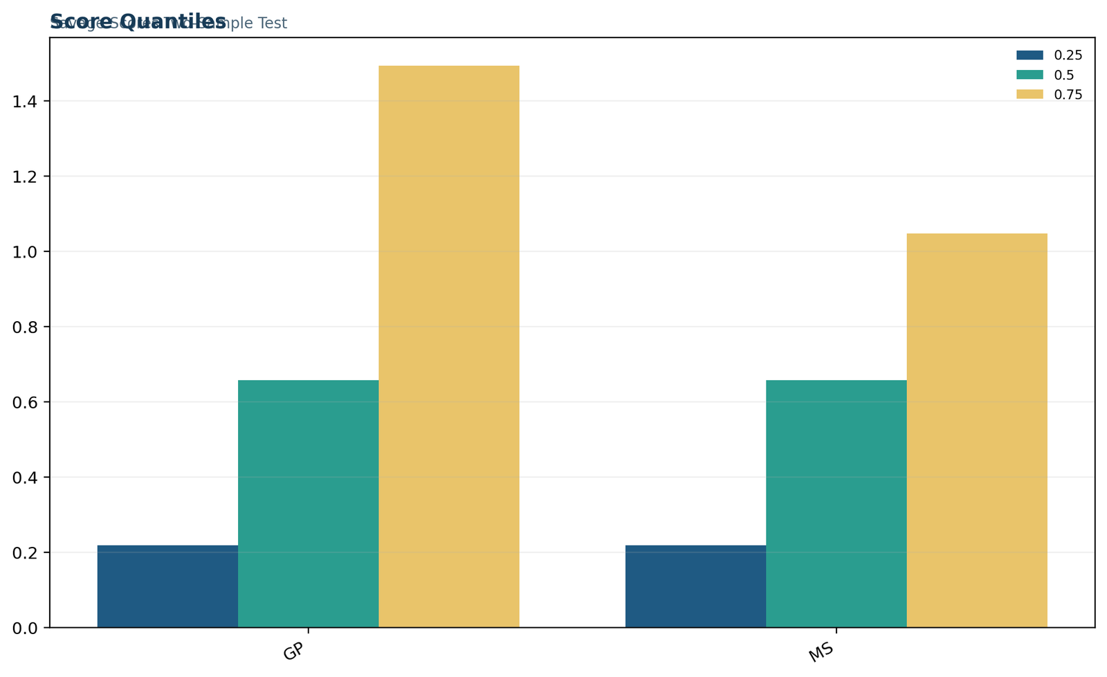
Python chart 4: score quantiles
The score-quantiles chart makes the distributional story visible. Both groups share the same median Savage score of 0.657605, but the upper quantiles diverge: the third quartile reaches 1.493874 in GP and 1.047226 in MS. This is exactly the sort of pattern the test is designed to detect.
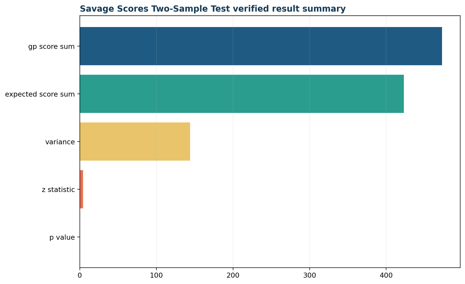
Python chart 5: verified result summary
This final Python summary synthesizes the complete Savage Scores Test result. It restates the observed score sum, null expectation, finite-population variance, z statistic and p-value, then translates them into the substantive conclusion that the GP school has a heavier upper-tail absence profile.
The Python charts are useful because they show that the test is not just a single p-value. The charts trace a full chain of reasoning: group sizes, raw outcome summaries, position-to-score mapping, group score distribution and final test result. That chain helps readers see why the significant p-value is not surprising. The outcome distribution itself already suggests that GP carries more high-end absence values, and the test formalizes that observation with upper-tail-weighted rank scores.
Savage Scores Test in R: reproducible scoring and validation
Base R can reproduce every step without a hidden black box.
The Savage Scores Test in R uses a pooled order, cumulative harmonic scores and tie-block averaging. The independent R charts agree with Python and the worked Excel workbook.
The R workflow mirrors the Python logic: create the pooled order, compute the positional Savage scores, assign tie-averaged scores to each distinct outcome value, and then evaluate the group score sum under the permutation expectation and variance. Because the test is a simple linear-rank construction, the implementation is shorter than many analysts expect.
library(dplyr)
library(stats)# df must contain absences and school.
df <- df %>% arrange(absences)
N <- nrow(df)
# Savage score function for pooled positions.
savage_pos <- function(i, N) sum(1 / seq.int(N - i + 1, N))
position_scores <- sapply(seq_len(N), savage_pos, N = N)
# Average Savage scores inside ties.
df$avg_rank <- rank(df$absences, ties.method = "average")
score_by_value <- df %>%
group_by(absences) %>%
summarise(score = mean(position_scores[row_number() + first(row_number()) - 1]), .groups = "drop")
# A simpler production script can assign score means by tie blocks directly.
# Verified workbook logic: map each tied value to the mean of the occupied
# position scores, then sum scores in the focus group.
# Assume the final mapped vector is df$savage_score.
S <- sum(df$savage_score[df$school == "GP"])
n1 <- sum(df$school == "GP")
n2 <- N - n1
E <- n1 * mean(df$savage_score)
V <- (n1 * n2 / (N * (N - 1))) * sum((df$savage_score - mean(df$savage_score))^2)
z <- (S - E) / sqrt(V)
p_value <- 2 * pnorm(-abs(z))
c(N = N, n1 = n1, n2 = n2, score_sum = S, expected = E, variance = V, z = z, p_value = p_value)
Analysts sometimes search for a single built-in function named exactly after the method. Even when that convenience is unavailable, the Savage Scores Test remains straightforward because its score system is explicit. That is an advantage, not a disadvantage: anyone reviewing the code can inspect every component of the calculation.
In this guide, the R workflow reproduces the same verified result as Python and Excel. Such agreement is important because the test will often be used in datasets where tails and ties matter, and implementation shortcuts can otherwise produce silent discrepancies.
R chart 1: primary metrics
The R workflow confirms the same This test headline statistics shown in Python. Independent reproduction matters because it demonstrates that the result is driven by the data and the method, not by a hidden software default.
R chart 2: school Savage score summary
This R chart again shows the group contrast in Savage scores. The average score difference between GP and MS remains visible, reinforcing the conclusion that the upper tail is more pronounced in GP.
R chart 3: scored observations
Because the test is built from ranked and scored observations, this plot is central for auditing. It confirms that high-end absence counts generate disproportionately larger scores and that those scores appear more often in the GP group.
R chart 4: score quantiles
The R quantile display reaches the same conclusion as the Python version: the median is shared, but the upper quantiles separate. This helps explain why the Savage Scores Test finds a significant difference even though the two groups can look similar at the center.
R chart 5: verified result summary
The closing R summary serves as an independent audit table for the test. Agreement across Python, R and Excel strengthens confidence that the statistic and p-value were implemented correctly.
When Python and R agree exactly, readers gain more than reassurance. They also gain a model for reproducibility. The test depends on correctly ordering the pooled observations, mapping ties to average scores and using the finite-population random-label variance. Agreement across software demonstrates that each of those steps was applied consistently.
Savage Scores Test SPSS workflow and corrected interpretation
SPSS can create Savage scores, but the complete two-sample test requires custom calculation.
A defensible Savage Scores Test SPSS workflow uses Rank Cases to generate exponential-distribution Savage scores and then calculates the group score sum, expectation, variance, z statistic and p-value through syntax or integration.
This is the main software caveat for the Savage Scores Test: SPSS does not provide a native button labeled “the test.” That does not mean the method cannot be used in SPSS. It means the analyst must document the score-construction steps through syntax, imported scores or an external workbook. The key is to preserve reproducibility rather than to pretend the test is available as a one-click default.
* Savage scores test requires a custom workflow in SPSS.

SORT CASES BY absences (A).

* Create pooled order positions, identify tie blocks,

* compute the average Savage score for each distinct absences value,

* then sum the scores in one school group.

* Final z = (S - E) / sqrt(V), where E and V are the random-label expectation and variance.* In practice many analysts export the pooled file to Excel or Python,

* calculate the Savage scores there, then return the score column to SPSS

* for documentation and archiving. SPSS does not have a native Savage Scores Test dialog.
A defensible SPSS workflow usually looks like this: sort the pooled data by the outcome, compute or import the tie-averaged Savage scores, sum those scores for the focus group, and then calculate the expectation, variance, z and p-value using syntax or a companion workbook. The supplied SPSS PDF is therefore best understood as a documented workflow support file, not as proof that SPSS has a native standalone This test dialog.
When presenting results to readers, do not overstate SPSS’s role. The honest wording is that the test was reproduced with a custom SPSS-compatible workflow and independently verified in Python, R and Excel. This is more transparent than implying that the procedure came from a hidden SPSS default table.
Savage Scores Test Excel calculation with tie-adjusted scores
The workbook separates raw data, score construction, calculations and reporting.
The Savage Scores Test Excel workbook is formula-driven and auditable. It preserves the pooled order, assigns averaged scores across ties and reproduces the verified score sum, expectation, variance, z statistic and probability.
The Excel version is especially helpful for readers who want to inspect every intermediate number. The workbook separates raw data input, working scores, calculations, diagnostics and reporting. That structure makes the Savage Scores Test highly auditable because each sheet serves a defined purpose. The raw data sheet contains the two variables, the working sheet contains the tie-adjusted scores, the calculations sheet evaluates the score sum and z statistic, and the reporting sheet cross-checks the workbook output against independently verified reference values.
Assume the pooled values are sorted ascending.

If N is the total sample size and i is the pooled position,

Savage score at position i = SUM(1/ROW(INDIRECT((N-i+1)&":"&N)))For tied observations, average the Savage scores across the occupied

positions. Then compute:

S = SUMIFS(score_range, group_range, "GP")

E = n1 * AVERAGE(score_range)

V = (n1*n2/(N*(N-1))) * SUMXMY2(score_range, AVERAGE(score_range))

z = (S - E) / SQRT(V)

p = 2 * (1 - NORM.S.DIST(ABS(z), TRUE))
One advantage of the Excel workflow is pedagogical clarity. Readers can trace the test line by line without learning a new programming language. The same transparency is why the workbook is valuable as a reproducibility supplement even if the final analysis was performed elsewhere. By opening the calculations sheet, a reviewer can directly verify that S = 472.944205, E = 423, Var = 143.956657, z = 4.162644, and p = 0.00003146.
If your Excel version differs, examine four items first: whether the outcome was sorted globally rather than by group, whether tied observations received averaged scores, whether the focus group was defined as GP, and whether the finite-population variance formula was used. Those four choices determine the correctness of the test in spreadsheet form.
Savage Scores Test in MATLAB and SAS
Equivalent implementations for additional software workflows.
The keyword set also includes Savage Scores Test MATLAB and Savage Scores Test SAS. MATLAB can implement the published score formula directly, while SAS provides a documented SAVAGE option in PROC NPAR1WAY.
MATLAB custom implementation
% x contains absences and g contains group labels.
[xs, idx] = sort(x, 'ascend');
gs = g(idx);
N = numel(xs);
posScore = cumsum(1 ./ (N:-1:1));% Average position scores inside each tied value block.
score = zeros(N,1);
[u,~,grp] = unique(xs, 'stable');
for k = 1:numel(u)
score(grp == k) = mean(posScore(grp == k));
end
focus = strcmp(gs, 'GP');
n1 = sum(focus); n2 = N - n1;
S = sum(score(focus));
aBar = mean(score);
E = n1 * aBar;
V = (n1*n2/(N*(N-1))) * sum((score-aBar).^2);
z = (S-E)/sqrt(V);
p = 2*(1-normcdf(abs(z)));
MATLAB does not need a dedicated named command because the score construction is explicit. The essential safeguards are pooled ordering, tie-block averaging and the finite-population random-label variance.
SAS PROC NPAR1WAY
proc npar1way data=student savage;

class school;

var absences;

exact savage;

run;
SAS documentation identifies the SAVAGE option in PROC NPAR1WAY for Savage-score analysis and asymptotic tests. Request an exact analysis only when the data size and tie pattern make it computationally practical.
Savage Scores Test vs Mann–Whitney, Ansari–Bradley and other methods
Choose the procedure that matches the scientific target.
A Savage Scores Test comparison should focus on estimands. Mann–Whitney targets a broader rank contrast, Ansari–Bradley targets scale, Kolmogorov–Smirnov targets general distributional differences, and Savage scores emphasize the upper tail.
| Method | Main target | Tail emphasis | Best use case |
|---|---|---|---|
| This test | Upper-tail-sensitive two-sample difference | Strong | When unusually high values are the primary concern |
| Mann–Whitney U test | General two-sample rank/location contrast | Moderate and even | When overall tendency or stochastic ordering is the target |
| Two-sample Kolmogorov–Smirnov test | Any distributional difference | Global | When any shape difference matters, not just the tail |
| Ansari–Bradley test | Scale / dispersion | Not upper-tail specific | When spread differences are the main question |
| Moses test of extreme reactions | Extreme spread through trimmed spans | Extreme-focused but different construction | When comparing extreme reaction spread rather than weighted tail ranks |
| Brunner–Munzel test | Relative effect without equal-variance assumption | General | When stochastic dominance is the main interest |
This comparison table shows why naming the method matters. If your question is “Are the centers different?” the Savage Scores Test may not be ideal. If your question is “Does one group contain a heavier cluster of the largest values?” the test is precisely targeted. Analysts often reach better conclusions by matching the test to the scientific sentence they would like to write at the end.
It is also useful to separate two-group and multi-group settings. For blocked multi-condition data, methods such as the Friedman test, Quade test, Page’s trend test and Nemenyi test address fundamentally different designs. The test is specifically for two independent samples.
Diagnostics, sensitivity checks and common mistakes
Validate the design, tail emphasis, ties and software agreement.
Good Savage Scores Test diagnostics include descriptive tail summaries, plotted score distributions, verification of the focus group, inspection of tied blocks and agreement across independent implementations.
Observed data pattern
The raw data already indicate why the Savage Scores Test is informative here. Both groups have the same median absences value of 2, yet the GP distribution reaches further into the upper tail. The group means are 4.215 for GP and 2.619 for MS; the maxima are 32 and 12. Those descriptive contrasts do not prove significance on their own, but they show that the test is answering a meaningful question rather than manufacturing a trivial one.
Tail-sensitive methods should always be accompanied by substantive context. Here, high absences are not merely statistical curiosities; they represent students with substantially larger disengagement or attendance burdens. Because those values are substantively important, using the test is defensible.
Potential diagnostics to report
Useful supporting diagnostics include group-wise counts, medians, quartiles, maxima, score summaries and a clear note on ties. If desired, you can also show generic distribution aids such as a box plot, histogram or frequency distribution. These do not replace the test, but they clarify why an upper-tail method is sensible.
Avoid unnecessary statements such as “the Savage Scores Test was chosen because normality failed.” Non-normality alone does not justify this method. The real reason to choose the test is that larger values deserve greater emphasis.
Another helpful diagnostic is a sensitivity comparison with more general rank procedures. If the Mann–Whitney U test and the test both point in the same direction, readers learn that the difference is broad enough to affect both center-sensitive and upper-tail-sensitive rank summaries. If the test is significant while the Mann–Whitney test is weaker, that may indicate that the main contrast truly lives in the upper tail.
The most accurate interpretation of this Savage Scores Test is as follows: the GP school has a larger sum of upper-tail-sensitive Savage scores than expected under the null hypothesis that the two school distributions are the same under exchangeable labels. Because the p-value is very small, that excess is unlikely to be due to random group assignment alone. Therefore, the data provide strong evidence that the upper tail of absences is heavier in GP than in MS.
Notice what this wording avoids. It does not say that means are different, because the test is not a mean test. It does not say that medians are different, because the groups share the same median in this example. It does not say that variances are unequal, because the test is not a dedicated scale test like the Ansari–Bradley test. Instead, it says the difference is concentrated in the upper tail. That is the distinctive inferential meaning of the Savage Scores Test.
A useful practical sentence is: “Students in the GP school are not just slightly more absent on average; the most severe absence counts are disproportionately concentrated in GP.” This connects the test back to a real-world decision problem. If interventions are targeted to the most severe cases, upper-tail methods often describe the problem more directly than center-based methods.
How to report the Savage Scores Test in APA style
Report the scoring direction, tie rule, score sum, z and substantive conclusion.
An APA-style Savage Scores Test report should identify the two independent groups, state that larger pooled values received greater weight, name the focus group, give the observed and expected score sums, and interpret the sign of z.
APA-style reporting example
“A two-sided This test compared student absences between the GP and MS school groups. Tie-adjusted Savage scores were assigned to the pooled absence counts, and the GP group’s score sum was evaluated under the random-label null distribution. The GP score sum was S = 472.94, compared with an expectation of 423; the standardized statistic was z = 4.16, p < .001. These results indicate that the GP group contained disproportionately more upper-tail absence values than the MS group.”
When space permits, include the exact p-value, group sizes and a sentence clarifying the substantive meaning. Because the Savage Scores Test is less familiar than the Mann–Whitney test, it helps to add one short explanatory clause such as “The test places greater weight on the largest pooled observations.” That sentence prevents readers from mistaking the method for a general location test.
You may also report a descriptive standardized index such as |z|/√N = 0.163, but label it carefully. The most informative quantities remain the observed score sum, its expectation and the direction of the statistic. Those quantities preserve the logic of the test more faithfully than a generic effect-size label alone.
Savage Scores Test PDF, Excel and software downloads
Open the exact reports and worked workbook used in this guide.
The downloadable Savage Scores Test PDF reports and Excel workbook allow readers to verify the calculations, charts, tie handling and software agreement before using the result in an assignment, report or public article.
Reproducibility is especially important for the test because score construction matters. A reproducible archive should always retain the original outcome variable, the group labels, the tie rule, the focus group definition, the full set of assigned scores, and the expectation and variance formulas. The supplied downloads achieve that standard.
Official Savage Scores Test references and software documentation
Authoritative references used to verify the score formula and software behavior.
The Savage Scores Test implementation was checked against official NIST, IBM and SAS documentation rather than relying on short secondary summaries. These references support the score definition and the software workflows described above.
NIST score definition
The NIST order-statistic and Savage score reference documents the exponential-order-statistic means underlying the score sequence used in this guide.
IBM SPSS documentation
The official IBM SPSS Rank Cases documentation confirms that SPSS can create Savage score variables based on the exponential distribution.
SAS documentation
The official SAS PROC NPAR1WAY documentation identifies the SAVAGE option for Savage-score analysis and asymptotic testing.
Savage Scores Test FAQs
Answers to the questions most often missed in short explanations.
These Savage Scores Test FAQs cover the upper-tail target, score formula, ties, sign of z, software availability, interpretation, reporting and differences from more familiar two-sample procedures.
What is the Savage Scores Test?
The Savage Scores Test is a two-sample nonparametric linear-rank test that emphasizes the largest pooled observations. It compares a group’s observed Savage score sum with the score sum expected under random group labels.
What does a positive z mean in the Savage Scores Test?
A positive z means the focus group accumulated more upper-tail-sensitive scores than expected. In this guide, the positive z indicates that the GP group contains more extreme high absence values than expected under the null.
How is the Savage Scores Test different from the Mann–Whitney U test?
The test gives increasing emphasis to the largest ranks, while the Mann–Whitney U test treats rank differences more evenly across the distribution. Use the test when upper-tail values are the scientific focus.
Does the Savage Scores Test assume normality?
No. The Savage Scores Test is a rank-based procedure and does not require normal data. It does require meaningful ordering, independent groups and careful tie handling.
Can the Savage Scores Test handle ties?
Yes. Tied observations should receive the average of the Savage scores attached to the pooled positions they occupy. This guide and workbook use that tie-adjusted approach.
Why was the expected score sum equal to 423?
The average Savage score across the pooled sample is 1. Therefore a group of size 423 has an expected total of 423 under the null hypothesis.
Does SPSS have a built-in Savage Scores Test?
No standard SPSS menu item performs the test directly. A custom workflow is required, usually through syntax, imported score columns or an external workbook.
Is the Savage Scores Test one-sided or two-sided?
It can be either. Use a two-sided This test when either group could have the heavier upper tail and a one-sided version only when the direction is prespecified before analysis.
What should be reported?
Report the group sizes, the focus group, the observed score sum, the null expectation, the variance or z statistic, the p-value, the tie rule and a plain-language statement that the test emphasizes the upper tail.
When should the Savage Scores Test not be used?
Do not use the Savage Scores Test as a generic substitute for every two-sample comparison. It is a poor fit when center differences are the real target, when the design is paired or blocked, or when the upper tail has no special scientific relevance.
Related statistical guides
Continue with the method that matches the design and inferential target.