
Adjusted Means, G1 Covariate, School × Sex Interaction and Partial Eta Squared
Two Way ANCOVA: Formula, Interpretation, SPSS, Python, R and Excel Guide
Two Way ANCOVA tests whether a continuous outcome differs across two categorical factors after adjusting for one or more covariates. In this worked Salar Cafe example, the outcome is G3 final grade, the two factors are school and sex, and the covariate is G1. After controlling for G1, the ANCOVA shows significant school and sex effects, while the school × sex interaction is not significant.
Quick Answer: Two Way ANCOVA Result
The worked Two Way ANCOVA compares adjusted G3 means for school and sex after controlling for G1. The covariate is extremely important in this model because earlier grade performance strongly predicts final grade.
The Python summary table reports that G1 is significant, F = 1200, p = 2.77e-149, partial η² = 0.6508. After this covariate adjustment, school remains significant, F = 5.136, p = 0.02377, partial η² = 0.007912. Sex is also significant, F = 4.93, p = 0.02674, partial η² = 0.007598. The school × sex interaction is not significant, F = 0.0006807, p = 0.9792.
The SPSS output confirms the same decision pattern. The Type III ANCOVA table reports G1 p < .001, school p = .027, sex p = .036, and school × sex p = .979. The corrected model explains a large amount of variation, with R² = .687 and adjusted R² = .685.
Final interpretation: After controlling for G1, adjusted G3 differs by school and sex. Female students have higher adjusted means than male students in both schools, and GP remains higher than MS after adjustment. The school × sex interaction is not significant, so the difference between female and male students is not meaningfully different across schools.
Important reporting point: Two Way ANCOVA is not the same as Two Way ANOVA. ANCOVA compares adjusted means after controlling for a covariate. In this example, raw school and sex means are reduced after controlling for G1, showing why covariate adjustment matters.
Table of Contents
- What Is Two Way ANCOVA?
- Two Way ANCOVA Formula
- Two Way ANCOVA Hypotheses
- Dataset and Variables Used
- Two Way ANCOVA Assumptions
- SPSS Output Interpretation
- Python Chart-by-Chart Interpretation
- R Chart-by-Chart Validation
- SPSS, R, Python and Excel Workflows
- Code Blocks for Two Way ANCOVA
- APA Reporting Wording
- Common Mistakes
- When to Use Two Way ANCOVA
- Downloads and Resources
- Related Guides
- FAQs
What Is Two Way ANCOVA?
Two Way ANCOVA is an analysis of covariance model with one numeric dependent variable, two categorical independent variables and at least one numeric covariate. It combines the group-comparison logic of Factorial ANOVA with the covariate-adjustment logic of ANCOVA.
In a standard One Way ANOVA, group means are compared directly. In Two Way ANCOVA, group means are compared after adjusting for a covariate. In this example, G1 is the covariate because earlier grade performance is strongly related to G3 final grade. The model asks whether school and sex still matter after G1 is controlled.
The result shows that G1 explains the largest share of G3 variation. However, school and sex still show statistically significant adjusted effects. The interaction between school and sex is almost zero and not significant, which means the school difference does not meaningfully depend on sex and the sex difference does not meaningfully depend on school.
Simple definition: Two Way ANCOVA compares adjusted group means for two factors after controlling for a covariate. Here, it compares adjusted G3 means for school and sex after controlling for G1.
This guide connects naturally with One Way ANCOVA, ANOVA Assumptions, ANOVA Effect Size, Eta Squared, Omega Squared, F Distribution, ANOVA in SPSS, ANOVA in R and ANOVA in Python.
Two Way ANCOVA Formula
A two-factor ANCOVA model includes the covariate, the two main effects, the two-way interaction and the residual error term. The model can be written as:
In this formula, Y is the dependent variable, A is the first factor, B is the second factor, AB is the interaction, X is the covariate, and β is the covariate slope. In this example, Y is G3, A is school, B is sex and X is G1.
F Statistic Formula
Each ANCOVA effect has its own F statistic. The covariate has an F test, each main effect has an F test, and the interaction has an F test. A significant F test means that the effect explains variation in G3 after the other model terms are considered.
Partial Eta Squared Formula
Partial eta squared shows the practical size of each adjusted effect. In this model, the covariate G1 has a very large effect, with partial eta squared around 0.651. School and sex are statistically significant but much smaller, with partial eta squared values around 0.008. The school × sex interaction is essentially zero.
| Effect | df | F | p | Partial η² | Decision | Interpretation |
|---|---|---|---|---|---|---|
| G1 | 1 | 1200 | 2.77e-149 | 0.6508 | Reject H0 | Very strong covariate effect. |
| school | 1 | 5.136 | 0.02377 | 0.007912 | Reject H0 | Adjusted G3 differs by school. |
| sex | 1 | 4.93 | 0.02674 | 0.007598 | Reject H0 | Adjusted G3 differs by sex. |
| school × sex | 1 | 0.0006807 | 0.9792 | 0.000001 | Fail to reject H0 | No adjusted interaction evidence. |
Two Way ANCOVA Hypotheses
Two Way ANCOVA has separate hypotheses for the covariate, each main effect and the interaction. The interaction should be interpreted before over-explaining the main effects.
| Effect | Null Hypothesis | Alternative Hypothesis | Decision in This Output |
|---|---|---|---|
| G1 covariate | G1 does not predict G3 after school and sex are included. | G1 predicts G3 after school and sex are included. | Reject H0. |
| school | Adjusted mean G3 is equal for GP and MS. | Adjusted mean G3 differs by school. | Reject H0. |
| sex | Adjusted mean G3 is equal for female and male groups. | Adjusted mean G3 differs by sex. | Reject H0. |
| school × sex | The adjusted school difference is the same across sex groups. | The adjusted school difference depends on sex. | Fail to reject H0. |
Decision for this example: G1, school and sex are statistically significant. The school × sex interaction is not significant. The final interpretation should focus on adjusted main effects, not on interaction storytelling.
Dataset and Variables Used
The worked example uses student performance data. The dependent variable is G3 final grade. The covariate is G1. The two categorical factors are school and sex. The SPSS output includes 649 valid cases.
| Variable | Role | Levels / Type | Why It Matters |
|---|---|---|---|
| G3 | Dependent variable | Numeric final grade | The outcome being compared after adjustment. |
| G1 | Covariate | Numeric earlier grade | Controls for prior academic performance. |
| school | Factor A | GP, MS | Tests adjusted school difference. |
| sex | Factor B | F, M | Tests adjusted sex difference. |
| school × sex | Interaction | Four cells | Tests whether the school effect depends on sex. |
Raw Cell Means Before Covariate Adjustment
| school | sex | N | Raw G3 Mean | Raw G1 Mean | Interpretation |
|---|---|---|---|---|---|
| GP | F | 237 | 13.0042 | 12.2869 | Highest raw G3 cell mean. |
| GP | M | 186 | 12.0323 | 11.6022 | Lower than GP female but still above MS groups. |
| MS | F | 146 | 11.0342 | 10.5822 | Higher than MS male. |
| MS | M | 80 | 9.9500 | 9.7875 | Lowest raw G3 cell mean. |
| Total | F | 383 | 12.2533 | 11.6371 | Female raw mean is higher overall. |
| Total | M | 266 | 11.4060 | 11.0564 | Male raw mean is lower overall. |
The raw cell means show a strong pattern before adjustment: GP students have higher G3 means than MS students, and female students have higher G3 means than male students. ANCOVA then checks whether these differences remain after controlling for G1.
For supporting concepts, review Descriptive Statistics, Mean Median and Mode, Standard Deviation, Variance, Confidence Interval, P Value and Null and Alternative Hypothesis.
Two Way ANCOVA Assumptions
Two Way ANCOVA has the usual ANOVA assumptions plus additional covariate assumptions. The most important extra idea is that the covariate should have a reasonably linear relationship with the outcome and the covariate slope should be comparable across groups.
| Assumption | What It Means | How This Example Checks It |
|---|---|---|
| Continuous outcome | Dependent variable should be numeric. | G3 is a numeric final grade. |
| Categorical factors | Independent variables should define groups. | school and sex define four cells. |
| Covariate measured before or independently | Covariate should not be an outcome caused by the factor treatment. | G1 is an earlier grade used to adjust G3. |
| Linearity | Covariate should relate linearly to the outcome. | The G1 versus G3 scatterplot shows a strong positive relationship. |
| Homogeneity of regression slopes | The covariate slope should be reasonably similar across groups. | Group-specific trend lines should be reviewed before final reporting. |
| Homogeneity of error variance | Residual variance should be reasonably similar across cells. | SPSS Levene test reports p = .119, supporting no serious variance violation. |
| Residual diagnostics | Residuals should be approximately normal and randomly scattered. | Residual and Q-Q plots show usable model fit with visible tail departures. |
For deeper assumption checks, use Levene Test, Bartlett’s Test, Q-Q Plot Normality Check, P-P Plot Normality Check, Shapiro-Wilk Test, Studentized Residuals, Cook’s Distance and Outlier Detection.
SPSS Output Interpretation for Two Way ANCOVA
The SPSS output uses UNIANOVA with G3 as the dependent variable, school and sex as fixed factors, and G1 as the covariate. The model is written as G3 = G1 + school + sex + school × sex.
SPSS Reading Order
| SPSS Output Area | What to Read | Why It Matters |
|---|---|---|
| Between-subject factors | school_id and sex_id levels. | Confirms GP/MS and F/M grouping. |
| Descriptive statistics | Raw G3 means for school × sex cells. | Shows the unadjusted pattern. |
| Levene test | F = 1.960, p = .119. | Checks equality of error variances. |
| Tests of between-subject effects | G1, school, sex and school × sex rows. | Main ANCOVA decision table. |
| Partial eta squared | Effect-size column. | Shows practical strength after adjustment. |
| Parameter estimates | G1 slope and group estimates. | Shows direction of covariate and group coding effects. |
SPSS Type III ANCOVA Table
| Source | Type III SS | df | MS | F | Sig. | Partial η² | Interpretation |
|---|---|---|---|---|---|---|---|
| Corrected Model | 4648.278 | 4 | 1162.069 | 353.842 | < .001 | .687 | The full model is significant. |
| G1 | 3942.442 | 1 | 3942.442 | 1200.448 | < .001 | .651 | G1 is the dominant covariate. |
| school | 16.081 | 1 | 16.081 | 4.897 | .027 | .008 | Adjusted G3 differs by school. |
| sex | 14.492 | 1 | 14.492 | 4.413 | .036 | .007 | Adjusted G3 differs by sex. |
| school × sex | .002 | 1 | .002 | .001 | .979 | .000 | No adjusted interaction. |
| Error | 2114.989 | 644 | 3.284 | Residual error term. |
SPSS Descriptive Pattern
The SPSS descriptive table shows that GP female students have the highest raw G3 mean at about 13.00, while MS male students have the lowest raw G3 mean at about 9.95. The total female mean is about 12.25, and the total male mean is about 11.41.
After controlling for G1, the adjusted means are closer together than the raw means, but the school and sex effects remain statistically significant. This is the central ANCOVA message: the group differences are smaller after adjustment, yet still detectable.
SPSS interpretation summary: The ANCOVA model is significant, R² = .687, adjusted R² = .685. G1 is a strong covariate, F(1, 644) = 1200.448, p < .001, partial η² = .651. School is significant, F(1, 644) = 4.897, p = .027, partial η² = .008. Sex is significant, F(1, 644) = 4.413, p = .036, partial η² = .007. The school × sex interaction is not significant, F(1, 644) = .001, p = .979.
Python Chart-by-Chart Interpretation
The Python chart sequence explains Two Way ANCOVA through adjusted means, covariate relationship, p-value decisions, partial eta squared, raw cell means and residual diagnostics.
Python Chart 1: Adjusted Means by School and Sex
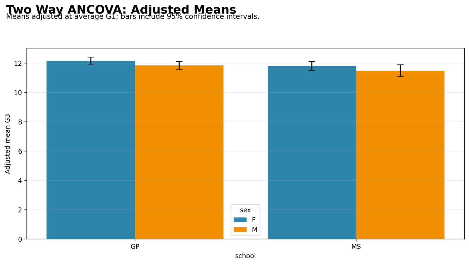
The adjusted mean chart shows GP higher than MS after covariate adjustment. Within both schools, female students have higher adjusted G3 means than male students.
The adjusted means are closer together than the raw means, which shows the effect of controlling for G1. The chart supports significant school and sex main effects but does not show a meaningful school × sex interaction.
Python Chart 2: Covariate Relationship Between G1 and G3
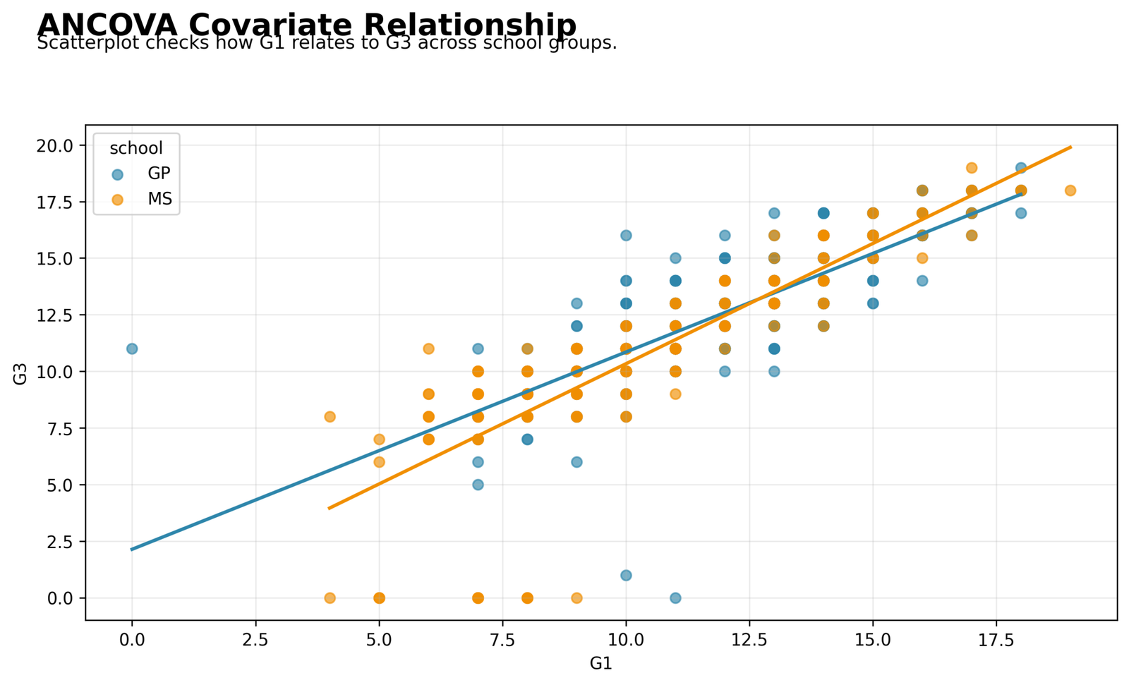
The covariate plot shows a strong positive relationship between G1 and G3. Students with higher G1 scores generally have higher G3 scores. This explains why G1 has the largest partial eta squared in the ANCOVA model.
The school trend lines both rise, but they should be reviewed as part of the homogeneity of regression slopes assumption. The main model adjusts G3 at the average G1 level, so the covariate relationship is central to the analysis.
Python Chart 3: ANCOVA Effect p-values
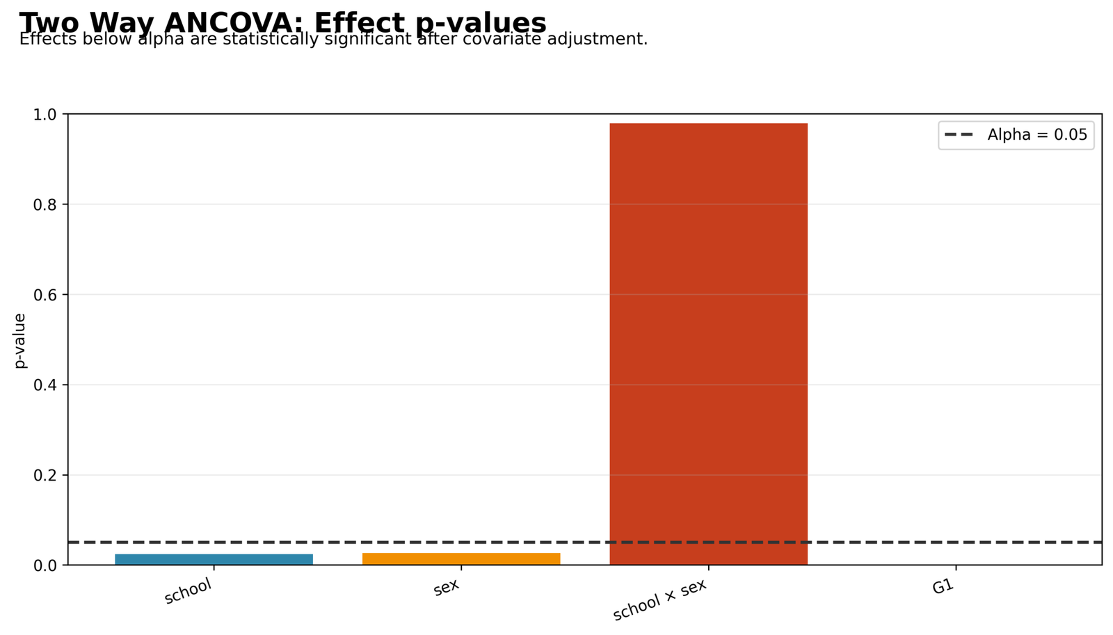
The p-value chart shows that school, sex and G1 fall below the alpha = .05 line. The school × sex interaction is far above alpha.
This chart gives the main decision visually. The covariate is significant, both main effects are significant, and the interaction should not be interpreted as meaningful.
Python Chart 4: Partial Eta Squared by Effect
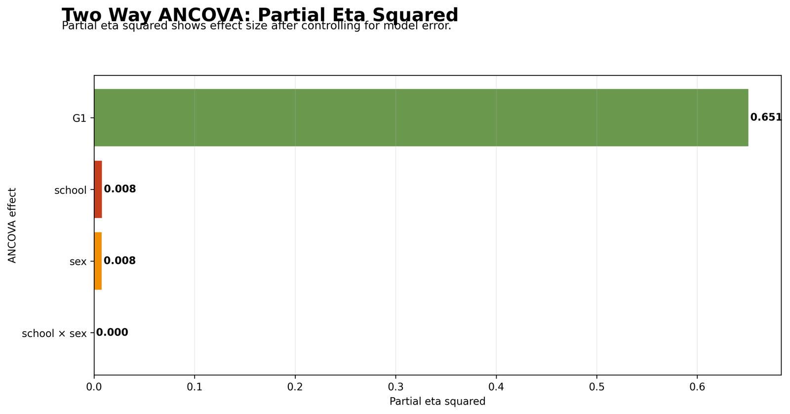
The effect-size chart shows that G1 dominates the model with partial eta squared around 0.651. School and sex are much smaller, each around 0.008.
This means the final report should separate statistical significance from practical size. G1 is the major explanatory variable, while school and sex are significant but small adjusted effects.
Python Chart 5: Raw Cell Means Before Covariate Adjustment
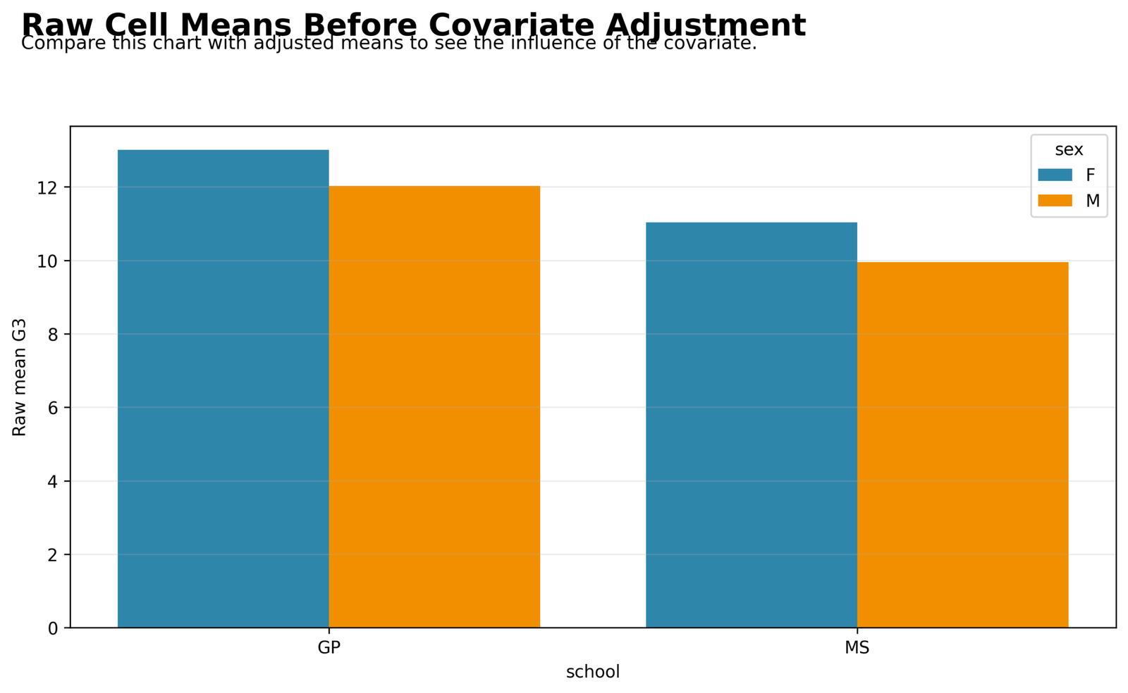
The raw mean chart shows wider group separation before covariate adjustment. GP female students have the highest raw mean, and MS male students have the lowest raw mean.
When this chart is compared with the adjusted means chart, the influence of G1 becomes clear. Covariate adjustment narrows the differences, but it does not remove the school and sex effects completely.
Python Chart 6: Residuals vs Fitted Values
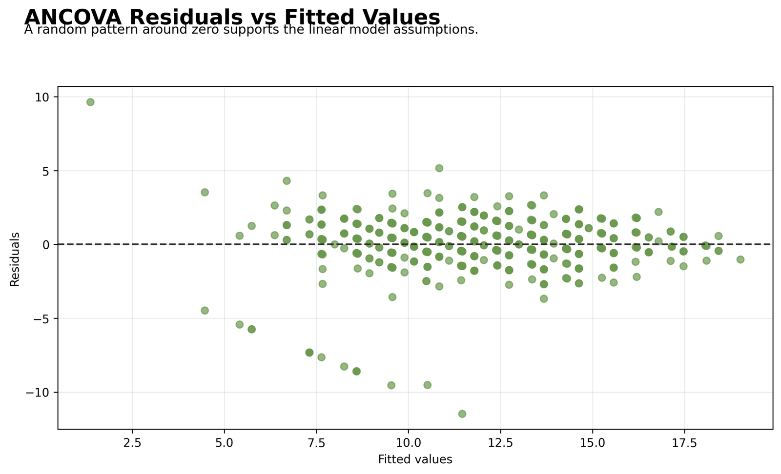
The residual plot shows most residuals scattered around zero across the fitted-value range. This supports the basic linear-model structure of the ANCOVA.
Some large negative residuals are visible, and one high positive residual appears on the left side. These points should be mentioned as diagnostic context, especially when writing a transparent assumptions section.
Python Chart 7: Residual Q-Q Plot
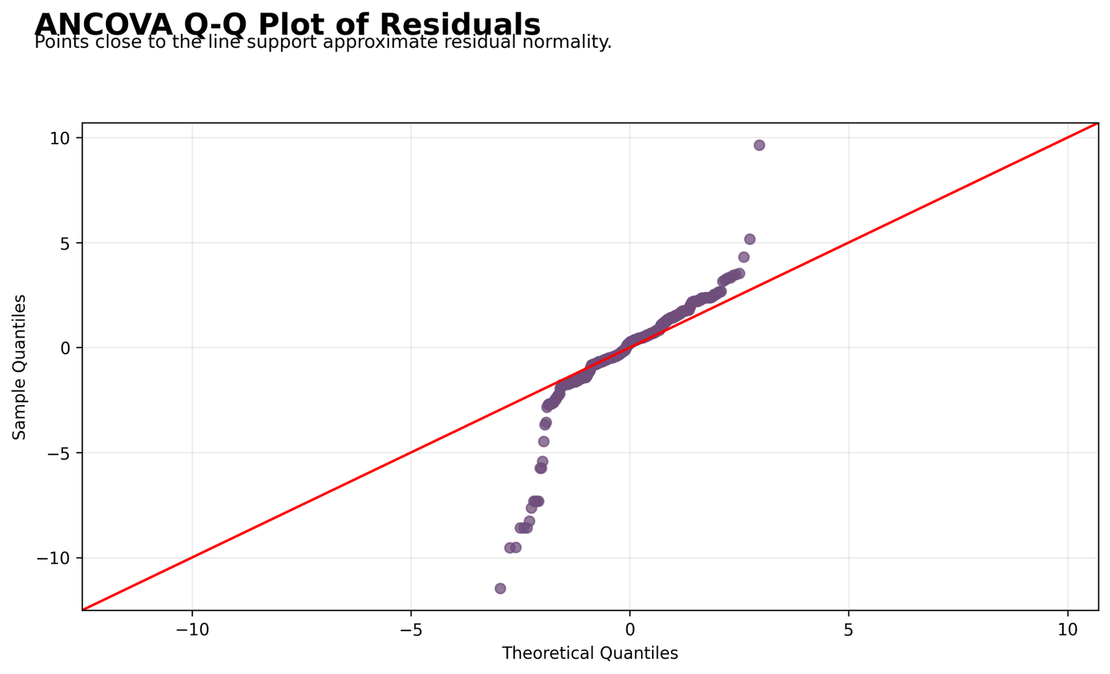
The Q-Q plot shows that the middle residuals are closer to the reference line than the tails. The lower tail departs strongly from the line.
This means residual normality is approximate rather than perfect. With a large sample, the ANCOVA results can still be reported, but the lower-tail departure should be described honestly.
Python Chart 8: ANCOVA Summary Table
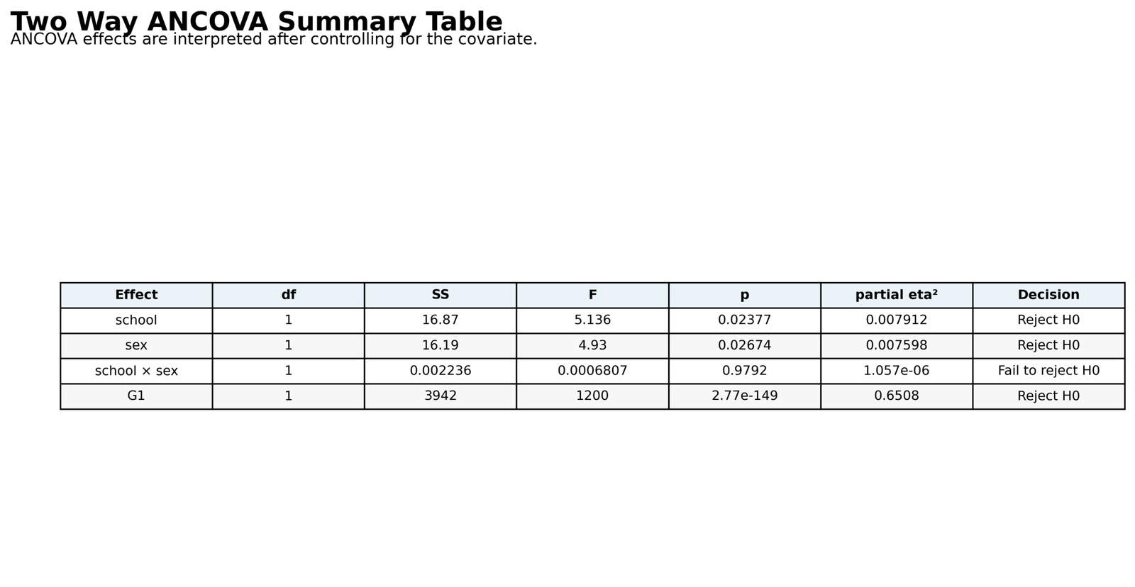
The summary table confirms the final decision. G1, school and sex are significant, while school × sex is not significant.
This is the best Python table for final reporting because it gives the formal model effects, p-values, effect sizes and decisions in one place.
R Chart-by-Chart Validation
The R validation charts repeat the same ANCOVA workflow in a second software environment. The R images confirm the same decision pattern: G1 is the strongest effect, school and sex are significant adjusted effects, and the school × sex interaction is not significant.
R Chart 1: Adjusted Means by School and Sex
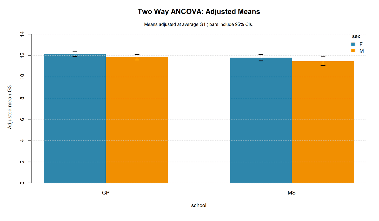
The R adjusted mean chart confirms the same pattern as Python. GP remains above MS, and female students remain above male students after controlling for G1.
This software agreement strengthens the adjusted main-effect interpretation.
R Chart 2: Covariate Relationship
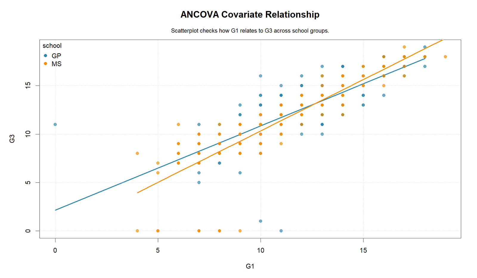
The R scatterplot confirms the strong positive relationship between G1 and G3. Higher G1 scores generally correspond to higher G3 scores.
This validates why G1 must be included as a covariate instead of comparing raw group means only.
R Chart 3: ANCOVA Effect p-values
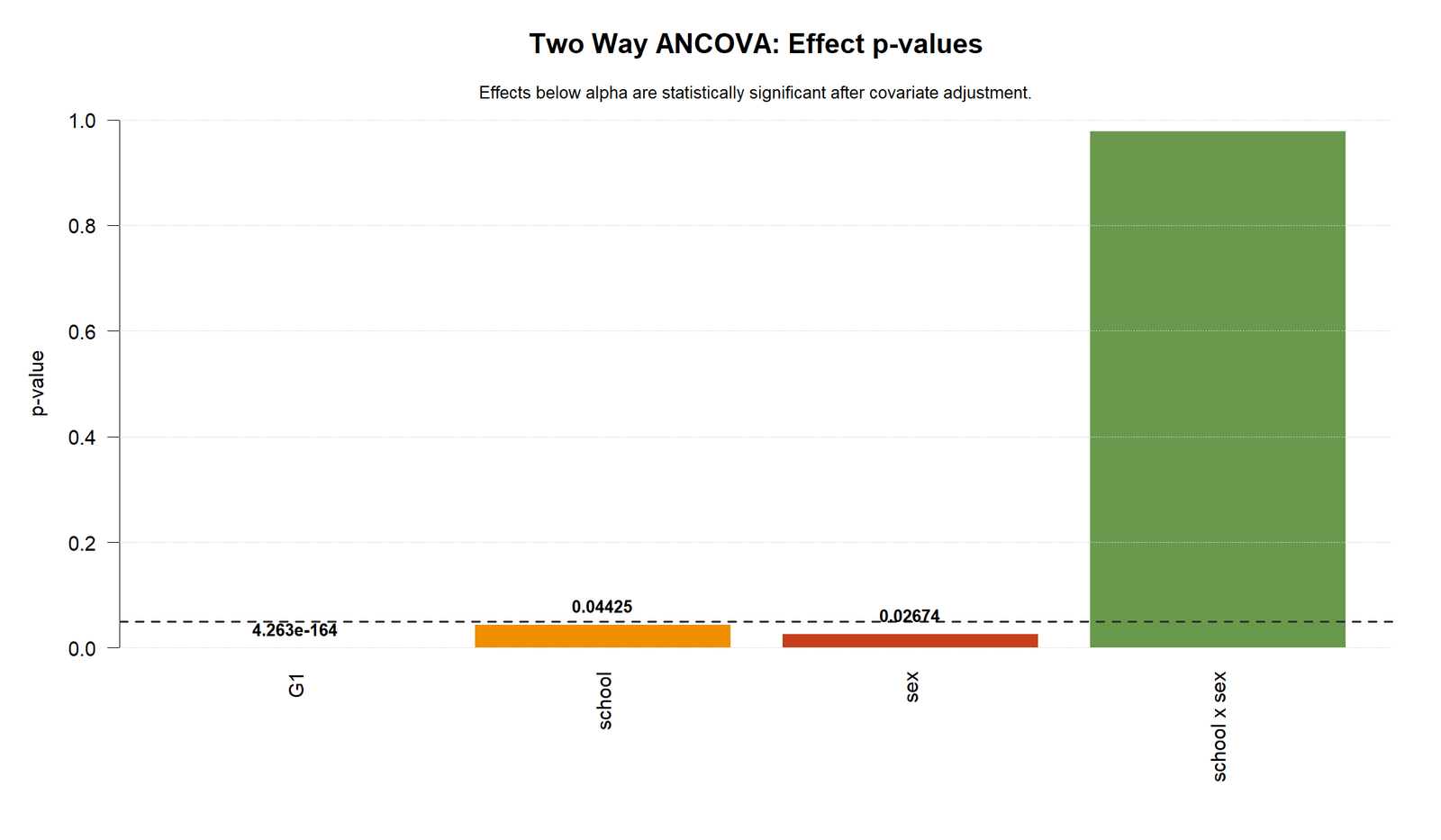
The R p-value chart confirms the same decision structure: G1, school and sex are significant, while the interaction is not significant.
This supports a final report focused on adjusted main effects rather than interaction explanation.
R Chart 4: Partial Eta Squared by Effect
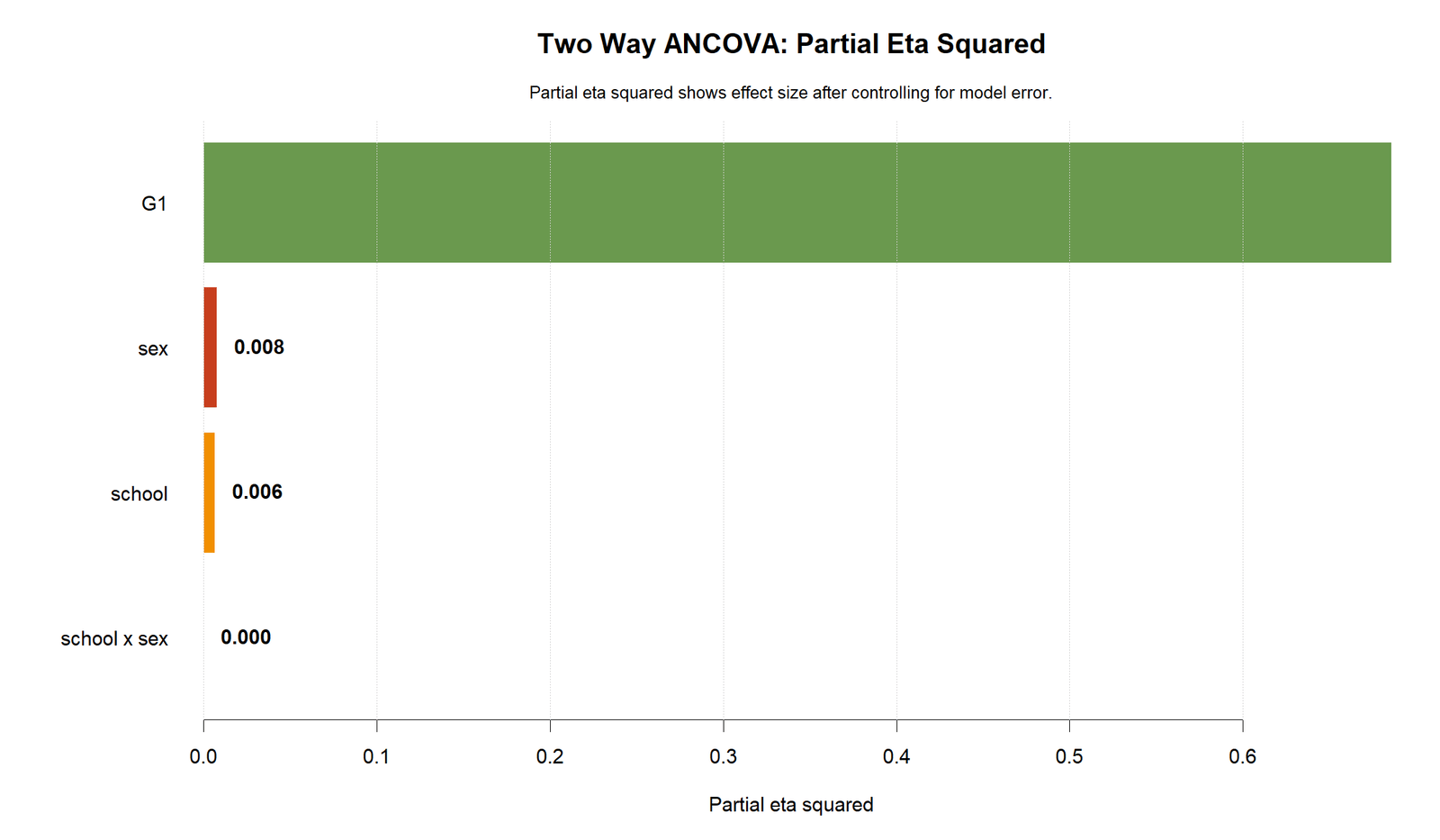
The R effect-size chart confirms that G1 has the dominant practical effect. School and sex are much smaller.
This helps prevent overstatement. The group effects are statistically significant, but G1 explains most of the adjusted variation.
R Chart 5: Raw Cell Means Before Adjustment
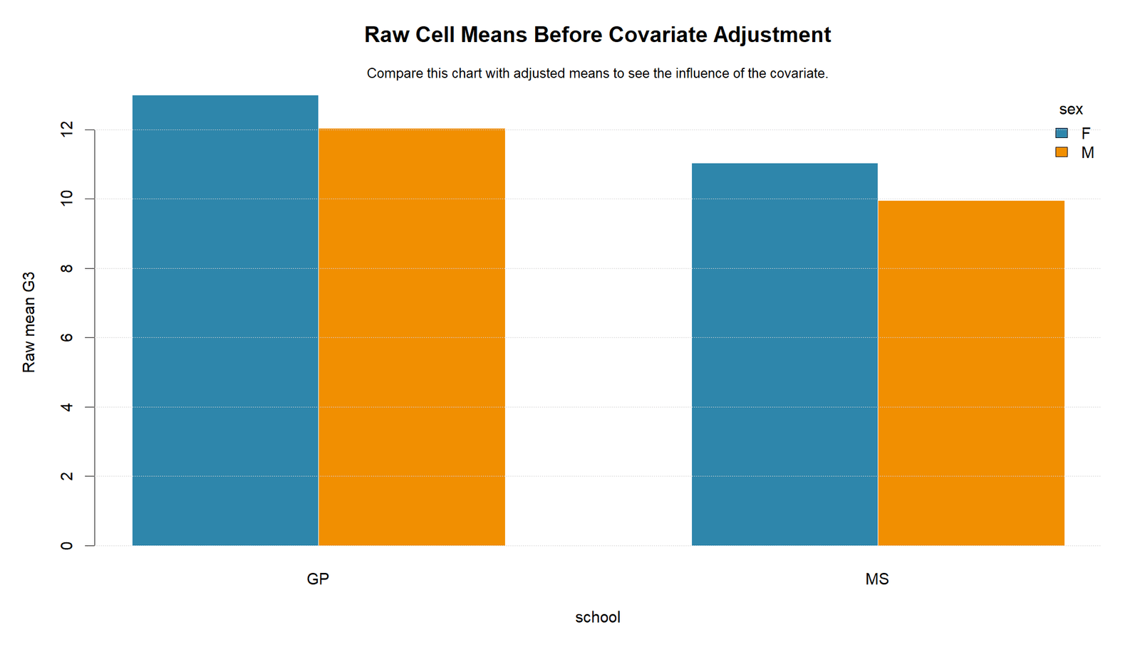
The R raw mean chart confirms that raw group differences are larger before G1 adjustment.
This validates the ANCOVA logic: raw means are useful descriptively, but adjusted means are the correct focus of interpretation.
R Chart 6: Residuals vs Fitted Values
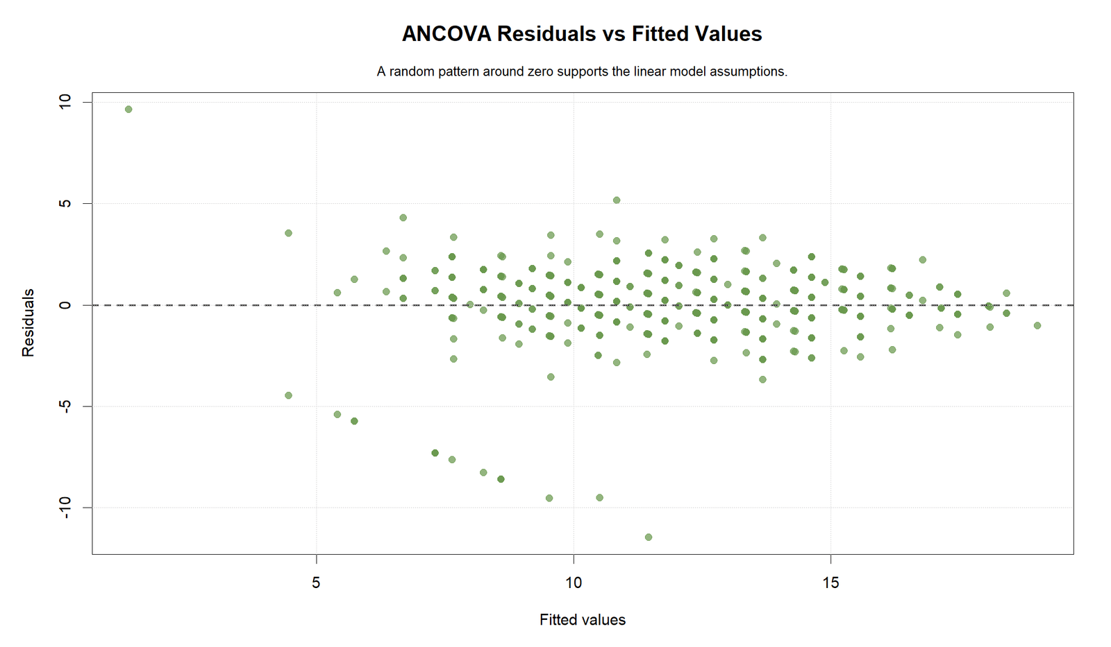
The R residual plot confirms the same diagnostic message as Python. Most residuals are centered around zero, while some lower-tail residuals remain visible.
The model is useful for adjusted mean comparison, but diagnostics should be reported with caution about extreme residuals.
R Chart 7: Residual Q-Q Plot
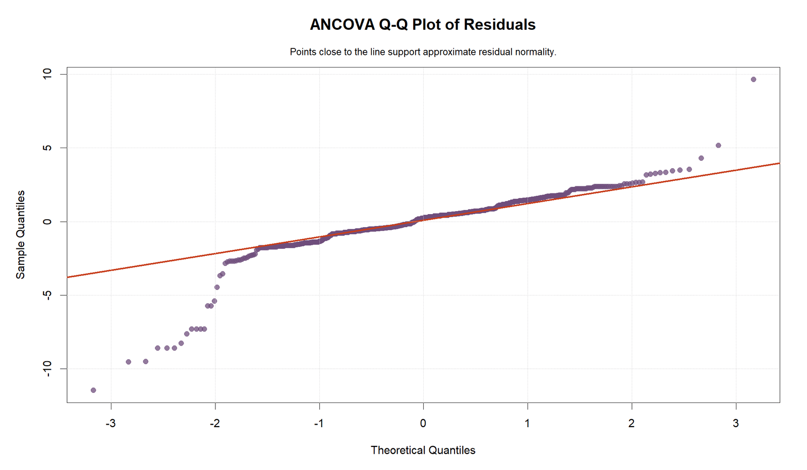
The R Q-Q plot confirms that residual normality is approximate. The lower tail departs from the reference line.
This supports a transparent diagnostic statement in the final report.
R Chart 8: ANCOVA Summary Table
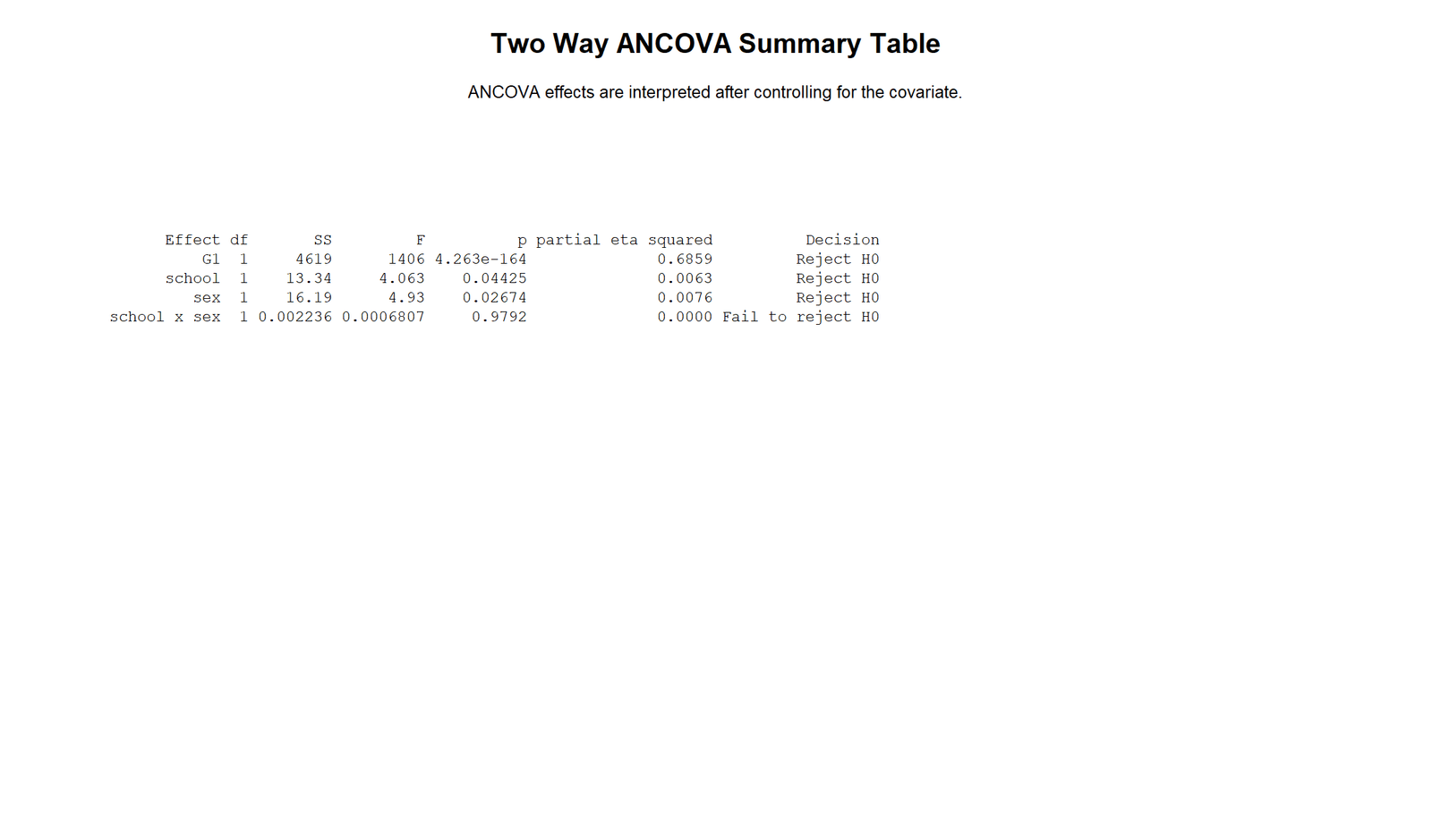
The R summary table confirms the same final interpretation. G1 is strongly significant, school and sex are significant, and school × sex is not significant.
The R table may show small numerical differences from the Python table because of implementation and table-format choices, but the statistical decisions are the same.
SPSS, R, Python and Excel Workflows for Two Way ANCOVA
The same Two Way ANCOVA workflow can be reproduced in SPSS, R, Python and Excel. SPSS uses the General Linear Model univariate procedure. R and Python use linear-model syntax with categorical factors and a covariate. Excel can prepare adjusted summaries and visuals, but SPSS, R or Python is recommended for the full ANCOVA table.
SPSS Workflow
| Step | SPSS Menu or Syntax | Purpose |
|---|---|---|
| Open data | File > Open > Data | Load G3, G1, school and sex. |
| Open ANCOVA procedure | Analyze > General Linear Model > Univariate | Run ANCOVA as a univariate GLM. |
| Set outcome | Dependent Variable: G3 | Define the final grade outcome. |
| Set fixed factors | school and sex | Define the two categorical factors. |
| Set covariate | G1 | Control earlier grade performance. |
| Choose full model | G1 + school + sex + school × sex | Test adjusted main effects and interaction. |
| Request output | Descriptives, effect size, homogeneity | Get means, partial eta squared and Levene test. |
| Export output | OUTPUT EXPORT | Save SPSS output PDF. |
R Workflow
| Step | R Action | Purpose |
|---|---|---|
| Read data | read.csv("dataset.csv") | Load the dataset. |
| Convert factors | factor(school), factor(sex) | Define categorical variables. |
| Fit model | lm(G3 ~ G1 + school * sex) | Run the ANCOVA model. |
| ANOVA table | anova(model) or car::Anova() | Get effect tests. |
| Adjusted means | emmeans::emmeans() | Estimate adjusted group means. |
| Diagnostics | Residual and Q-Q plots | Check assumptions. |
Python Workflow
| Step | Python Action | Purpose |
|---|---|---|
| Read data | pandas.read_csv() | Load G3, G1, school and sex. |
| Fit OLS model | G3 ~ G1 + C(school) * C(sex) | Run the two-way ANCOVA model. |
| ANOVA table | anova_lm(model, typ=2) | Get F values and p-values. |
| Effect sizes | Calculate partial eta squared | Report practical size. |
| Adjusted means | Predict at average G1 for each cell | Visualize covariate-adjusted means. |
| Diagnostics | Residuals vs fitted and Q-Q plot | Check residual assumptions. |
Excel Workflow
| Excel Task | Formula or Tool | Purpose |
|---|---|---|
| Prepare data | Columns for G3, G1, school and sex | Organize the ANCOVA dataset. |
| Create raw PivotTable | Rows = school, Columns = sex, Values = Average G3 | Show unadjusted means. |
| Estimate regression model | Data Analysis ToolPak or formulas | Approximate adjusted model. |
| Calculate adjusted predictions | Use model coefficients at mean G1 | Create adjusted means. |
| Create charts | Bar charts and scatterplots | Visualize raw and adjusted patterns. |
| Formal ANCOVA | Use SPSS, R or Python | Excel is limited for full ANCOVA reporting. |
Code Blocks for Two Way ANCOVA
SPSS Syntax for Two Way ANCOVA
* Two Way ANCOVA in SPSS.
* Dependent variable: G3.
* Factors: school and sex.
* Covariate: G1.

TITLE "Two Way ANCOVA: G3 by School and Sex Controlling for G1".

UNIANOVA G3 BY school sex WITH G1
  /METHOD=SSTYPE(3)
  /INTERCEPT=INCLUDE
  /PRINT=DESCRIPTIVE ETASQ HOMOGENEITY PARAMETER
  /EMMEANS=TABLES(school*sex) WITH(G1=MEAN)
  /EMMEANS=TABLES(school) WITH(G1=MEAN) COMPARE ADJ(LSD)
  /EMMEANS=TABLES(sex) WITH(G1=MEAN) COMPARE ADJ(LSD)
  /CRITERIA=ALPHA(.05)
  /DESIGN=G1 school sex school*sex.

OUTPUT EXPORT
  /CONTENTS EXPORT=VISIBLE
  /PDF DOCUMENTFILE="two_way_ancova_spss_output.pdf".
Python Code for Two Way ANCOVA
import pandas as pd
import statsmodels.api as sm
from statsmodels.formula.api import ols
from statsmodels.stats.anova import anova_lm

df = pd.read_csv("dataset.csv")

df["G3"] = pd.to_numeric(df["G3"], errors="coerce")
df["G1"] = pd.to_numeric(df["G1"], errors="coerce")
df["school"] = df["school"].astype("category")
df["sex"] = df["sex"].astype("category")

data = df[["G3", "G1", "school", "sex"]].dropna().copy()

model = ols("G3 ~ G1 + C(school) * C(sex)", data=data).fit()

anova_table = anova_lm(model, typ=2)
error_ss = anova_table.loc["Residual", "sum_sq"]
anova_table["partial_eta_sq"] = anova_table["sum_sq"] / (anova_table["sum_sq"] + error_ss)

print(anova_table)
print(model.summary())

# Adjusted means at average G1
mean_g1 = data["G1"].mean()
cells = pd.DataFrame(
    [(s, x, mean_g1) for s in data["school"].cat.categories for x in data["sex"].cat.categories],
    columns=["school", "sex", "G1"]
)
cells["adjusted_G3"] = model.predict(cells)
print(cells)

# Raw means for comparison
print(data.groupby(["school", "sex"])["G3"].mean())

# Residual diagnostics
data["fitted"] = model.fittedvalues
data["residual"] = model.resid
print(data[["G3", "G1", "school", "sex", "fitted", "residual"]].head())
R Code for Two Way ANCOVA
# Two Way ANCOVA in R

library(tidyverse)

df <- read.csv("dataset.csv")

df$G3 <- as.numeric(df$G3)
df$G1 <- as.numeric(df$G1)
df$school <- as.factor(df$school)
df$sex <- as.factor(df$sex)

data <- df %>%
  select(G3, G1, school, sex) %>%
  drop_na()

model <- lm(G3 ~ G1 + school * sex, data = data)

anova(model)
summary(model)

# Optional Type III ANOVA
# install.packages("car")
# library(car)
# Anova(model, type = 3)

# Adjusted means
# install.packages("emmeans")
# library(emmeans)
# emmeans(model, ~ school * sex)

# Raw means
data %>%
  group_by(school, sex) %>%
  summarise(
    n = n(),
    raw_mean_G3 = mean(G3),
    mean_G1 = mean(G1),
    .groups = "drop"
  )

# Diagnostics
par(mfrow = c(1, 2))
plot(fitted(model), residuals(model),
     xlab = "Fitted values", ylab = "Residuals",
     main = "Residuals vs Fitted")
abline(h = 0, lty = 2)
qqnorm(residuals(model))
qqline(residuals(model))
Excel Notes for Two Way ANCOVA
Excel support workflow:

1. Arrange the data:
   G3 | G1 | school | sex

2. Create raw cell means:
   PivotTable:
   Rows = school
   Columns = sex
   Values = average of G3

3. Calculate covariate mean:
   mean_G1 = AVERAGE(G1_range)

4. Fit a regression model:
   G3 = intercept + G1 + school dummy + sex dummy + school*sex dummy

5. Calculate adjusted cell means:
   Use the regression equation with G1 fixed at mean_G1.

6. Create charts:
   - raw cell means
   - adjusted means
   - G1 vs G3 scatterplot
   - residuals vs fitted
   - Q-Q plot if available

7. Formal ANCOVA:
   Use SPSS, R or Python for the official Type III ANCOVA table.
APA Reporting Wording
When reporting Two Way ANCOVA, include the outcome, two factors, covariate, adjusted mean interpretation, interaction decision, effect sizes and assumption notes. The school × sex interaction should not be interpreted as meaningful because its p-value is almost 1.
APA-style report: A two-way ANCOVA was conducted to examine adjusted G3 final grade differences by school and sex while controlling for G1. The covariate G1 was significant, F(1, 644) = 1200.448, p < .001, partial η² = .651. After controlling for G1, the school effect was significant, F(1, 644) = 4.897, p = .027, partial η² = .008, and the sex effect was significant, F(1, 644) = 4.413, p = .036, partial η² = .007. The school × sex interaction was not significant, F(1, 644) = .001, p = .979, partial η² = .000. These results indicate significant adjusted main effects of school and sex, with no evidence that the adjusted school difference depends on sex.
Short reporting version: After adjusting for G1, G3 differed significantly by school and sex. The school × sex interaction was not significant, so the final interpretation should focus on adjusted main effects.
Common Mistakes
| Mistake | Why It Is Wrong | Correct Practice |
|---|---|---|
| Calling Two Way ANCOVA the same as Two Way ANOVA | ANCOVA adjusts for a covariate; ANOVA does not. | Compare with One Way ANOVA and ANCOVA. |
| Interpreting raw means as final results | ANCOVA decisions are based on adjusted means. | Report adjusted means after controlling for G1. |
| Overstating the school × sex interaction | The interaction p-value is .979. | Report the interaction as non-significant. |
| Ignoring the covariate effect | G1 has partial η² around .651. | Explain that G1 is the dominant predictor. |
| Skipping homogeneity of slopes | ANCOVA assumes comparable covariate slopes across groups. | Check covariate × factor interactions or review trend lines. |
| Reporting only p-values | P-values do not show practical size. | Report ANOVA Effect Size, Eta Squared or Omega Squared. |
When to Use Two Way ANCOVA
Use Two Way ANCOVA when you have one numeric outcome, two categorical factors and at least one numeric covariate that should be statistically controlled. It is common in education, psychology, medicine, business testing and social science research.
| Situation | Use Two Way ANCOVA? | Reporting Note |
|---|---|---|
| One outcome, two factors and one covariate | Yes | Use a two-factor ANCOVA model. |
| One outcome and two factors with no covariate | No | Use two-way ANOVA or factorial ANOVA. |
| One factor and one covariate | No | Use One Way ANCOVA. |
| Three categorical factors and no covariate | No | Use Three Way ANOVA. |
| Repeated measurements are involved | Use mixed ANCOVA or mixed model | Compare with Mixed ANOVA and Mixed MANOVA. |
Two Way ANCOVA should be compared with One Way ANCOVA, ANCOVA, Factorial ANOVA, Fixed Effects ANOVA, ANOVA Assumptions, ANOVA in SPSS, ANOVA in R, ANOVA in Python, F Distribution, and Statistical Power.
Downloads and Resources for Two Way ANCOVA
Use these resources to reproduce the Two Way ANCOVA workflow. The Python report, R report and SPSS output PDF are included as verification files. Script and workbook placeholders can be replaced after the final downloadable files are uploaded to the WordPress Media Library.
Download Dataset
Practice dataset with G3, G1, school and sex variables.
Download Two Way ANCOVA Python Report PDF
Python report PDF for adjusted means, p-values, effect sizes and diagnostics.
Download Two Way ANCOVA R Report PDF
R validation PDF for two-way ANCOVA interpretation.
Download Two Way ANCOVA SPSS Output PDF
SPSS output PDF for GLM ANCOVA reporting and interpretation.
Download Python Script
Python code for two-way ANCOVA tables, adjusted means and charts.
Download R Script and Excel Workbook
R workflow and Excel support workbook for ANCOVA summaries.
FAQs About Two Way ANCOVA
What is Two Way ANCOVA?
Two Way ANCOVA is an analysis of covariance model that compares a numeric outcome across two categorical factors after controlling for one or more covariates.
What variables were used in this example?
The outcome was G3 final grade, the factors were school and sex, and the covariate was G1.
Was the covariate G1 significant?
Yes. G1 was highly significant and had the largest partial eta squared value in the model.
Was school significant after controlling for G1?
Yes. School remained significant after controlling for G1.
Was sex significant after controlling for G1?
Yes. Sex remained significant after controlling for G1.
Was the school by sex interaction significant?
No. The school × sex interaction was not significant, with p around .979.
What does adjusted mean mean in ANCOVA?
An adjusted mean is a group mean estimated after holding the covariate constant, usually at the covariate’s overall mean.
How is Two Way ANCOVA different from Two Way ANOVA?
Two Way ANOVA compares raw group means across two factors. Two Way ANCOVA compares adjusted means after controlling for a covariate.
Can Two Way ANCOVA be done in Excel?
Excel can support raw means, regression approximations and charts, but SPSS, R or Python is recommended for the formal ANCOVA table.
How do I report this Two Way ANCOVA in APA style?
A concise report is: After controlling for G1, school and sex were significant predictors of G3, while the school × sex interaction was not significant.

