
Ordinal-continuous correlation, latent thresholds, MLE rho, confidence interval and Excel worked result
Polyserial Correlation: Formula, Interpretation, SPSS, Python, R and Excel Guide
Polyserial Correlation estimates the latent association between one continuous variable and one ordinal variable. It is useful when the ordinal variable is treated as a categorized version of an underlying continuous latent trait. This guide explains the formula logic, maximum-likelihood estimate, ordinal thresholds, Python charts, R validation charts, SPSS output, Excel workbook, p-values, Pearson and Spearman comparison, APA reporting, common mistakes and downloadable resources.
Quick Answer: Polyserial Correlation Result
The worked example estimates the association between G3 final grade and studytime. G3 is the continuous variable. Studytime is an ordinal variable with four ordered categories. The analysis asks whether higher studytime categories are associated with higher values on the underlying continuous grade scale.
The exact maximum-likelihood estimate is ρ = 0.285080, with N = 649, SE = 0.039445, Wald z = 7.227193, and p = 4.930793e-13. The 95% confidence interval is approximately 0.2128 to 0.3543. The result is statistically significant and positive. The practical strength is small to moderate.
Final interpretation: There is a statistically significant positive polyserial association between studytime and G3. Students in higher studytime categories tend to have higher final grade scores, but the relationship is not extremely strong. It should be reported as a positive small-to-moderate latent ordinal-continuous association.
Important reporting point: The workbook also reports comparison values: Excel normal-score approximation = 0.255121, Pearson correlation using studytime category codes = 0.249789, and Spearman rank correlation = 0.274712. The exact MLE polyserial estimate is the primary result.
Table of Contents
- What Is Polyserial Correlation?
- When Should You Use Polyserial Correlation?
- Polyserial vs Polychoric vs Spearman vs Pearson
- Polyserial Correlation Formula Logic
- Null and Alternative Hypotheses
- Dataset and Variables Used
- Verified Polyserial Results
- G3 Descriptives by Studytime Category
- Ordinal Threshold Interpretation
- Python Chart-by-Chart Interpretation
- R Chart-by-Chart Interpretation
- SPSS Output Interpretation
- Excel Worked File Explanation
- Python, R, SPSS and Excel Workflows
- Code Blocks and Excel Formulas
- Assumptions and Data Checks
- How to Report Polyserial Correlation
- Common Mistakes
- Downloads and Resources
- Related Statistical Guides
- FAQs About Polyserial Correlation
What Is Polyserial Correlation?
Polyserial Correlation estimates the relationship between one continuous variable and one ordinal variable. The ordinal variable is treated as a categorized version of an underlying normally distributed latent variable. The continuous variable remains continuous, while the ordinal variable is interpreted through threshold cut points.
For example, studytime has ordered categories from 1 to 4. These categories represent increasing study-time levels. The categories are ordered, but the distance between category 1 and category 2 may not be exactly the same as the distance between category 3 and category 4. A simple Pearson correlation treats the category numbers as equally spaced. A Spearman correlation treats the values as ranks. Polyserial Correlation estimates the latent relationship between G3 and the hidden continuous studytime tendency behind the observed categories.
In this guide, the polyserial estimate for G3 by studytime is 0.285080. This means that higher latent studytime is positively associated with higher final grade scores. The relationship is statistically significant because p is far below .05, but the effect should still be interpreted as small to moderate rather than strong.
Polyserial Correlation connects naturally with Correlation in Python, Correlation in R, Correlation in SPSS, Correlation in Excel, Correlation Matrix, Correlation Assumptions, Spearman Rank Correlation, Polychoric Correlation, Effect Size, p-value and Confidence Interval.
Simple definition: Polyserial Correlation estimates the latent correlation between a continuous variable and an ordinal variable that is treated as a thresholded version of a hidden continuous variable.
When Should You Use Polyserial Correlation?
Use Polyserial Correlation when one variable is continuous and the other variable is ordinal. It is especially useful when the ordinal categories represent levels of an underlying trait, intensity, frequency, agreement, education, rating or ordered response.
| Situation | Use Polyserial? | Reason | Example |
|---|---|---|---|
| One continuous variable and one ordinal variable | Yes | This is the standard use case. | G3 final grade by studytime category. |
| Ordinal variable is a Likert-style item | Yes | Observed categories can represent a latent continuous response. | Agreement level by test score. |
| Ordinal variable has meaningful order but unequal category spacing | Yes | Polyserial avoids assuming equal category spacing. | Studytime categories 1 to 4. |
| Both variables are ordinal | No | Use polychoric correlation instead. | Dalc by Walc. |
| Both variables are continuous | No | Use Pearson, Spearman or Kendall depending on assumptions. | G1 by G3 numeric scores. |
| Both variables are binary | No | Use Phi Coefficient or tetrachoric correlation depending on assumptions. | sex by pass/fail status. |
| One variable is nominal with no order | No | Polyserial requires ordered categories. | School name by G3. |
The example in this post is appropriate because G3 is numeric and studytime is ordered. The studytime levels have a natural order, but it is safer to model them as ordinal thresholds rather than assuming equal numeric spacing.
Polyserial vs Polychoric vs Spearman vs Pearson
Polyserial Correlation is part of a family of correlation methods for variables with different measurement scales. It should be chosen based on the scale of both variables and the research assumption.
| Measure | Use It When | What It Estimates | Example |
|---|---|---|---|
| Polyserial Correlation | One variable is continuous and one variable is ordinal. | Latent association between continuous and ordinal-threshold variable. | G3 by studytime. |
| Polychoric Correlation | Both variables are ordinal. | Latent association between two ordinal-threshold variables. | Dalc by Walc. |
| Spearman Rank Correlation | Variables are ordinal or monotonic and rank association is enough. | Correlation between ranks. | Ranked G3 by ranked studytime. |
| Pearson Correlation | Both variables are continuous or the codes are treated as equal intervals. | Linear relationship between numeric values. | G3 by studytime codes treated as numbers. |
| Point Biserial Correlation | One variable is continuous and the other is truly binary. | Pearson correlation with a 0/1 binary variable. | G3 by sex code. |
Practical rule: Use Polyserial Correlation when the ordinal variable has ordered categories and the continuous variable should remain continuous. Use Spearman if you want a simpler rank-based result. Use Pearson only when treating ordinal codes as equally spaced is defensible.
Polyserial Correlation Formula Logic
Polyserial Correlation is usually estimated by maximum likelihood. The method assumes that the ordinal variable is created by cutting an unobserved normally distributed latent variable into categories. The continuous variable is standardized and related to that latent ordinal variable through a correlation parameter ρ.
The ordinal variable studytime has four categories. The model estimates thresholds that divide the hidden latent studytime scale into four observed groups. The continuous variable G3 is standardized. The polyserial coefficient is the estimated correlation between standardized G3 and the hidden continuous studytime tendency.
The Excel workbook also provides an Excel-friendly approximation. Each studytime category is mapped to an expected latent normal score based on its category thresholds. Pearson correlation between standardized G3 and these latent scores gives the normal-score approximation of 0.255121. The exact MLE estimate from the generated scripts is 0.285080, which is used as the primary result.
Significance Test
The workbook reports an observed-information standard error and a Wald z statistic:
For this example, ρ = 0.285080 and SE = 0.039445, so z = 7.227193. The two-tailed p-value is 4.930793e-13, which is far below .05.
Null and Alternative Hypotheses
The hypothesis test asks whether the population polyserial correlation is zero. In this example, the test asks whether latent studytime is associated with G3 final grade.
| Statement | Hypothesis | Meaning |
|---|---|---|
| Null hypothesis | H0: ρpolyserial = 0 | There is no latent ordinal-continuous association between studytime and G3. |
| Alternative hypothesis | H1: ρpolyserial ≠ 0 | There is a latent association between studytime and G3. |
| Observed estimate | ρ = 0.285080 | Positive association between higher studytime and higher G3. |
| Decision rule | Reject H0 if p < .05 | The association is statistically significant. |
Decision: Because p = 4.930793e-13 is far below .05, reject the null hypothesis. There is evidence of a positive polyserial association between studytime and G3.
Dataset and Variables Used
The analysis uses 649 valid observations from the student performance dataset. The continuous variable is G3 final grade. The ordinal variable is studytime, with four ordered categories.
| Variable | Role | Scale | Purpose in This Test |
|---|---|---|---|
| G3 | Continuous variable | Numeric final grade score | Outcome score used as the continuous side of the polyserial correlation. |
| studytime | Ordinal variable | Categories 1, 2, 3, 4 | Ordered study-time category modeled through latent thresholds. |
| Latent studytime score | Hidden variable | Standard normal threshold scale | Unobserved continuous tendency behind the studytime categories. |
| Standardized G3 | Standardized continuous score | z-scale | Used in likelihood and approximation logic. |
Before interpreting the coefficient, it is useful to review Descriptive Statistics Explained, Standard Deviation, Standard Error, Confidence Interval, p-value, Effect Size, Normal Distribution and Standard Normal Distribution.
Verified Polyserial Results
The table below summarizes the verified main result from the uploaded Excel workbook. These are the values to use in the final report.
| Statistic | Verified Value | Interpretation |
|---|---|---|
| Continuous variable | G3 | Final grade score. |
| Ordinal variable | studytime | Ordered study-time category. |
| Valid n | 649 | Complete usable observations. |
| Number of ordinal categories | 4 | studytime has four ordered categories. |
| Mean of G3 | 11.906009 | Average final grade. |
| SD of G3 | 3.230656 | Sample standard deviation of final grade. |
| Excel normal-score approximation | 0.255121 | Excel-friendly latent-score approximation. |
| Ordinary Pearson with category codes | 0.249789 | Benchmark only; treats studytime codes as numeric. |
| Spearman rank correlation | 0.274712 | Rank-based comparison. |
| Exact MLE polyserial rho | 0.285080 | Primary result. |
| Observed information SE | 0.039445 | Approximate standard error. |
| Wald z statistic | 7.227193 | Test statistic for H0: ρ = 0. |
| Two-tailed p-value | 4.930793e-13 | Statistically significant. |
| 95% CI lower | 0.212785 | Lower confidence limit. |
| 95% CI upper | 0.354269 | Upper confidence limit. |
| LR chi-square vs zero | 44.420253 | Likelihood-ratio test statistic. |
| LR p-value vs zero | 2.649321e-11 | Likelihood-ratio p-value. |
| Decision at alpha .05 | Reject H0 | Evidence of association. |
The exact MLE estimate is slightly larger than Pearson and Spearman comparison values. This is expected because the polyserial method models the ordinal variable through latent thresholds rather than treating the observed category labels as equal-interval numeric values.
G3 Descriptives by Studytime Category
The group descriptives show why the correlation is positive. Mean G3 generally rises as studytime category increases. The largest mean is in category 3, while category 4 has a similar but slightly lower mean and a smaller sample size.
| Studytime Category | N | Mean G3 | SD G3 | SE G3 | Minimum | Maximum | 95% CI Lower | 95% CI Upper |
|---|---|---|---|---|---|---|---|---|
| 1 | 212 | 10.844340 | 3.218624 | 0.221056 | 0 | 18 | 10.411070 | 11.277609 |
| 2 | 305 | 12.091803 | 3.243125 | 0.185701 | 0 | 19 | 11.727830 | 12.455777 |
| 3 | 97 | 13.226804 | 2.502104 | 0.254050 | 8 | 18 | 12.728866 | 13.724742 |
| 4 | 35 | 13.057143 | 3.038410 | 0.513585 | 6 | 19 | 12.050516 | 14.063769 |
The pattern is not perfectly linear because category 4 has a slightly lower mean than category 3, but both category 3 and category 4 are higher than category 1. This is why the coefficient is positive but not extremely large. The chart and table support a cautious interpretation: higher studytime is associated with higher G3, but the association is moderate in practical size.
Ordinal Threshold Interpretation
The threshold table explains how studytime categories are converted into latent-normal intervals. Each category has a count, proportion, cumulative proportion and expected latent normal score.
| Studytime Category | Count | Proportion | Cumulative Upper | Threshold Lower | Threshold Upper | Expected Latent Score | Meaning |
|---|---|---|---|---|---|---|---|
| 1 | 212 | 0.326656 | 0.326656 | -∞ | -0.449165 | -1.104103 | Lowest latent studytime interval. |
| 2 | 305 | 0.469954 | 0.796610 | -0.449165 | 0.829574 | 0.165693 | Middle latent studytime interval. |
| 3 | 97 | 0.149461 | 0.946071 | 0.829574 | 1.607895 | 1.159297 | Higher latent studytime interval. |
| 4 | 35 | 0.053929 | 1.000000 | 1.607895 | ∞ | 2.030909 | Highest latent studytime interval. |
Category 2 is the most common category, with 305 students. Category 4 is the smallest category, with 35 students. The latent expected score rises across the categories, from -1.1041 in category 1 to 2.0309 in category 4. These scores are used for the Excel normal-score approximation and help explain the threshold model.
Python Chart-by-Chart Interpretation
The Python report includes six visuals: continuous distribution by ordinal category, mean continuous score by category, ordinal category proportions with threshold context, log-likelihood curve, continuous versus latent ordinal score, and polyserial versus Pearson/Spearman comparison.
Python Chart 1: Continuous Distribution by Ordinal Category
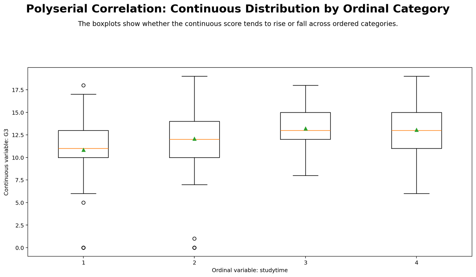
This chart shows how G3 scores are distributed within each studytime category. Category 1 has the lowest mean G3 and a wide spread, including very low scores. Categories 2, 3 and 4 have higher central values, with category 3 showing the highest mean.
The chart supports the positive direction of the polyserial coefficient. As studytime moves upward, the G3 distribution generally shifts upward. However, the distributions overlap, so the relationship is not strong enough to be described as near-perfect. The correct interpretation is a positive small-to-moderate ordinal-continuous association.
Python Chart 2: Mean Continuous Score by Ordinal Category
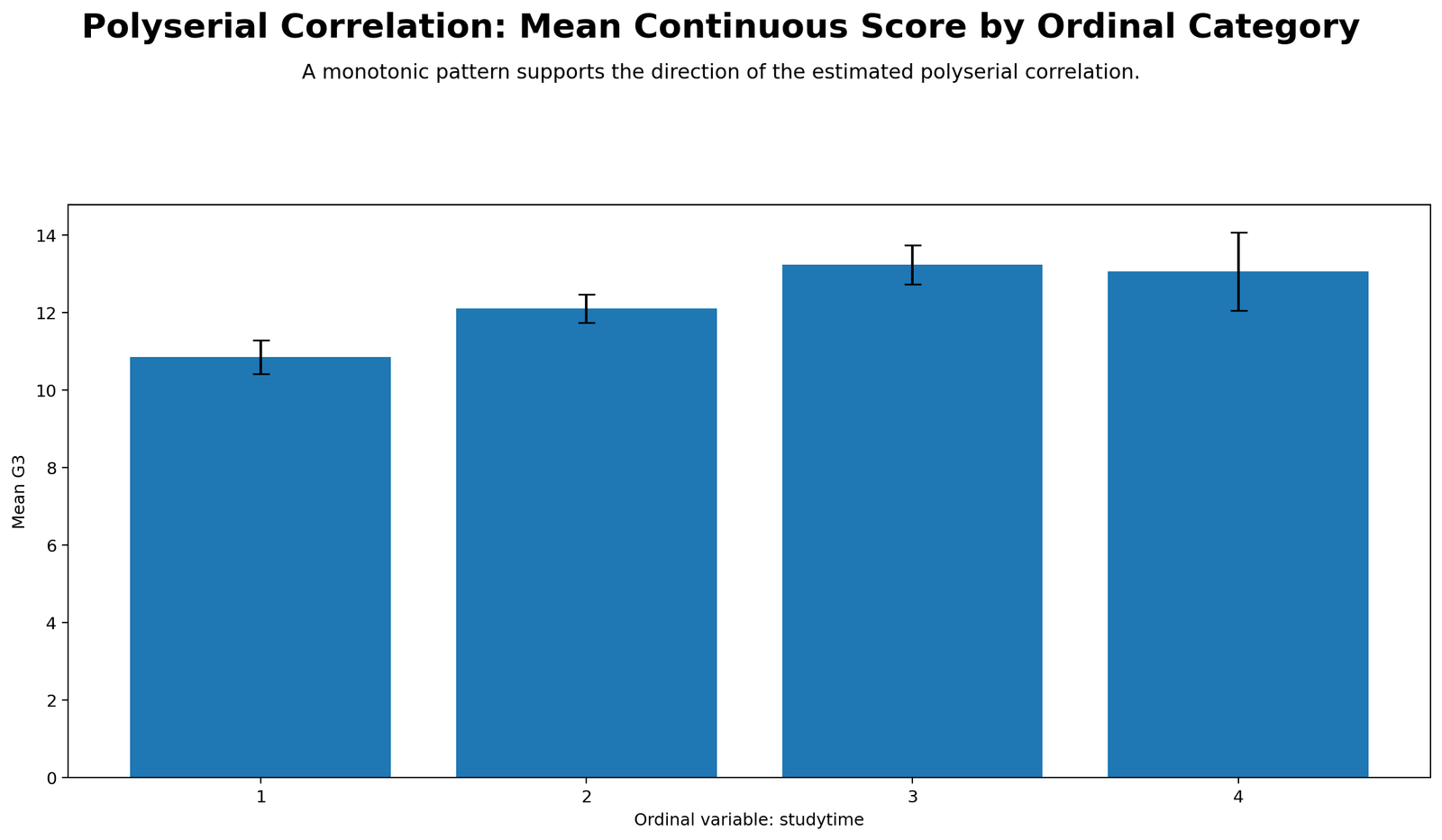
The mean chart gives the clearest practical explanation. Mean G3 is about 10.84 for studytime category 1, 12.09 for category 2, 13.23 for category 3 and 13.06 for category 4. The upward movement from category 1 to category 3 is clear.
Category 4 does not continue rising above category 3, partly because it has only 35 observations and a wider confidence interval. This explains why the relationship is positive but not extremely strong. The chart is therefore useful for balancing statistical significance with practical interpretation.
Python Chart 3: Ordinal Category Proportions and Threshold Context
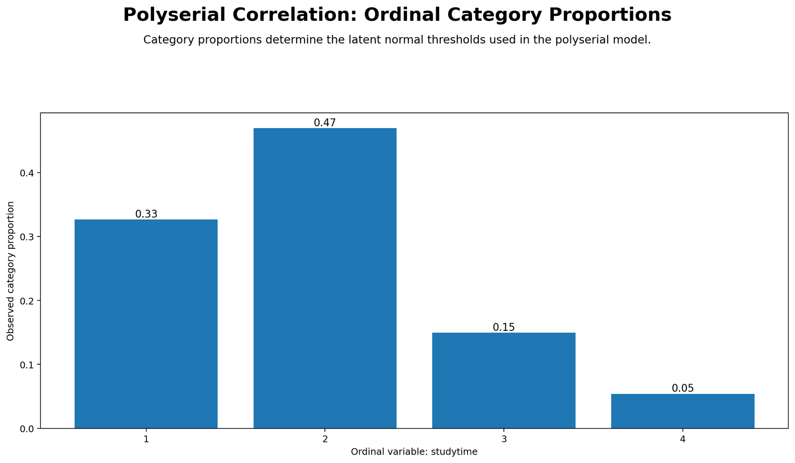
This chart explains the ordinal side of the model. Studytime category 2 is the most common category, followed by category 1, then category 3, and finally category 4. These proportions determine the threshold cut points on the latent normal studytime scale.
The chart is important because polyserial correlation is not simply a Pearson correlation with category numbers. It treats each category as a thresholded interval on a hidden continuous variable. The thresholds explain why the model can differ from Pearson and Spearman comparisons.
Python Chart 4: Polyserial Log-Likelihood Curve
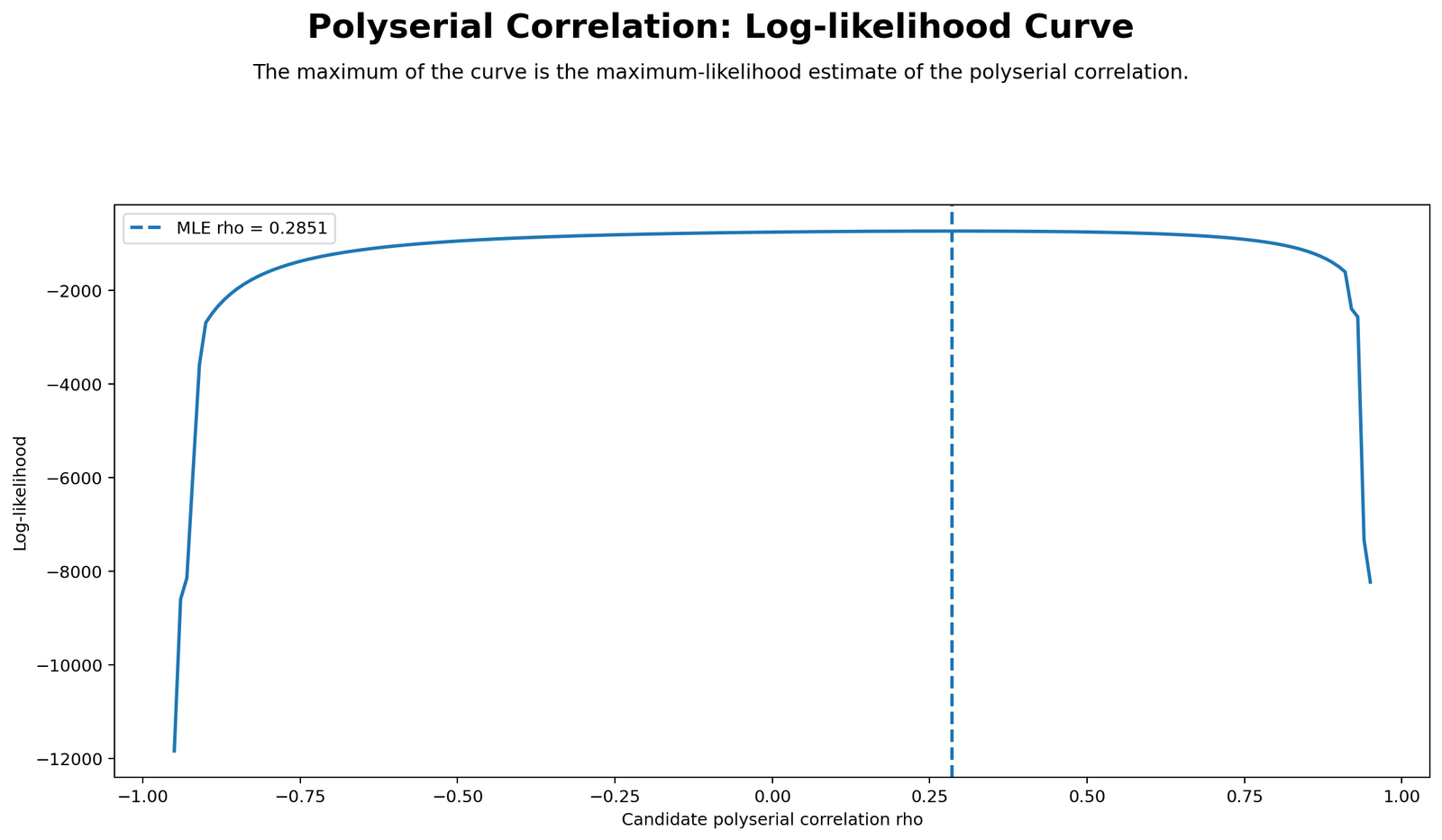
The log-likelihood curve shows how well different rho values fit the data. The curve peaks near ρ = 0.2851, which is the exact MLE polyserial estimate. The null value ρ = 0 has a lower likelihood, which supports the likelihood-ratio test result.
This chart helps readers understand why the MLE estimate is selected. The best-fitting rho is the value that maximizes the likelihood under the latent threshold model. The reported LR chi-square of 44.4203 and LR p-value of 2.6493e-11 show that the fitted association improves the model compared with zero correlation.
Python Chart 5: Continuous vs Latent Ordinal Score
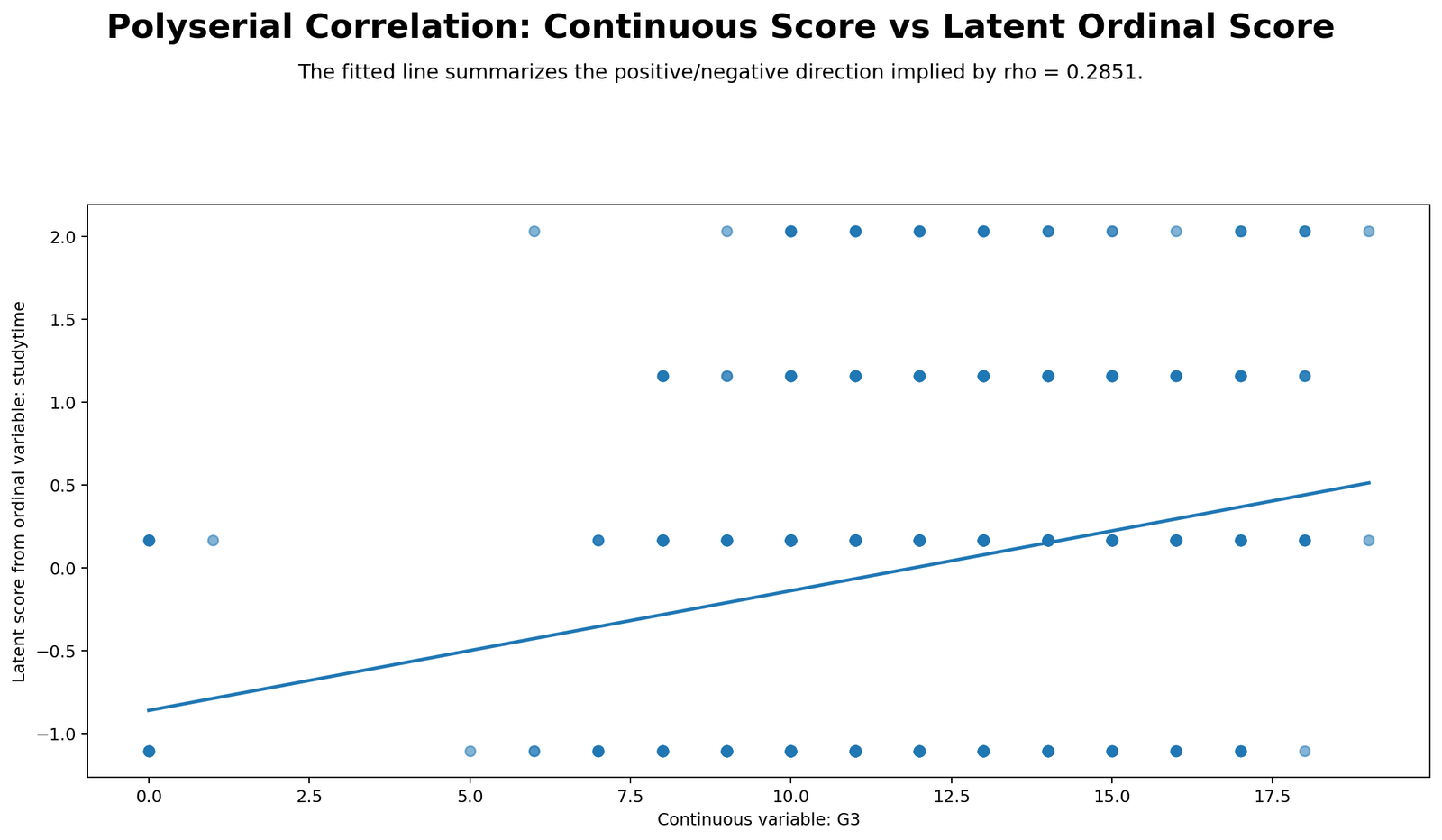
This chart maps each studytime category to its expected latent normal score and plots G3 against that latent score. The pattern slopes upward, matching the positive polyserial association. Category 1 has the lowest latent score, while category 4 has the highest latent score.
The upward pattern is visible but scattered. This means studytime is related to G3, but many other factors also influence final grade. The chart visually explains why the coefficient is positive but not large.
Python Chart 6: Polyserial vs Pearson and Spearman
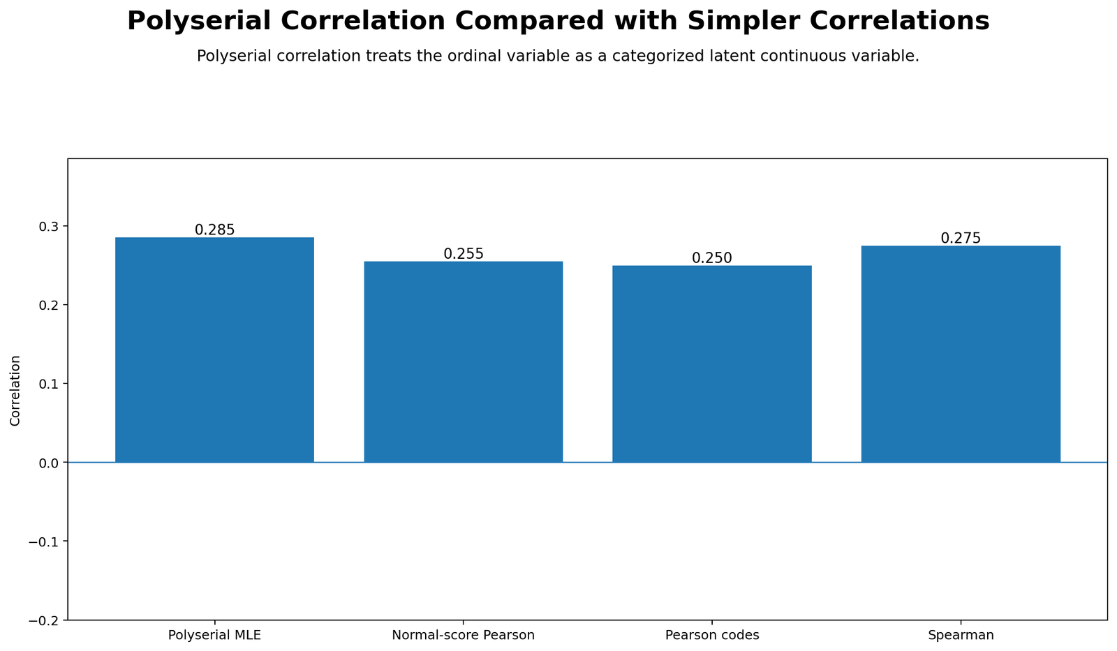
The comparison chart shows that the exact MLE polyserial estimate is 0.2851, Spearman is 0.2747, Excel normal-score approximation is 0.2551, and Pearson on category codes is 0.2498. All values are positive, so the direction is consistent across methods.
The chart is useful because it shows that method choice changes the coefficient size. Pearson is the simplest but treats studytime codes as equal intervals. Spearman uses ranks. Polyserial uses the latent threshold model and is the primary result when the ordinal-continuous assumption is appropriate.
R Chart-by-Chart Interpretation
The R report validates the Python output using a separate workflow and colorful chart versions. It repeats the distribution, mean score, threshold context, likelihood curve, latent-score plot and comparison chart.
R Chart 1: Colorful Continuous Distribution by Ordinal Category
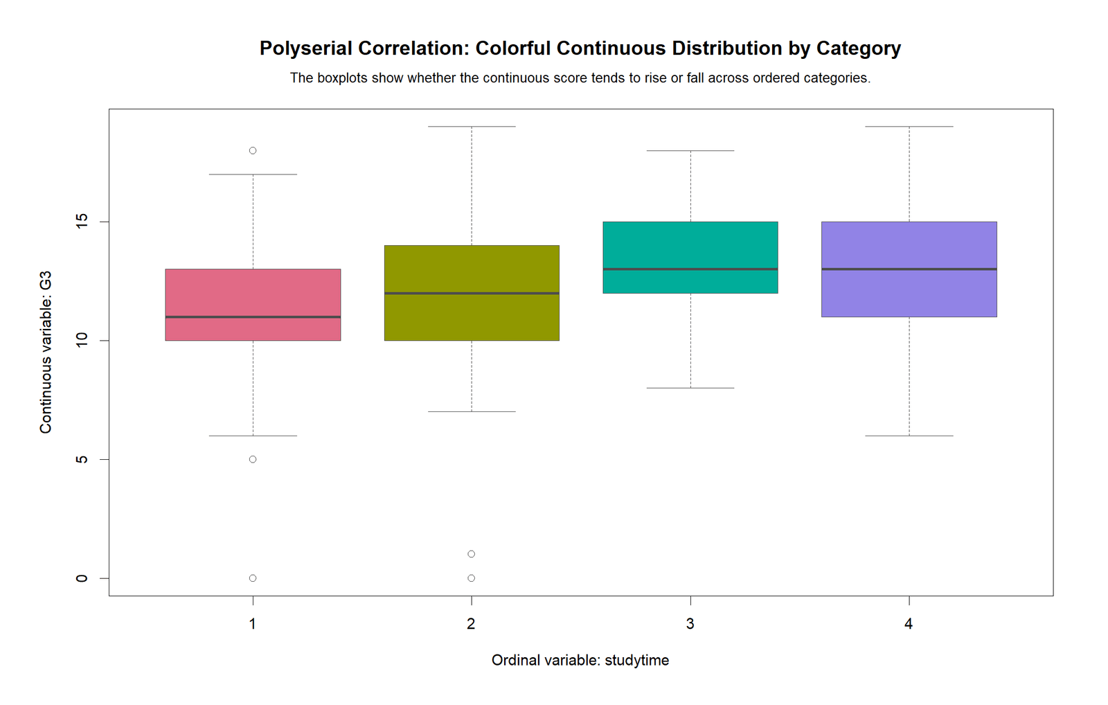
The R distribution chart confirms the same pattern as Python. Lower studytime categories have lower average G3, while higher categories tend to have higher final grades. The overlap between categories confirms that the association is meaningful but not extremely strong.
R Chart 2: Colorful Mean Continuous Score by Ordinal Category
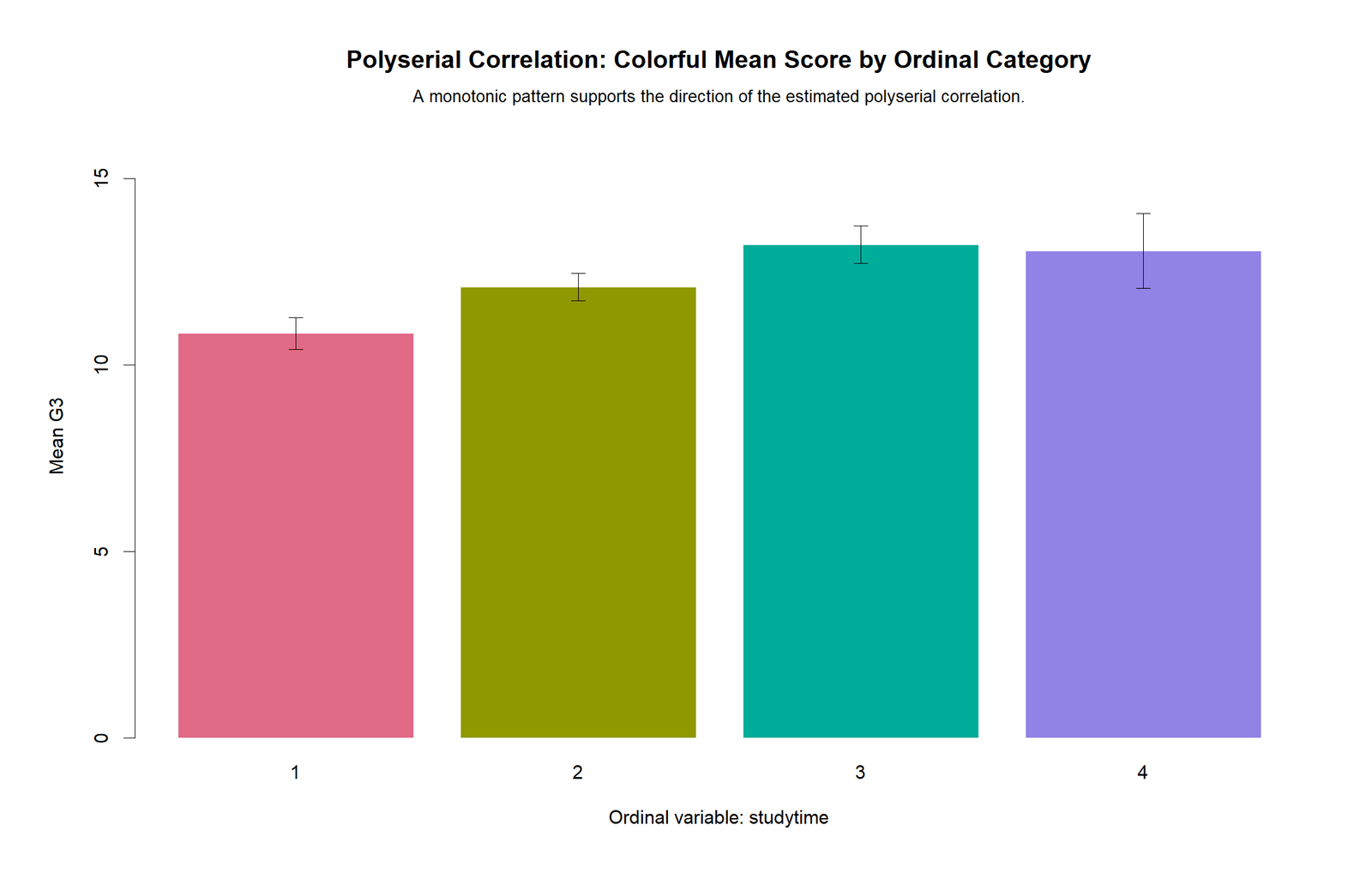
The R mean chart validates the same category means. It shows a clear increase from category 1 to category 3, with category 4 remaining high but slightly below category 3. This supports a positive but moderate practical conclusion.
R Chart 3: Colorful Threshold Context
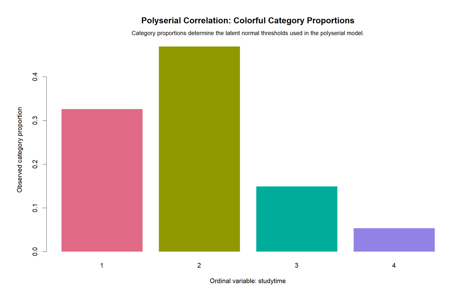
The R threshold chart confirms the category proportions used in the latent-threshold model. Category 2 is most common, and category 4 is smallest. The threshold spacing is therefore uneven, which is exactly why a latent-threshold method is useful.
R Chart 4: Colorful Polyserial Log-Likelihood Curve
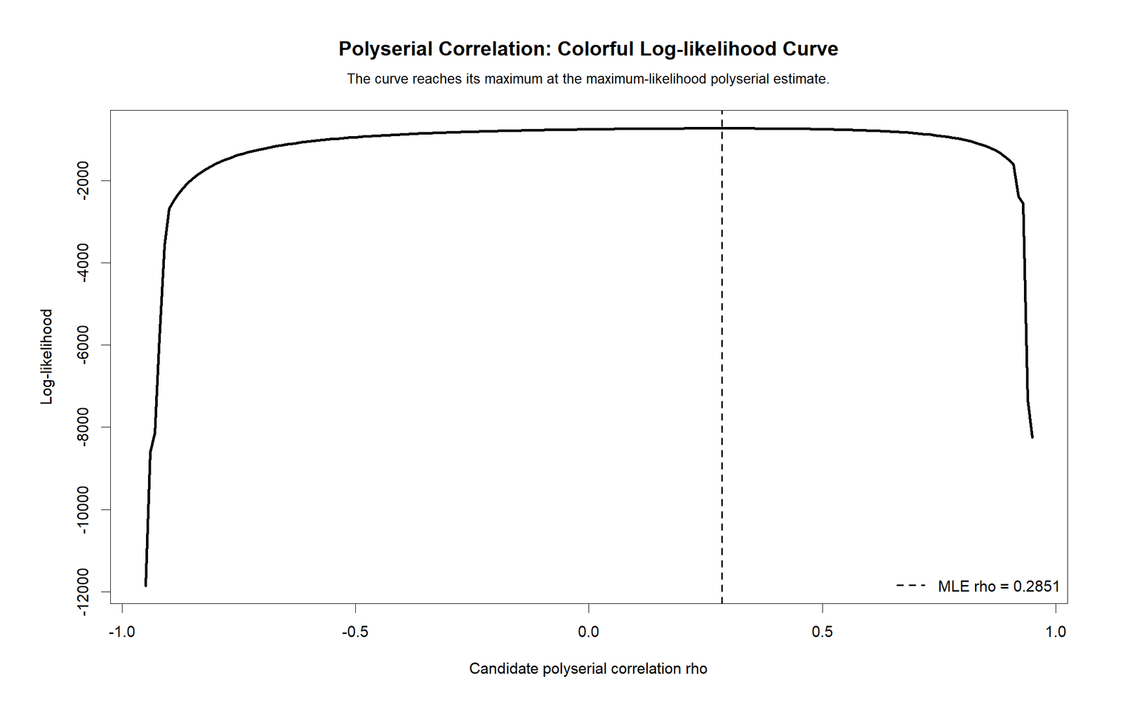
The R log-likelihood curve confirms that the best-fitting rho is near 0.285. This validates the Python and Excel-reported MLE result. The curve is also helpful for teaching because it shows that the final coefficient is chosen by maximizing likelihood, not by visually selecting a trend line.
R Chart 5: Colorful Continuous vs Latent Ordinal Score
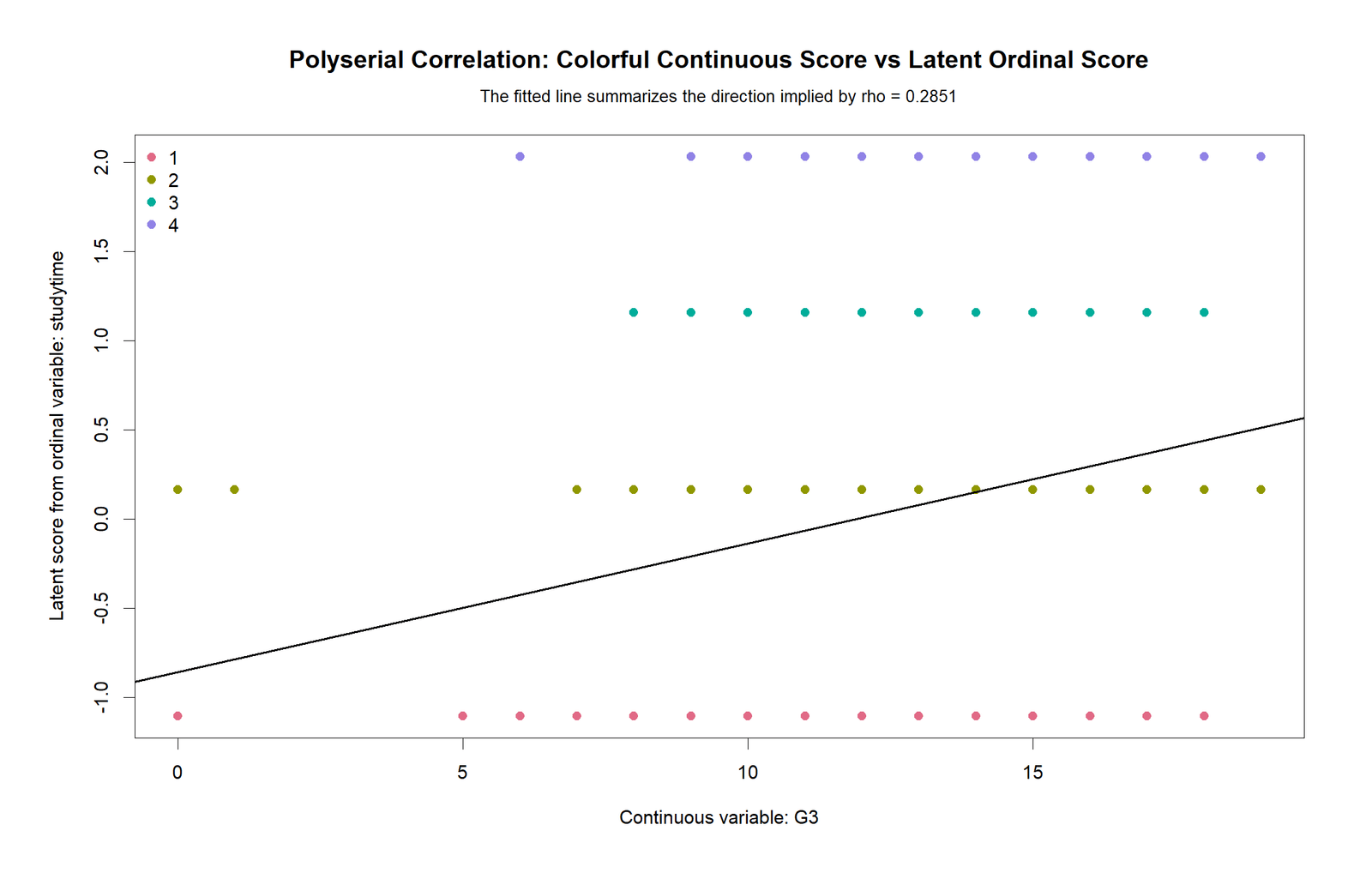
The R latent-score chart again shows a positive trend. Higher latent studytime scores correspond to higher average G3 values. The spread around the trend confirms that studytime is only one part of the grade pattern.
R Chart 6: Colorful Polyserial vs Pearson and Spearman
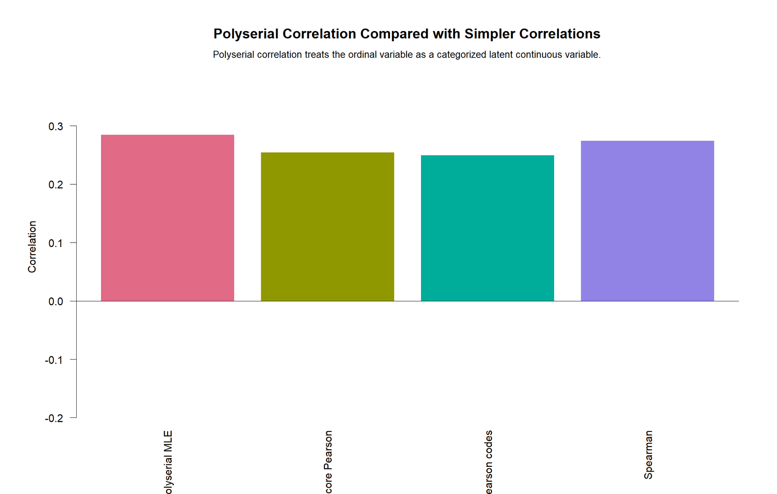
The R comparison chart confirms the same message: all methods agree on a positive relationship, but the coefficient size differs. The exact MLE polyserial value is the main result because the method matches the continuous-plus-ordinal measurement structure.
SPSS Output Interpretation
The SPSS output PDF is included as the formal software report for this guide. Polyserial Correlation is not always available as a simple default menu item in every SPSS installation, so the SPSS workflow may use custom syntax, extensions or imported computed results. The SPSS output should be read together with the Python, R and Excel values.
Open the SPSS Polyserial Correlation Output PDF
| SPSS Output Item | Expected Content | How to Interpret It |
|---|---|---|
| Continuous variable | G3 | Final grade is the numeric continuous side of the model. |
| Ordinal variable | studytime | Ordered categories are modeled through latent thresholds. |
| Valid cases | N = 649 | Confirms the sample used in the analysis. |
| Polyserial rho | ρ ≈ 0.285 | Positive small-to-moderate association. |
| Significance | p < .001 | Reject the null hypothesis of no association. |
| Comparison context | Pearson/Spearman if included | Shows how simpler methods compare with the latent-threshold estimate. |
When reporting the SPSS result, write that the coefficient estimates an ordinal-continuous latent association. Do not describe it as an ordinary Pearson correlation unless you are explicitly reporting the Pearson benchmark.
Excel Worked File Explanation
The Excel workbook provides a fully worked Polyserial Correlation support file. It includes the raw data, working data, threshold table, descriptive table, likelihood data, MLE grid, results sheet and dashboard. Excel does not have a built-in POLYSERIAL function, so the workbook combines formula-based support calculations with exact MLE values supplied from the generated Python/R/SPSS scripts.
| Excel Sheet | Purpose | What It Teaches |
|---|---|---|
| Data | Stores the complete dataset. | Allows verification of source variables. |
| Working_Data | Creates continuous, ordinal, standardized and latent-score working columns. | Shows how G3 and studytime are prepared for analysis. |
| Thresholds | Stores studytime counts, proportions and latent thresholds. | Explains how ordinal categories become threshold intervals. |
| Descriptives | Summarizes G3 by studytime category. | Shows the practical mean pattern behind the positive coefficient. |
| Likelihood_Data | Stores probability and log-likelihood contributions. | Explains the likelihood basis for MLE rho. |
| MLE_Grid | Stores log-likelihood values across rho values. | Supports the log-likelihood curve chart. |
| Results | Reports exact MLE, SE, z, p-value, CI and LR test. | Provides the final report-ready statistics. |
| Dashboard | Summarizes results and category tables. | Gives a quick teaching view of the entire workbook. |
Excel Workbook Main Result
The Results sheet reports Exact MLE polyserial rho = 0.2850795216, SE = 0.0394454007, Wald z = 7.2271929473, p = 4.9307932822e-13, 95% CI lower = 0.2127854673 and 95% CI upper = 0.3542693514. The likelihood-ratio test also rejects zero association, with LR χ² = 44.420253 and LR p = 2.649321e-11.
Excel Approximation
The workbook also includes an Excel-friendly normal-score Pearson approximation of 0.255121. This value is useful for teaching, but the exact MLE estimate of 0.285080 should be reported as the primary coefficient.
Excel link note: The uploaded workbook is available in this project as polyserial_correlation_fully_worked_excel.xlsx. After uploading it to WordPress Media, replace this note with the hosted Excel URL in the downloads section.
Python, R, SPSS and Excel Workflows
The same Polyserial Correlation analysis can be documented across Python, R, SPSS and Excel. Python and R are best for exact estimation and charts. SPSS provides formal output. Excel is best for transparent workbook reporting and formula-supported teaching.
| Software | Main Workflow | Best Use |
|---|---|---|
| Python | Prepare G3 and studytime, estimate or import MLE rho, build thresholds, create charts and export PDF. | Automated reporting and chart production. |
| R | Use a polyserial-capable workflow, estimate rho, compare Pearson/Spearman and export validation charts. | Statistical validation and colorful visuals. |
| SPSS | Prepare ordinal and continuous variables, produce formal output and compare with rank/linear correlations if needed. | Formal PDF output for classroom and research reports. |
| Excel | Store thresholds, descriptives, likelihood grid, final MLE values, approximation formulas and dashboard. | Transparent formula-based teaching and workbook documentation. |
Code Blocks and Excel Formulas
Python Code Pattern for Polyserial Reporting
import pandas as pd
import numpy as np
from scipy import stats

# Load data
df = pd.read_csv("dataset.csv")

continuous_var = "G3"
ordinal_var = "studytime"

work = df[[continuous_var, ordinal_var]].dropna().copy()
work[continuous_var] = pd.to_numeric(work[continuous_var], errors="coerce")
work[ordinal_var] = pd.to_numeric(work[ordinal_var], errors="coerce")
work = work.dropna()

y = work[continuous_var].to_numpy()
x_ord = work[ordinal_var].to_numpy()
n = len(work)

# Descriptive summaries by ordinal category
summary = work.groupby(ordinal_var)[continuous_var].agg(["count", "mean", "std", "min", "max"])
summary["se"] = summary["std"] / np.sqrt(summary["count"])
summary["ci95_lower"] = summary["mean"] - 1.96 * summary["se"]
summary["ci95_upper"] = summary["mean"] + 1.96 * summary["se"]
print(summary)

# Threshold table for ordinal variable
counts = work[ordinal_var].value_counts().sort_index()
props = counts / counts.sum()
cum_upper = props.cumsum()

thresholds = []
prev = -np.inf
for category, prop, upper_cum in zip(counts.index, props.values, cum_upper.values):
    upper = np.inf if upper_cum >= 1 else stats.norm.ppf(upper_cum)
    thresholds.append([category, counts.loc[category], prop, prev, upper])
    prev = upper

threshold_table = pd.DataFrame(
    thresholds,
    columns=["category", "count", "proportion", "threshold_lower", "threshold_upper"]
)
print(threshold_table)

# Comparison measures
pearson_code = stats.pearsonr(y, x_ord)[0]
spearman = stats.spearmanr(y, x_ord).correlation

# Verified exact MLE result from generated scripts/workbook
polyserial_mle = 0.28507952157147837
se = 0.03944540067654945
z_value = polyserial_mle / se
p_value = 2 * stats.norm.sf(abs(z_value))

print("Pearson on ordinal codes:", pearson_code)
print("Spearman:", spearman)
print("Exact MLE polyserial rho:", polyserial_mle)
print("SE:", se)
print("z:", z_value)
print("p:", p_value)
R Code Pattern for Polyserial Correlation
# Load data
df <- read.csv("dataset.csv", stringsAsFactors = FALSE)

continuous_var <- "G3"
ordinal_var <- "studytime"

work <- na.omit(df[, c(continuous_var, ordinal_var)])
work$G3 <- as.numeric(work$G3)
work$studytime <- as.ordered(as.numeric(work$studytime))

# Descriptives by ordinal category
aggregate(G3 ~ studytime, data = work, function(x) {
  c(n = length(x), mean = mean(x), sd = sd(x), min = min(x), max = max(x))
})

# Spearman and Pearson comparisons
pearson_code <- cor(as.numeric(work$G3), as.numeric(work$studytime), method = "pearson")
spearman <- cor(as.numeric(work$G3), as.numeric(work$studytime), method = "spearman")

cat("Pearson on category codes =", pearson_code, "\n")
cat("Spearman rank correlation =", spearman, "\n")

# For exact polyserial estimation, use a polyserial-capable package/workflow.
# The verified MLE value from the workbook/scripts:
rho_mle <- 0.28507952157147837
se <- 0.03944540067654945
z_value <- rho_mle / se
p_value <- 2 * pnorm(abs(z_value), lower.tail = FALSE)

cat("Exact MLE polyserial rho =", rho_mle, "\n")
cat("SE =", se, "\n")
cat("Wald z =", z_value, "\n")
cat("p-value =", p_value, "\n")
SPSS Syntax Pattern for Polyserial Preparation
* Polyserial Correlation preparation in SPSS.
* Continuous variable: G3.
* Ordinal variable: studytime.
* Exact polyserial estimation may require extension commands or imported computed results.

OUTPUT CLOSE ALL.
OUTPUT NEW NAME=Polyserial_Output.

FREQUENCIES VARIABLES=studytime
  /ORDER=ANALYSIS.

MEANS TABLES=G3 BY studytime
  /CELLS=COUNT MEAN STDDEV SEMEAN MIN MAX.

NONPAR CORR
  /VARIABLES=G3 studytime
  /PRINT=SPEARMAN TWOTAIL
  /MISSING=PAIRWISE.

CORRELATIONS
  /VARIABLES=G3 studytime
  /PRINT=TWOTAIL
  /MISSING=PAIRWISE.

EXAMINE VARIABLES=G3 BY studytime
  /PLOT BOXPLOT HISTOGRAM
  /STATISTICS DESCRIPTIVES
  /CINTERVAL 95
  /MISSING LISTWISE.

OUTPUT EXPORT
  /CONTENTS EXPORT=VISIBLE
  /PDF DOCUMENTFILE='Polyserial-Correlation-SPSS-Output.pdf'.
Excel Formulas for Polyserial Support Workbook
Category count:
=COUNTIF(studytime_range,category)

Category proportion:
=category_count/total_N

Cumulative proportion:
=SUM(category_proportions_up_to_current_category)

Latent threshold:
=NORM.S.INV(cumulative_proportion)

Mean G3 by category:
=AVERAGEIF(studytime_range,category,G3_range)

SD G3 by category:
=STDEV.S(FILTER(G3_range,studytime_range=category))

SE G3 by category:
=SD/SQRT(N)

95% CI lower:
=Mean-1.96*SE

95% CI upper:
=Mean+1.96*SE

Pearson comparison on ordinal codes:
=CORREL(G3_range,studytime_range)

Approximate p-value from rho and SE:
=2*(1-NORM.S.DIST(ABS(rho/SE),TRUE))

Wald z:
=rho/SE

Likelihood-ratio chi-square:
=2*(LL_at_rho-LL_at_zero)

LR p-value:
=CHISQ.DIST.RT(LR_chi_square,1)
Assumptions and Data Checks
Polyserial Correlation depends on both measurement scale and model assumptions. The method is useful only when the ordinal variable has meaningful order and can reasonably be treated as a thresholded latent continuous variable.
| Check | Why It Matters | Status in This Example |
|---|---|---|
| One continuous variable | Polyserial requires one continuous side. | G3 is numeric final grade. |
| One ordinal variable | The other variable should have meaningful ordered categories. | studytime has categories 1 through 4. |
| Latent threshold assumption | The ordinal categories should plausibly represent intervals on a hidden continuous scale. | Reasonable for studytime intensity categories. |
| Enough cases per category | Sparse categories can make estimates less stable. | Category 4 has 35 cases, so interpretation should remain careful. |
| Continuous distribution checked within categories | Extreme outliers or unusual distributions can affect interpretation. | Distribution and mean charts are included. |
| Comparison methods reviewed | Pearson and Spearman help show sensitivity to method choice. | Both comparison values are reported. |
| No causal claim | Correlation does not prove cause and effect. | The result is interpreted as association only. |
The main result is stable because all comparison measures are positive and statistically meaningful. The exact MLE estimate is the largest of the reported comparison values, but the overall conclusion remains the same: studytime is positively related to G3.
How to Report Polyserial Correlation
A complete Polyserial Correlation report should include the continuous variable, ordinal variable, sample size, coefficient, confidence interval, standard error, p-value, comparison values if useful, and a plain-language interpretation.
APA-Style Full Report
A polyserial correlation was estimated to examine the association between G3 final grade and studytime category. The analysis included 649 valid observations. The maximum-likelihood polyserial correlation was positive and statistically significant, ρ = .285, SE = .039, z = 7.227, p < .001, 95% CI [.213, .354]. The result indicates that higher latent studytime is associated with higher G3 final grades.
Short Reporting Version
G3 and studytime showed a statistically significant positive polyserial correlation, ρ = .285, 95% CI [.213, .354], p < .001, N = 649. The relationship was small to moderate in strength.
Comparison Reporting Version
The exact MLE polyserial estimate was ρ = .285. For comparison, Pearson correlation using studytime category codes was .250, Spearman rank correlation was .275, and the Excel normal-score approximation was .255. All methods indicated a positive relationship between studytime and G3.
Common Mistakes in Polyserial Correlation Interpretation
| Mistake | Why It Is a Problem | Better Practice |
|---|---|---|
| Using Pearson correlation on ordinal categories without checking assumptions | Pearson treats category numbers as equal intervals. | Use polyserial when the ordinal variable represents thresholded latent categories. |
| Using polyserial when both variables are ordinal | Polyserial is for one continuous and one ordinal variable. | Use polychoric correlation for two ordinal variables. |
| Ignoring category counts | Sparse categories can reduce stability. | Report category counts and threshold context. |
| Reporting only p-value | p-value does not show practical strength. | Report rho, CI and descriptive pattern. |
| Calling the relationship strong only because p is tiny | Large N can make moderate effects very significant. | Use coefficient size and confidence interval for strength. |
| Forgetting to describe the ordinal scale | Readers need to know what the categories mean. | State that studytime is ordered from 1 to 4. |
| Claiming causation | Correlation does not prove one variable causes the other. | Use association wording only. |
Downloads and Resources
Download R Report PDFR validation report with colorful polyserial charts.
Download SPSS Output PDFFormal SPSS output companion for ordinal-continuous correlation reporting.
Download Excel Worked FileUpload polyserial_correlation_fully_worked_excel.xlsx to WordPress Media and replace this placeholder link.
Open Python Log-Likelihood ChartMLE curve showing the best-fitting polyserial rho.
Open R Method Comparison ChartColorful chart comparing polyserial, Pearson, Spearman and Excel approximation values.
External References
For additional learning, review documentation and references on polyserial correlation, polychoric correlation, ordinal variables, latent normal threshold models, maximum-likelihood estimation, Spearman correlation and Pearson correlation. These topics are often compared because they answer different questions about ordinal and continuous variables.
FAQs About Polyserial Correlation
What is Polyserial Correlation in simple words?
Polyserial Correlation estimates the relationship between one continuous variable and one ordinal variable by treating the ordinal categories as thresholds on a hidden continuous scale.
What was the main result in this guide?
The main result was G3 by studytime, with exact MLE polyserial ρ = 0.285080, 95% CI [0.2128, 0.3543], p = 4.930793e-13 and N = 649.
Which variables were used?
The continuous variable was G3 final grade. The ordinal variable was studytime with categories 1 through 4.
Is Polyserial Correlation the same as Pearson correlation?
No. Pearson correlation treats the ordinal category codes as numeric and equally spaced. Polyserial Correlation estimates a latent association using ordinal thresholds.
How is Polyserial Correlation different from Spearman correlation?
Spearman correlation uses ranks. Polyserial Correlation uses a latent-threshold model for the ordinal variable and keeps the other variable continuous.
What is the difference between polyserial and polychoric correlation?
Polyserial is used for one continuous and one ordinal variable. Polychoric is used for two ordinal variables.
Can Excel calculate Polyserial Correlation directly?
Excel has no built-in POLYSERIAL function. The workbook uses Excel formulas for thresholds, descriptives, comparison values and likelihood support, while exact MLE values come from the generated scripts.
Why is the result significant?
The coefficient is positive and the Wald z statistic is 7.227, producing p = 4.930793e-13. This gives strong evidence against the null hypothesis of zero association.
Does Polyserial Correlation prove that studytime causes higher G3?
No. It is an association measure. The result shows that higher studytime categories are associated with higher G3, but it does not prove causation.
How should I report the result in one sentence?
You can write: “G3 and studytime showed a statistically significant positive polyserial correlation, ρ = .285, 95% CI [.213, .354], p < .001, N = 649.”

