
Binary-continuous correlation, group mean difference, t-test connection and Excel worked result
Point Biserial Correlation: Formula, Interpretation, SPSS, Python, R and Excel Guide
Point Biserial Correlation measures the association between one true binary variable and one continuous variable. It is mathematically the same as Pearson correlation when the binary variable is coded 0 and 1, but its interpretation focuses on the difference between two group means. This guide explains the formula, assumptions, binary coding, group mean interpretation, Python charts, R validation charts, SPSS output, Excel formulas, p-value, t-test connection, APA reporting, common mistakes and downloadable files.
Quick Answer: Point Biserial Correlation Result
The main worked example tests the association between sex and G3 final grade. The binary variable is sex, coded as F = 0 and M = 1. The continuous variable is G3. Since sex is a true two-category variable and G3 is a numeric grade score, the correct correlation is Point Biserial Correlation.
The verified Excel result is rpb = -0.129077, with N = 649, t(647) = -3.310938, and p = 0.000982. The result is statistically significant at α = .05, but the effect size is small. The negative sign appears because the group coded 1, which is M, has a lower mean G3 score than the group coded 0, which is F.
Final interpretation: There is a statistically significant small negative point-biserial association between sex coding and G3 final grade. Because M was coded as 1 and had a lower mean G3 score than F, the coefficient is negative. The relationship is statistically detectable, but the practical strength is small.
Important reporting point: Do not report only the p-value. The p-value is significant, but rpb = -0.129 is small and r² = 0.0167, meaning the binary coding explains only about 1.67% of the variance in G3.
Table of Contents
- What Is Point Biserial Correlation?
- When Should You Use Point Biserial Correlation?
- Point Biserial vs Biserial vs Phi Coefficient
- Point Biserial Correlation Formula
- Null and Alternative Hypotheses
- Dataset and Variables Used
- Verified Point Biserial Results
- Top Pairwise Point Biserial Relationships
- Python Chart-by-Chart Interpretation
- R Chart-by-Chart Interpretation
- SPSS Output Interpretation
- Excel Worked File Explanation
- Python, R, SPSS and Excel Workflows
- Code Blocks and Excel Formulas
- Assumptions and Data Checks
- How to Report Point Biserial Correlation
- Common Mistakes
- Downloads and Resources
- Related Statistical Guides
- FAQs About Point Biserial Correlation
What Is Point Biserial Correlation?
Point Biserial Correlation is a correlation coefficient used when one variable is naturally binary and the other variable is continuous. A binary variable has two categories, such as female/male, yes/no, pass/fail, treatment/control, urban/rural, public/private, or present/absent. A continuous variable has numeric values, such as final grade, test score, income, weight, time, age, or measurement score.
The point-biserial coefficient is written as rpb. It is calculated like Pearson correlation after the binary variable is coded as 0 and 1. Even though the calculation is correlation-based, the interpretation is often easier through group means. A positive rpb means the group coded 1 has a higher mean on the continuous variable. A negative rpb means the group coded 1 has a lower mean.
In this guide, F is coded 0 and M is coded 1. The F group has mean G3 = 12.2533, while the M group has mean G3 = 11.4060. Since the group coded 1 has the lower mean, the point-biserial correlation is negative: rpb = -0.129077.
Point Biserial Correlation connects naturally with Correlation in Python, Correlation in R, Correlation in SPSS, Correlation in Excel, t-Test in Python, t-Test in SPSS, Effect Size, p-value and Confidence Interval.
Simple definition: Point Biserial Correlation measures the relationship between a true 0/1 binary variable and a continuous variable. It is Pearson correlation with one variable coded 0 and 1.
When Should You Use Point Biserial Correlation?
Use Point Biserial Correlation when the research question asks whether a two-category group variable is associated with a numeric outcome. The binary variable should be a real two-category variable, not an artificial split made from a continuous variable. The continuous variable should have meaningful numeric distances.
| Situation | Use Point Biserial? | Reason | Example |
|---|---|---|---|
| One true binary variable and one continuous variable | Yes | This is the standard use case. | sex coded 0/1 with G3 final grade. |
| Binary group is naturally two categories | Yes | Point-biserial is for true dichotomies. | school GP/MS with G1 score. |
| Binary variable is yes/no and outcome is a score | Yes | 0/1 coding can be correlated with the score. | higher education yes/no with G3 score. |
| Both variables are binary | No | Use Phi Coefficient or chi-square for a 2×2 table. | sex by pass/fail status. |
| Binary variable is an artificial split of a continuous variable | Usually not the best name | Biserial correlation may be discussed if the split represents an underlying continuous trait. | G1 converted to low/high by cutoff. |
| Both variables are continuous | No | Use Pearson, Spearman, Kendall Tau-b, or another continuous/rank method. | G1 and G3 as numeric grades. |
For the main worked example, the conditions are satisfied. Sex is binary, G3 is continuous/numeric, and the analysis asks whether the binary group coding is associated with final grade. The result is statistically significant, but the group mean difference is modest and the effect size is small.
Point Biserial vs Biserial vs Phi Coefficient
Students often mix up Point Biserial Correlation, Biserial Correlation, and Phi Coefficient because all three involve binary variables. The key difference is the scale of the second variable and whether the binary variable is a true binary variable or an artificial split.
| Measure | Use It When | Example | Main Interpretation |
|---|---|---|---|
| Point Biserial Correlation | One variable is truly binary and the other is continuous. | sex coded F=0, M=1 with G3 score. | Observed correlation between binary coding and continuous score. |
| Biserial Correlation | The binary variable is an artificial split from an underlying continuous trait. | G1 split into low/high using a cutoff. | Estimated association before the artificial split. |
| Phi Coefficient | Both variables are binary. | sex by pass/fail status. | Association in a 2×2 contingency table. |
| Independent Samples t-Test | One binary group variable and one continuous outcome. | Compare mean G3 for F and M. | Tests whether the two group means differ. |
Reporting rule: If your binary variable is real and your outcome is continuous, report Point Biserial Correlation. If both variables are binary, report Phi Coefficient. If the binary variable is created by splitting a continuous trait, discuss Biserial Correlation carefully.
Point Biserial Correlation Formula
Point Biserial Correlation can be calculated using Pearson correlation after coding the binary variable as 0 and 1. It can also be calculated from group means, sample standard deviation, and group sizes.
In this formula, M1 is the mean of the continuous variable for the group coded 1, M0 is the mean for the group coded 0, SDY is the sample standard deviation of the continuous variable, n1 and n0 are the group sizes, and n is the total sample size.
| Formula Element | Meaning | Verified Value |
|---|---|---|
| M0 | Mean G3 for F coded 0 | 12.2532637076 |
| M1 | Mean G3 for M coded 1 | 11.4060150376 |
| M1 − M0 | Mean difference for code 1 minus code 0 | -0.8472486700 |
| SDY | Sample standard deviation of G3 | 3.2306562428 |
| n0 | F group size | 383 |
| n1 | M group size | 266 |
| n | Total valid observations | 649 |
| rpb | Point Biserial Correlation | -0.1290774866 |
The sign is negative because the group coded 1 has a lower mean. If the coding were reversed, the sign would change, but the absolute strength would remain the same.
Significance Test Formula
The point-biserial significance test can be written using the same t-test logic used for Pearson correlation:
For the main example, this gives t = -3.310938, with df = 647 and p = 0.000982. The r-squared value is 0.016661, so the binary coding accounts for about 1.67% of the variance in G3.
Null and Alternative Hypotheses
The point-biserial test asks whether the population association between the binary variable and the continuous variable is zero.
| Statement | Hypothesis | Meaning |
|---|---|---|
| Null hypothesis | H0: ρpb = 0 | There is no association between sex coding and G3 final grade in the population. |
| Alternative hypothesis | H1: ρpb ≠ 0 | There is an association between sex coding and G3 final grade. |
| Observed direction | rpb < 0 | The group coded 1 has a lower mean G3 score than the group coded 0. |
| Decision rule | Reject H0 if p < .05 | The association is statistically significant at the 5% level. |
Decision: Since p = 0.000982 is below .05, the null hypothesis is rejected. There is a statistically significant association between sex coding and G3. The effect size is small because rpb = -0.129077.
Dataset and Variables Used
The analysis uses the student performance dataset with 649 valid observations. The main worked example uses sex as the true binary variable and G3 as the continuous outcome variable.
| Variable | Role | Coding / Scale | Purpose in This Test |
|---|---|---|---|
| sex | Binary predictor | F = 0, M = 1 | Defines the two groups compared by point-biserial correlation. |
| G3 | Continuous outcome | Final grade score, observed 0 to 19 | Numeric variable being compared across the two binary groups. |
| G1 and G2 | Additional continuous outcomes | First and second period grades | Used in pairwise point-biserial screening with binary variables. |
| higher | Additional binary predictor | no = 0, yes = 1 | Strongest pairwise point-biserial relationship with G1 in the workbook. |
| school, address, internet | Additional binary predictors | Two-category variables | Used for broader binary-continuous association screening. |
Before reporting the coefficient, it is useful to review Descriptive Statistics Explained, Standard Deviation, Standard Error, Confidence Interval, Effect Size, p-value and Null and Alternative Hypothesis.
Verified Point Biserial Results
The table below summarizes the verified main worked example from the Excel workbook. The values match the report-card logic used in the Python and R charts.
| Statistic | Verified Value | Interpretation |
|---|---|---|
| Continuous variable | G3 | Final grade score. |
| Binary variable | sex | True binary grouping variable. |
| Coding | F = 0, M = 1 | The sign depends on this coding. |
| N | 649 | Complete valid observations. |
| n code 0 | 383 | F group size. |
| n code 1 | 266 | M group size. |
| Proportion code 0 | 0.590139 | F group proportion. |
| Proportion code 1 | 0.409861 | M group proportion. |
| Mean G3 for code 0 | 12.253264 | F group mean. |
| Mean G3 for code 1 | 11.406015 | M group mean. |
| Mean difference 1 − 0 | -0.847249 | M mean is lower than F mean. |
| Sample SD of G3 | 3.230656 | Standard deviation used in the formula. |
| Point-biserial r | -0.129077 | Small negative association. |
| r squared | 0.016661 | About 1.67% of variance explained. |
| t statistic | -3.310938 | Test statistic for significance. |
| df | 647 | N − 2. |
| Two-tailed p-value | 0.000982 | Statistically significant at α = .05. |
| Decision | Significant at alpha = 0.05 | Reject H0. |
| Strength | small | Statistically significant but limited practical strength. |
The result should be reported as significant and small. A large sample can make a small effect statistically significant, so interpretation must include both p-value and coefficient size.
Top Pairwise Point Biserial Relationships
The workbook also screens binary variables against continuous variables and ranks the strongest point-biserial relationships. This broader table helps show that the main sex by G3 example is not the strongest point-biserial relationship in the dataset.
| Rank | Binary vs Continuous Pair | rpb | p-value | Strength | Interpretation |
|---|---|---|---|---|---|
| 1 | higher (yes=1) vs G1 | 0.349030 | 4.985546e-20 | moderate | Students wanting higher education had higher G1 scores on average. |
| 2 | address (U=1) vs traveltime | -0.344902 | 1.446628e-19 | moderate | Urban address was associated with lower travel time. |
| 3 | higher (yes=1) vs G3 | 0.332172 | 3.499660e-18 | moderate | Higher-education intention was associated with higher final grade. |
| 4 | higher (yes=1) vs G2 | 0.331953 | 3.691722e-18 | moderate | Higher-education intention was associated with higher G2 score. |
| 5 | sex (M=1) vs Walc | 0.320785 | 5.345887e-17 | moderate | The M-coded group had higher weekend alcohol-use scores. |
| 6 | higher (yes=1) vs failures | -0.309400 | 7.284000e-16 | moderate | Higher-education intention was associated with fewer failures. |
| 7 | school (MS=1) vs G1 | -0.292626 | 2.793394e-14 | small | The MS-coded school group had lower G1 scores on average. |
| 8 | school (MS=1) vs G3 | -0.284294 | 1.566199e-13 | small | The MS-coded school group had lower final grades on average. |
| 9 | sex (M=1) vs Dalc | 0.282696 | 2.165920e-13 | small | The M-coded group had higher weekday alcohol-use scores. |
| 10 | school (MS=1) vs G2 | -0.269776 | 2.760387e-12 | small | The MS-coded school group had lower G2 scores on average. |
The pairwise screening shows an important lesson: the largest point-biserial associations in this dataset are not always the most obvious pair. Higher-education intention has moderate positive associations with grades, while sex by G3 is statistically significant but small.
Python Chart-by-Chart Interpretation
The Python report includes five charts: distribution by binary group, group means with 95% confidence intervals, point-biserial report card, histogram overlay by binary group, and binary scatter with fitted line. Together, these visuals explain why the result is statistically significant but small.
Python Chart 1: Distribution by Binary Group Boxplot
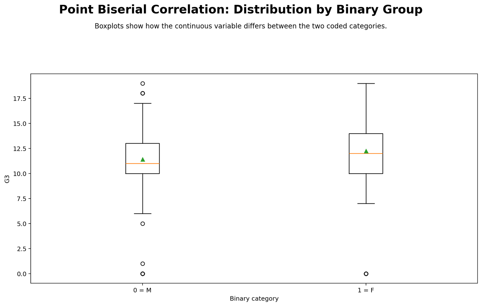
The boxplot shows the distribution of G3 separately for the F-coded group and the M-coded group. The F group has a slightly higher center than the M group. This matches the verified means: F has mean G3 = 12.2533, while M has mean G3 = 11.4060.
The most important feature of the chart is overlap. The boxes and whiskers are not widely separated. Many students in both groups have similar final grades. This visual pattern explains why the coefficient is small even though the p-value is significant. A strong point-biserial relationship would show much clearer separation between the two groups.
The chart also helps prevent overstatement. The result does not mean one group always scores higher than the other. It only means that, on average, the group coded 1 has a lower G3 score in this dataset.
Python Chart 2: Group Means with 95% Confidence Intervals
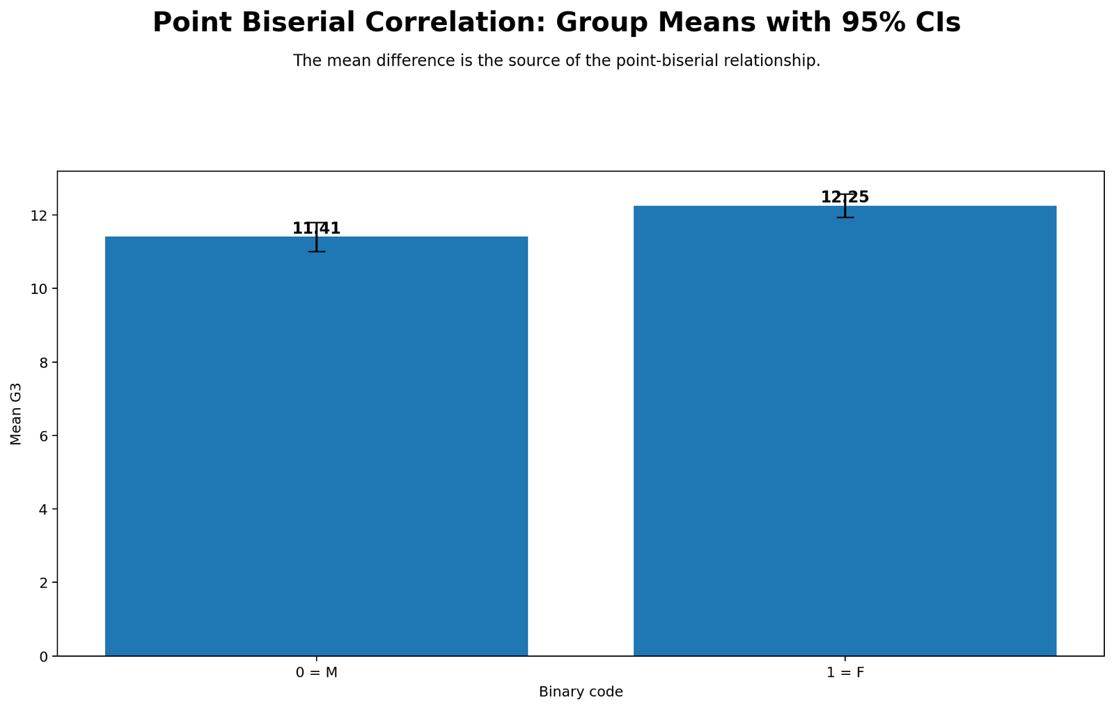
The group means chart makes the direction of the result easy to see. The F-coded group has a higher mean G3 score, and the M-coded group has a lower mean G3 score. The mean difference is -0.847249 when calculated as M minus F.
This is the chart that most directly explains the negative sign. Since M is coded 1 and M has the lower mean, the coefficient is negative. If the coding were reversed, the line or bars would represent the same group difference but the sign of the correlation would reverse.
The confidence intervals help readers understand sampling uncertainty. Because N is large, the group means are estimated fairly precisely. Still, the actual mean gap is less than one grade point, so the practical effect remains small.
Python Chart 3: Point Biserial Report Card
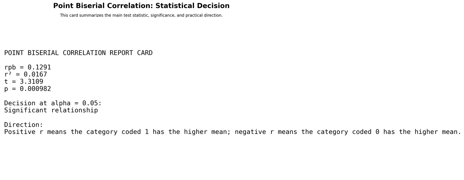
The report card gives the final result in one place: binary variable sex, continuous variable G3, N = 649, F coded 0, M coded 1, rpb = -0.129077, t(647) = -3.310938, p = 0.000982, and a significant decision at α = .05.
This is the best chart to use when writing the final results paragraph because it contains the coefficient and the test statistic. However, the report card should still be interpreted with the distribution and mean charts. The p-value tells us the association is statistically detectable, while the coefficient tells us the effect is small.
Python Chart 4: Histogram Overlay by Binary Group
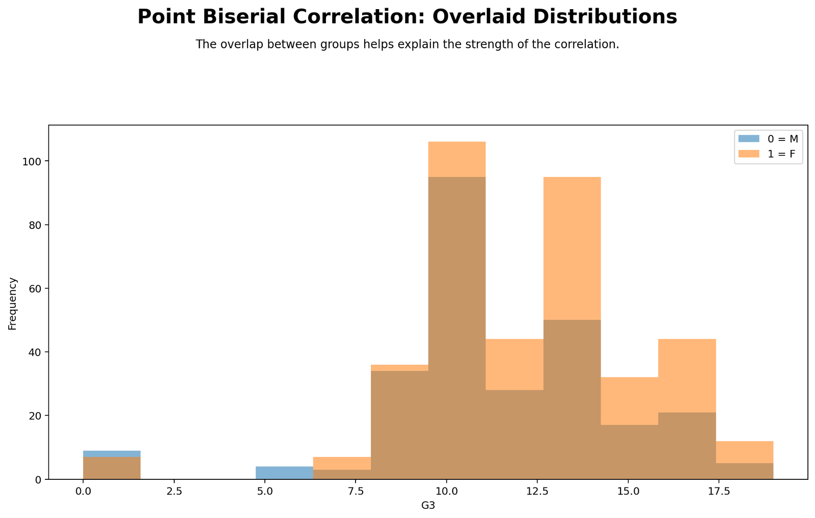
The histogram overlay shows how the full G3 distribution differs across the two binary groups. The two distributions overlap heavily, which confirms that the association is not large. The F-coded distribution is slightly shifted toward higher final grades, while the M-coded distribution has relatively more lower-grade observations.
This chart is helpful because a boxplot summarizes distribution shape, but a histogram shows the frequency pattern across grade values. The overlap demonstrates why the practical effect should not be exaggerated. A statistically significant point-biserial correlation can still be small when group distributions largely overlap.
Python Chart 5: Binary Scatter with Fitted Line
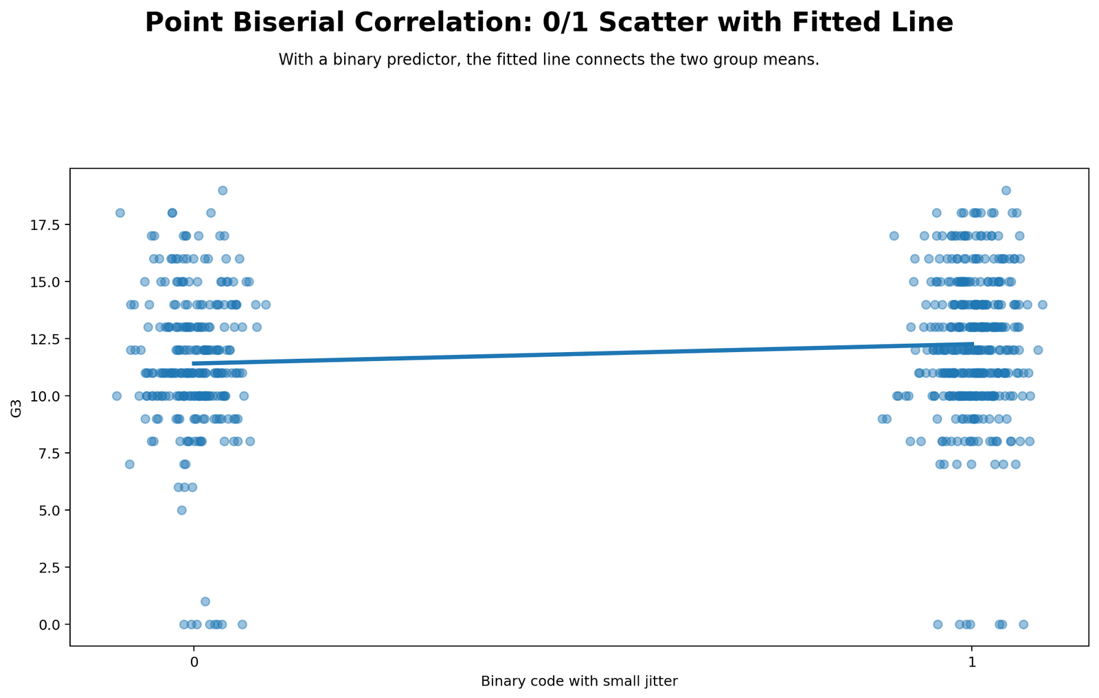
The binary scatterplot places the coded binary variable on the x-axis and G3 on the y-axis. Because the x-axis has only two possible values, points stack at 0 and 1. Jittering or transparency helps show the density of observations.
The fitted line slopes downward because the group coded 1 has a lower mean G3 score. The slope is not steep, which visually matches the small value of rpb. This chart is useful for connecting point-biserial correlation with ordinary Pearson correlation and simple linear regression. With a 0/1 predictor, the fitted-line difference corresponds to the group mean difference.
R Chart-by-Chart Interpretation
The R charts validate the Python results using a separate workflow and colorful chart versions. The same five visuals are repeated: boxplot, group means with confidence intervals, report card, histogram overlay, and binary scatter with fitted line.
R Chart 1: Colorful Distribution by Binary Group Boxplot
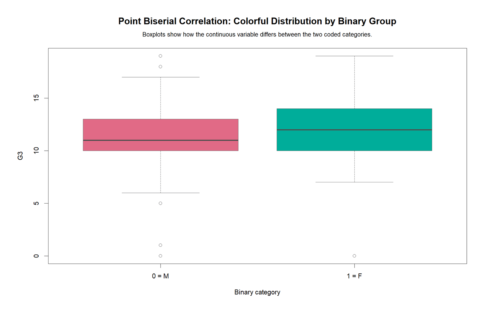
The R boxplot confirms the same distribution pattern as Python. The F group has a slightly higher central tendency than the M group, but the distributions overlap strongly. This independent software validation supports the same interpretation.
R Chart 2: Colorful Group Means with 95% Confidence Intervals
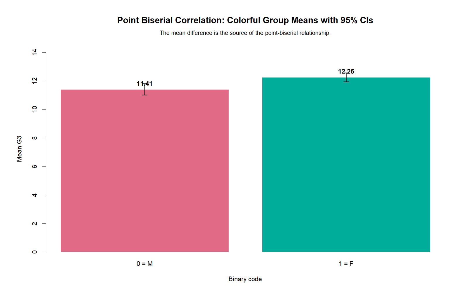
The R group means chart validates the same mean difference: the F group has a higher mean G3 score than the M group. The sign of rpb is negative because M is coded 1 and the M group mean is lower.
R Chart 3: Colorful Point Biserial Report Card
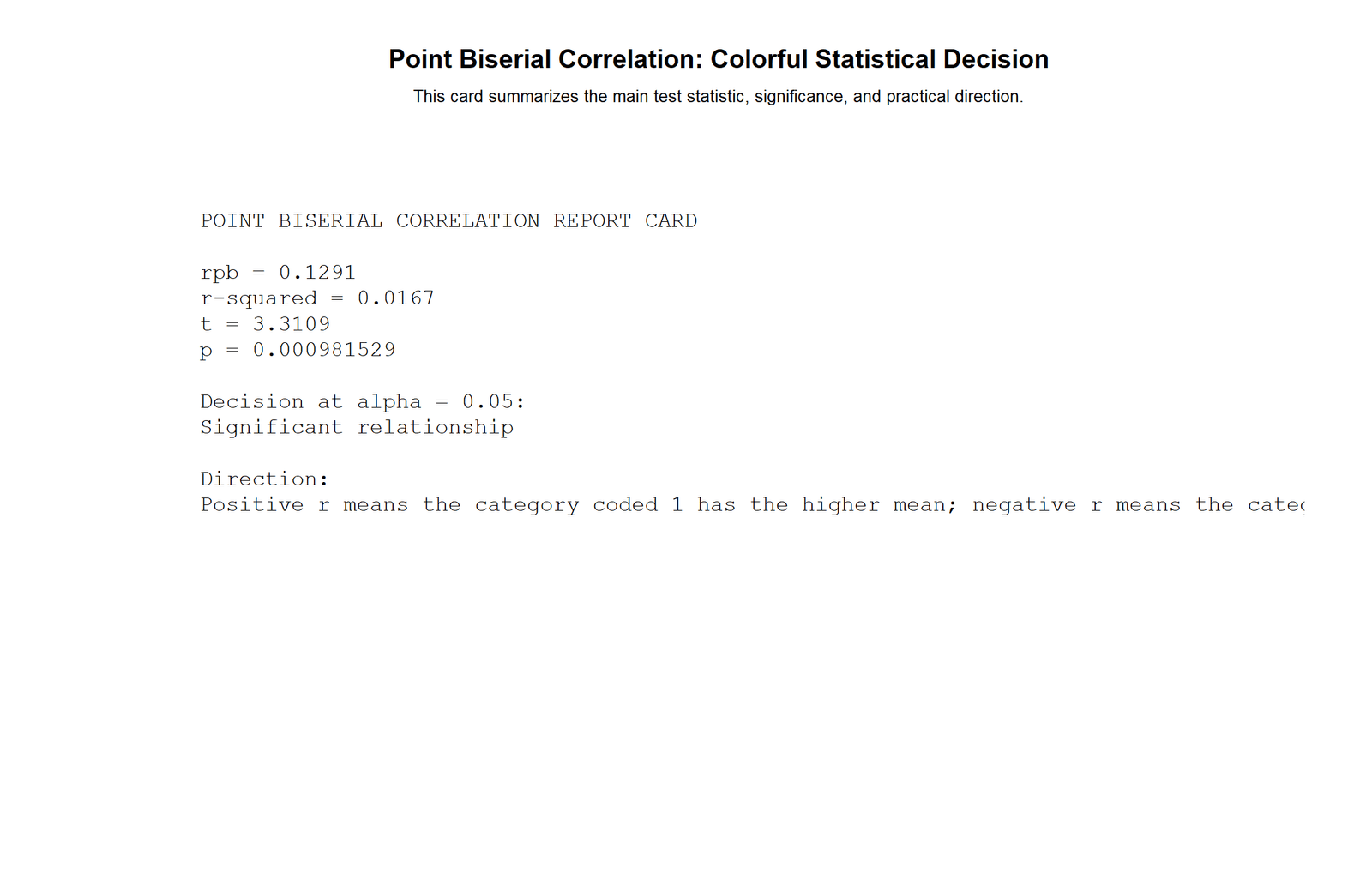
The R report card confirms the same final statistics: N = 649, rpb ≈ -0.129, t ≈ -3.311, p ≈ .001, and a significant decision. The chart is useful because it confirms that the result does not depend on one software environment.
R Chart 4: Colorful Histogram Overlay by Binary Group
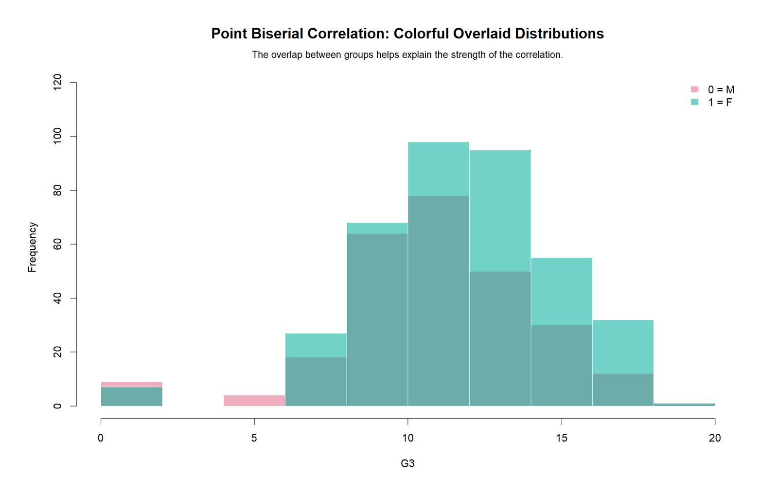
The R histogram overlay again shows heavy overlap between the two G3 distributions. This supports the small-effect conclusion. The chart is especially useful for students who might otherwise interpret statistical significance as a large practical difference.
R Chart 5: Colorful Binary Scatter with Fitted Line
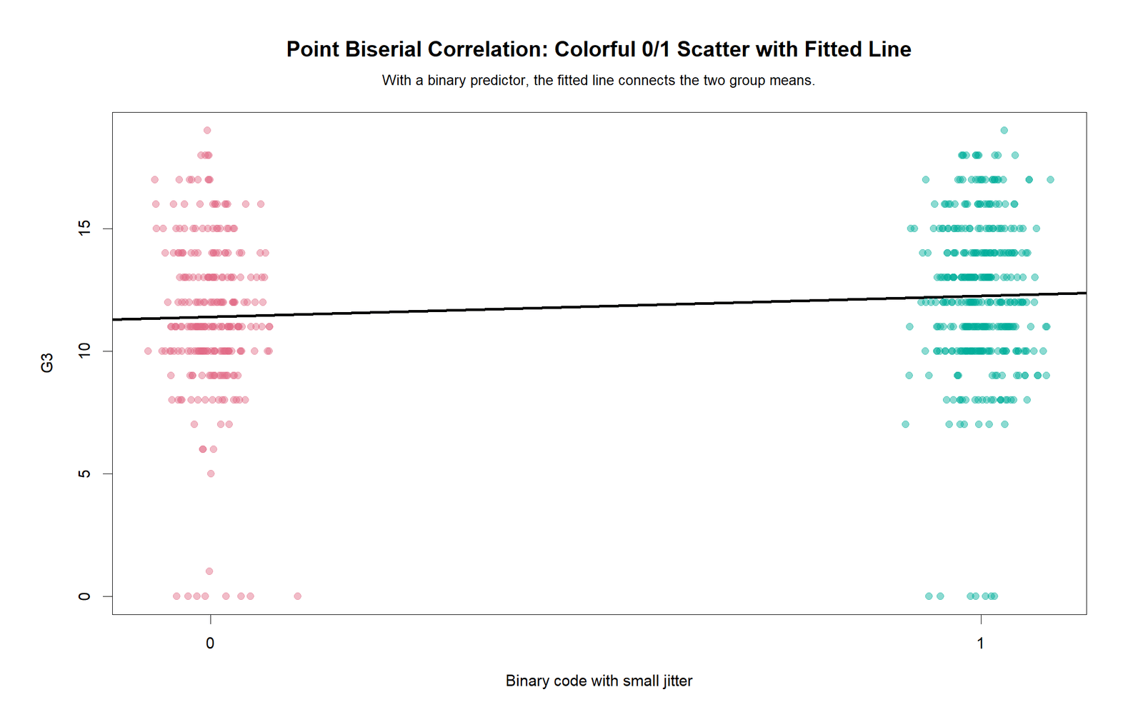
The R fitted-line chart confirms the negative direction. The line decreases from code 0 to code 1 because the M-coded group has the lower mean. The decline is visible but not steep, which matches the small magnitude of the point-biserial coefficient.
SPSS Output Interpretation
The SPSS output is included for formal reporting. In SPSS, Point Biserial Correlation can be obtained by recoding the binary variable into 0 and 1 and then running a Pearson correlation between the binary code and the continuous variable. It can also be interpreted alongside an independent-samples t-test because both methods describe the same two-group mean difference from different perspectives.
Open the SPSS Point Biserial Correlation Output PDF
| SPSS Output Item | Expected Value / Meaning | How to Interpret It |
|---|---|---|
| Binary coding | F = 0, M = 1 | The sign of r depends on this coding. |
| Continuous variable | G3 | Final grade score. |
| Valid N | 649 | Complete cases used in the analysis. |
| Pearson correlation with binary code | r = -0.129 | This is the point-biserial coefficient. |
| Sig. two-tailed | p ≈ .001 | The association is statistically significant. |
| Independent-samples t-test context | t(647) ≈ -3.311 | Matches the correlation significance logic. |
| Group means | F mean higher than M mean | Explains the negative sign when M is coded 1. |
SPSS users should avoid reporting only the correlation table. A clear report should also mention the group means. Without the means and coding direction, readers may misunderstand why the coefficient is negative.
Excel Worked File Explanation
The Excel workbook gives a fully worked Point Biserial Correlation example. It includes raw data, encoded variables, the main worked example, pairwise point-biserial screening, Excel method notes and a dashboard. The workbook is useful for students because it shows both the direct Excel correlation method and the manual formula using group means.
Download the Point Biserial Correlation Fully Worked Excel File
| Excel Sheet | Purpose | What It Teaches |
|---|---|---|
| Read_Me | Explains the workbook setup. | Shows project folder, dataset size, main variables and method note. |
| Raw_Data | Stores the full dataset. | Allows users to verify the original student performance variables. |
| Encoded_Worked | Creates the binary code and continuous variable columns. | Shows sex coded F=0 and M=1 with G3 as the outcome. |
| Main_Worked_Example | Shows the main formula calculation. | Calculates N, group sizes, group means, SD, r, r², t, df and p-value. |
| Pairwise_Results | Ranks binary-continuous relationships. | Shows top point-biserial relationships across multiple variables. |
| Excel_Method | Explains formula steps. | Documents CORREL, mean-difference formula and T.DIST.2T p-value method. |
| Dashboard | Summarizes the main result. | Shows key metrics, group means and top-ranked pairwise results. |
Excel Main Worked Example
The workbook uses G3 as the continuous variable and sex as the binary variable. The coding rule is F = 0 and M = 1. The direct Excel method is:
The formula-driven Excel result is -0.1290774866. The manual group-means formula gives the same value, confirming the calculation. The t statistic is -3.3109376930, df is 647, and the two-tailed p-value is 0.0009815287.
Excel Interpretation Rule
Excel makes the coding direction very clear. Since the binary code is F=0 and M=1, a negative coefficient means the M group has a lower mean. It does not mean the variable is “bad,” and it does not automatically imply a large effect. It only describes the direction of the mean difference under the chosen coding.
Excel teaching value: The workbook is not only a result file. It shows the full chain from binary coding to group means, direct CORREL calculation, manual formula, t statistic, p-value, decision and pairwise screening.
Python, R, SPSS and Excel Workflows
The same Point Biserial Correlation analysis can be reproduced in Python, R, SPSS and Excel. The steps are similar in every tool: code the binary variable, choose the continuous variable, compute the correlation, check group means, run the significance test and interpret the effect size.
| Software | Main Workflow | Best Use |
|---|---|---|
| Python | Use pandas for binary coding, scipy for Pearson/point-biserial correlation and matplotlib for boxplots, means, histograms and scatterplots. | Automated reporting, charts and reproducible analysis. |
| R | Use cor.test() after coding the binary variable as 0/1, t.test() for mean-difference context and charting functions for validation. | Statistical validation and colorful publication visuals. |
| SPSS | Recode binary variable to 0/1, run Pearson correlation with G3 and add independent-samples t-test for group means. | Formal output PDF and academic reporting. |
| Excel | Use CORREL, AVERAGEIF, STDEV.S, COUNTIF, T.DIST.2T and formula-driven summary tables. | Transparent formula teaching and workbook-based learning. |
Code Blocks and Excel Formulas
Python Code for Point Biserial Correlation
import pandas as pd
import numpy as np
from scipy import stats

# Load data
df = pd.read_csv("dataset.csv")

# Main worked example
continuous_var = "G3"
binary_var = "sex"

work = df[[binary_var, continuous_var]].dropna().copy()
work[continuous_var] = pd.to_numeric(work[continuous_var], errors="coerce")

# Code F = 0 and M = 1
work["binary_code"] = work[binary_var].map({"F": 0, "M": 1})
work = work.dropna()

x = work["binary_code"].to_numpy()
y = work[continuous_var].to_numpy()
n = len(work)

# Point-biserial correlation is Pearson correlation with a 0/1 variable
r_pb, p_value = stats.pearsonr(x, y)

# Group means
n0 = int((x == 0).sum())
n1 = int((x == 1).sum())
mean0 = y[x == 0].mean()
mean1 = y[x == 1].mean()
sd_y = y.std(ddof=1)

# Manual formula
r_manual = ((mean1 - mean0) / sd_y) * np.sqrt((n0 * n1) / (n * (n - 1)))

# t statistic and r squared
t_value = r_pb * np.sqrt((n - 2) / (1 - r_pb**2))
df_t = n - 2
r_squared = r_pb**2

print("N:", n)
print("n0:", n0, "n1:", n1)
print("Mean code 0:", mean0)
print("Mean code 1:", mean1)
print("Mean difference 1-0:", mean1 - mean0)
print("Point-biserial r:", r_pb)
print("Manual r:", r_manual)
print("r squared:", r_squared)
print("t:", t_value, "df:", df_t, "p:", p_value)
R Code for Point Biserial Correlation
# Load data
df <- read.csv("dataset.csv", stringsAsFactors = FALSE)

# Main worked example
work <- na.omit(df[, c("sex", "G3")])
work$G3 <- as.numeric(work$G3)

# Code F = 0 and M = 1
work$sex_code <- ifelse(work$sex == "M", 1, 0)

# Point-biserial correlation is Pearson correlation with a 0/1 variable
cor_result <- cor.test(work$sex_code, work$G3, method = "pearson")
print(cor_result)

# Group summaries
n <- nrow(work)
n0 <- sum(work$sex_code == 0)
n1 <- sum(work$sex_code == 1)
mean0 <- mean(work$G3[work$sex_code == 0])
mean1 <- mean(work$G3[work$sex_code == 1])
sd_y <- sd(work$G3)

r_manual <- ((mean1 - mean0) / sd_y) * sqrt((n0 * n1) / (n * (n - 1)))
t_value <- unname(cor_result$estimate) * sqrt((n - 2) / (1 - unname(cor_result$estimate)^2))
r_squared <- unname(cor_result$estimate)^2

cat("N =", n, "\n")
cat("n0 =", n0, "n1 =", n1, "\n")
cat("Mean code 0 =", mean0, "\n")
cat("Mean code 1 =", mean1, "\n")
cat("Manual point-biserial r =", r_manual, "\n")
cat("t =", t_value, "\n")
cat("r squared =", r_squared, "\n")

# Mean difference context
t.test(G3 ~ sex_code, data = work, var.equal = TRUE)
SPSS Syntax for Point Biserial Correlation
* Point Biserial Correlation in SPSS.
* Binary variable: sex coded F=0 and M=1.
* Continuous variable: G3.

OUTPUT CLOSE ALL.
OUTPUT NEW NAME=Point_Biserial_Output.

RECODE sex ('F'=0) ('M'=1) INTO sex_code.
VARIABLE LABELS sex_code 'Sex coded for point-biserial correlation: F=0, M=1'.
VALUE LABELS sex_code 0 'F' 1 'M'.
EXECUTE.

FREQUENCIES VARIABLES=sex sex_code.
DESCRIPTIVES VARIABLES=G3 sex_code
  /STATISTICS=MEAN STDDEV MIN MAX.

CORRELATIONS
  /VARIABLES=sex_code G3
  /PRINT=TWOTAIL
  /MISSING=PAIRWISE.

T-TEST GROUPS=sex_code(0 1)
  /VARIABLES=G3
  /CRITERIA=CI(.95).

EXAMINE VARIABLES=G3 BY sex_code
  /PLOT BOXPLOT HISTOGRAM NPPLOT
  /STATISTICS DESCRIPTIVES
  /CINTERVAL 95
  /MISSING LISTWISE.

OUTPUT EXPORT
  /CONTENTS EXPORT=VISIBLE
  /PDF DOCUMENTFILE='Point-Biserial-Correlation-SPSS-Output.pdf'.
Excel Formulas for Point Biserial Correlation
Assume:
continuous_range = G3 values
binary_range = 0/1 coding for sex

N:
=COUNT(continuous_range)

n0:
=COUNTIF(binary_range,0)

n1:
=COUNTIF(binary_range,1)

Mean for code 0:
=AVERAGEIF(binary_range,0,continuous_range)

Mean for code 1:
=AVERAGEIF(binary_range,1,continuous_range)

Sample SD of continuous variable:
=STDEV.S(continuous_range)

Direct point-biserial correlation:
=CORREL(continuous_range,binary_range)

Manual point-biserial formula:
=((Mean1-Mean0)/SD_Y)*SQRT((n0*n1)/(N*(N-1)))

r squared:
=r_pb^2

t statistic:
=r_pb*SQRT((N-2)/(1-r_pb^2))

Degrees of freedom:
=N-2

Two-tailed p-value:
=T.DIST.2T(ABS(t),df)

Decision:
=IF(p_value<0.05,"Significant at alpha = 0.05","Not significant at alpha = 0.05")
Assumptions and Data Checks
Point Biserial Correlation is closely related to Pearson correlation and the independent-samples t-test. It does not require both variables to be continuous, but it does require one true binary variable and one continuous outcome. The observations should be independent, and the continuous outcome should be interpreted sensibly within each group.
| Check | Why It Matters | Status in This Example |
|---|---|---|
| One variable is true binary | Point-biserial requires a real two-category variable. | sex has two groups: F and M. |
| One variable is continuous | The outcome should be numeric and meaningful. | G3 is a numeric final grade score. |
| Binary coding is clear | The sign depends on which group is coded 1. | F=0 and M=1 are explicitly stated. |
| Independent observations | Each row should represent a separate student/case. | The dataset treats each student as one observation. |
| Group distribution checked | Outliers or very uneven distributions can affect interpretation. | Boxplots and histograms are included. |
| Effect size reported | p-value alone does not show practical strength. | rpb and r² are reported. |
| No causal claim | Correlation does not prove cause and effect. | The result is reported as association only. |
The main caution is effect-size interpretation. Since rpb is only -0.129, the result is small even though it is statistically significant. This is a common situation in large datasets.
How to Report Point Biserial Correlation
A complete report should include the binary coding, continuous variable, group means, sample size, coefficient, t statistic, degrees of freedom, p-value, effect-size strength and interpretation of direction.
APA-Style Full Report
A point-biserial correlation was computed to examine the association between sex coding and G3 final grade. Sex was coded as F = 0 and M = 1. The analysis included 649 students, with 383 students in the F group and 266 students in the M group. The F group had a higher mean G3 score (M = 12.253) than the M group (M = 11.406). The point-biserial correlation was statistically significant and small, rpb = -.129, r² = .017, t(647) = -3.311, p = .001. Because the M group was coded as 1 and had the lower mean, the coefficient was negative.
Short APA-Style Version
A small but statistically significant point-biserial association was found between sex coding and G3 final grade, rpb = -.129, t(647) = -3.311, p = .001. The negative sign reflects the coding direction because M was coded as 1 and had a lower mean G3 score than F.
Plain-Language Version
Students in the F-coded group had a slightly higher average G3 final grade than students in the M-coded group. The difference was statistically significant, but the relationship was small, so it should not be described as a strong group difference.
Common Mistakes in Point Biserial Correlation Interpretation
| Mistake | Why It Is a Problem | Better Practice |
|---|---|---|
| Calling it biserial correlation without checking the binary variable | Point-biserial is for true binary variables; biserial is for artificial dichotomies. | Use point-biserial when the binary variable is naturally two categories. |
| Ignoring coding direction | The sign changes when 0 and 1 are reversed. | Always state which group is coded 1. |
| Reporting only the p-value | The p-value does not show strength. | Report rpb, r² and group means. |
| Calling a small significant result strong | Large samples can make small effects statistically significant. | Use small/moderate/large effect-size wording. |
| Using point-biserial for two binary variables | That situation is a 2x2 contingency table. | Use Phi Coefficient or chi-square. |
| Using it when the continuous variable is actually ordinal with few levels | The numeric distances may not be meaningful. | Consider rank or ordinal methods if the outcome is ordinal. |
| Claiming causation | Correlation does not prove cause and effect. | Use association wording unless the study design supports causal inference. |
Downloads and Resources
Download R Report PDFR validation report with colorful point-biserial charts.
Download SPSS Output PDFSPSS correlation and t-test context output for point-biserial interpretation.
Download Excel Worked FileFully worked Excel workbook with direct CORREL method, manual formula, t statistic and pairwise results.
External References
For additional learning, review documentation and references on Pearson correlation, point-biserial correlation, independent-samples t-test, binary coding, effect size interpretation and confidence intervals. These topics are commonly taught together because point-biserial correlation is the correlation form of a two-group mean comparison.
FAQs About Point Biserial Correlation
What is Point Biserial Correlation in simple words?
Point Biserial Correlation measures the relationship between a true two-category variable and a continuous variable. It is Pearson correlation when the binary variable is coded 0 and 1.
What was the main result in this guide?
The main result was sex coded F=0 and M=1 correlated with G3 final grade. The result was rpb = -0.129077, t(647) = -3.310938, p = 0.000982, N = 649. The effect was statistically significant but small.
Why is the coefficient negative?
The coefficient is negative because M was coded as 1 and the M group had a lower mean G3 score than the F group. Reversing the coding would reverse the sign.
Is Point Biserial Correlation the same as Pearson correlation?
Yes, mathematically it is Pearson correlation when one variable is coded 0 and 1. The special name is used because one variable is binary and the interpretation focuses on group mean differences.
What is the difference between point-biserial and biserial correlation?
Point-biserial correlation is used for true binary variables. Biserial correlation is used when the binary variable is an artificial split from an underlying continuous or latent variable.
How do I calculate Point Biserial Correlation in Excel?
Code the binary variable as 0 and 1, then use CORREL(continuous_range, binary_code_range). You can also use the group-means formula with group means, standard deviation and group sizes.
How do I run Point Biserial Correlation in SPSS?
Recode the binary variable to 0 and 1, then run Pearson correlation between the binary code and the continuous variable. Add an independent-samples t-test to show the group mean difference.
What does r squared mean for Point Biserial Correlation?
r squared shows the proportion of variance in the continuous variable associated with the binary coding. In this guide, r² = 0.016661, meaning about 1.67% of G3 variance is associated with sex coding.
Can I use Point Biserial Correlation when both variables are binary?
No. If both variables are binary, use Phi Coefficient or a chi-square test for a 2x2 table.
Does a significant Point Biserial Correlation prove causation?
No. Point Biserial Correlation shows association, not cause and effect. The result should be interpreted as a small association between sex coding and G3, not as a causal claim.
How should I report the result in one sentence?
You can write: “A small but statistically significant point-biserial association was found between sex coding and G3 final grade, rpb = -.129, t(647) = -3.311, p = .001.”

