
Correlation, Binary Groups, Point-Biserial Comparison and Excel Worked Results
Biserial Correlation: Formula, Interpretation, SPSS, Python, R and Excel Guide
Biserial Correlation estimates the relationship between a continuous variable and a binary variable that represents an artificial split of an underlying continuous trait. This guide also explains point-biserial correlation, because many real data examples use a true binary group such as sex, pass/fail or yes/no. You will learn the formula, assumptions, SPSS output interpretation, Python chart interpretation, R validation charts, Excel worked formulas, APA reporting wording, common mistakes, internal resources and downloadable files.
Quick Answer: Biserial Correlation Result
The main SPSS, Python and R report tested the association between sex and G3 final grade. The binary variable was coded F = 0 and M = 1. The continuous variable was G3. The sample contained N = 649 students, with 383 students in the F group and 266 students in the M group.
The group means showed that the F group had a higher mean G3 score (M = 12.25) than the M group (M = 11.41). Because M was coded as 1 and M had the lower mean, the coefficient was negative. The point-biserial result was r = -0.1291, with a 95% confidence interval from approximately -0.2040 to -0.0526. The test statistic was t(647) = -3.3109, with p = .000982. The normal-cut corrected biserial estimate was rb = -0.1632.
Final interpretation: The main report shows a statistically significant but small negative association between the sex coding variable and G3. Since M was coded 1 and had the lower group mean, the negative sign means the M-coded group scored lower on average. The practical effect is small because the two distributions overlap strongly even though the p-value is below .05.
Important distinction: For a true binary variable such as sex, the point-biserial correlation is usually the primary coefficient. Biserial correlation is most appropriate when the binary variable is an artificial dichotomy of an underlying continuous variable. That is why the Excel workbook also includes a stronger worked example using G1 dichotomized at 10 against continuous G3.
Table of Contents
- What Is Biserial Correlation?
- Biserial vs Point-Biserial vs Rank-Biserial
- Biserial Correlation Formula
- Null and Alternative Hypotheses
- Dataset and Variables Used
- SPSS Output Interpretation
- Python Chart-by-Chart Interpretation
- R Chart-by-Chart Validation
- Excel Results Explained
- SPSS, R, Python and Excel Workflows
- Code Blocks for Biserial Correlation
- APA Reporting Wording
- Common Mistakes
- When to Use Biserial Correlation
- Downloads and Resources
- Related Guides
- FAQs
What Is Biserial Correlation?
Biserial correlation is a correlation coefficient used when one variable is continuous and the other variable is binary because it has been cut from an underlying continuous or normally distributed trait. The word “biserial” means the analysis has one continuous series and one two-category series. The two-category series is treated as a thresholded version of something more continuous.
For example, suppose a researcher turns an exam score into a pass/fail variable using a cutoff of 10. The pass/fail variable has only two categories, but it was created from a continuous score. In that situation, the biserial correlation estimates what the relationship would look like before the continuous variable was split into two groups.
In contrast, if the binary variable is naturally binary, such as yes/no, present/absent, treatment/control or female/male coding, the point-biserial correlation is usually the cleaner coefficient. The point-biserial coefficient is simply the Pearson correlation between a 0/1 binary variable and a continuous variable. It is closely related to an independent-samples Student’s t-test, two-sample t-test and effect size reporting.
Simple definition: Biserial correlation estimates the relationship between a continuous outcome and an artificially dichotomized predictor. Point-biserial correlation measures the observed relationship between a continuous variable and a true 0/1 binary variable.
Biserial vs Point-Biserial vs Rank-Biserial Correlation
Many students search for biserial and point biserial correlation together because the names sound similar. They are connected, but they are not the same. The most important decision is whether the binary variable is naturally binary or artificially dichotomized.
| Coefficient | Use It When | Example | Main Interpretation |
|---|---|---|---|
| Point-biserial correlation | One variable is truly binary and the other is continuous. | Sex coded 0/1 with G3 score. | Observed Pearson correlation between binary coding and continuous score. |
| Biserial correlation | The binary variable is an artificial cut of an underlying continuous trait. | G1 converted to low/high using G1 >= 10. | Estimated correlation before the split, adjusted for the normal cutoff. |
| Rank-biserial correlation | The analysis is based on ranks or Mann-Whitney style group comparison. | Two groups compared on an ordinal or non-normal outcome. | Nonparametric effect size based on ranks, not raw normal correlation. |
| Pearson correlation | Both variables are continuous. | G1 and G3 as numeric grade scores. | Linear association between two continuous variables. |
Better reporting rule: Do not call every binary-continuous correlation a biserial correlation. If the binary variable is true binary, report point-biserial r. If the binary variable is an artificial cut from a continuous or latent variable, report biserial r and explain the cutoff.
Biserial Correlation Formula
The point-biserial formula uses the difference between two group means, the standard deviation of the continuous variable and the proportions in the two binary groups:
The biserial formula adds a correction for the normal cutoff that produced the binary groups:
| Symbol | Meaning | How It Is Used |
|---|---|---|
| M1 | Mean of the continuous variable for group coded 1 | For the main report, the M group was coded 1 and had mean G3 = 11.41. |
| M0 | Mean of the continuous variable for group coded 0 | For the main report, the F group was coded 0 and had mean G3 = 12.25. |
| SDY | Standard deviation of the continuous variable | G3 had SD ≈ 3.231 in the full sample. |
| p | Proportion in group 1 | For the main report, p ≈ .410 for the M group. |
| q | Proportion in group 0 | For the main report, q ≈ .590 for the F group. |
| y | Height of the standard normal curve at the cutoff | Used only in the biserial correction. |
The significance test is usually based on the observed point-biserial correlation because it is a standard Pearson correlation with a 0/1 variable. The common t formula is:
For the main report, this gives t(647) = -3.3109 and p = .000982. You can connect this interpretation with p-value, confidence interval, standard deviation and standard error guides.
Null and Alternative Hypotheses for Biserial Correlation
The hypothesis statement depends on whether the researcher is emphasizing the observed point-biserial association or the normal-cut corrected biserial estimate. In applied reports, the p-value is commonly tied to the point-biserial test.
| Statement | Hypothesis | Meaning |
|---|---|---|
| Null hypothesis | H0: ρpb = 0 | The binary variable and continuous variable have no linear association in the population. |
| Alternative hypothesis | H1: ρpb ≠ 0 | The binary variable and continuous variable are associated in the population. |
| Biserial interpretation | ρb ≠ 0 | The underlying continuous trait behind the artificial split is related to the continuous outcome. |
Decision for the main report: Because p = .000982 is below .05, the null hypothesis of no observed point-biserial association is rejected. The direction is negative only because M was coded as 1 and the M group had a lower mean G3 score than the F group.
Dataset and Variables Used
The main SPSS, Python and R charts use the student performance dataset with G3 final grade as the continuous variable and sex as the binary grouping variable. The report coded F = 0 and M = 1. This example is excellent for teaching the difference between point-biserial and biserial correlation because sex is a true binary group, while the Excel workbook also includes an artificial dichotomy example using G1 >= 10.
| Variable | Role | Used In | Interpretation Purpose |
|---|---|---|---|
| G3 | Continuous outcome | SPSS, Python, R and Excel | Final grade score being compared between groups. |
| sex | True binary variable | Main SPSS/Python/R report | Used for point-biserial and educational biserial comparison. |
| G1 >= 10 | Artificial dichotomy | Excel workbook | Better example of true biserial logic because G1 was originally numeric. |
| G2 >= median | Artificial dichotomy | Excel results table | Strongest median-split biserial relationship with G3 in the workbook. |
Before reporting the coefficient, it is useful to check descriptive statistics, frequency distributions, histograms, box plots, null and alternative hypotheses and parametric vs nonparametric tests.
SPSS Output Interpretation for Biserial Correlation
The SPSS output verifies the main binary-continuous result. The binary grouping variable has 383 F cases and 266 M cases, with no missing cases in the valid analysis. The continuous G3 score has N = 649, minimum 0, maximum 19, mean approximately 11.91 and standard deviation approximately 3.231.
Open the SPSS Biserial Correlation output PDF
| SPSS Output Item | Value | Interpretation |
|---|---|---|
| Valid N | 649 | The same 649 students were used for the binary grouping and continuous score. |
| Group 0 | F, n = 383, 59.0% | This is the reference group in the 0/1 coding. |
| Group 1 | M, n = 266, 41.0% | This group receives the value 1, so a lower mean creates a negative coefficient. |
| F group mean | 12.25 | The F group had the higher average final grade. |
| M group mean | 11.41 | The M group had the lower average final grade. |
| Mean difference | 0.847 | The group gap is statistically significant but modest in grade-score units. |
| Levene’s test | F = .004, p = .950 | The equal-variances assumption is not a major concern for the t-test context. |
| Independent-samples t-test | t(647) = 3.311, p = .001 | Equivalent mean-difference evidence supports the point-biserial result. |
| Point-biserial r | -0.129 | Small negative association due to M being coded 1 and having lower mean G3. |
| Biserial r | -0.163 | Normal-cut corrected estimate, larger in magnitude than point-biserial r. |
SPSS Interpretation Summary
The SPSS result should be reported as a small but statistically significant binary-continuous association. The sign is a coding sign, not a value judgment: because M was coded 1 and the M mean was lower, the coefficient is negative. If the coding were reversed, the sign would become positive while the strength would remain the same.
SPSS reporting note: When the binary variable is truly binary, report the point-biserial result as the main correlation. Mention the biserial estimate only if you are intentionally applying a normal-cut correction or teaching the difference between point-biserial and biserial correlation.
Python Chart-by-Chart Interpretation
The Python charts show how the coefficient is built from group distributions, group means, coefficient comparison and a one-page report card. The charts are useful because they show why a statistically significant p-value can still represent a small practical association.
Python Chart 1: Continuous Scores by Binary Group
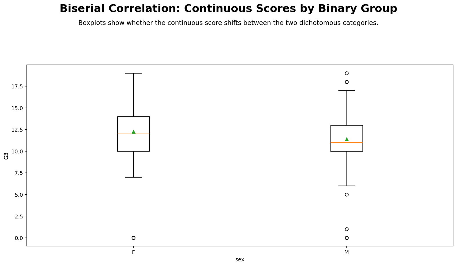
This chart shows the G3 distribution separately for F and M. The F group has a slightly higher center than the M group, with the F median around 12 and the M median around 11. The boxes still overlap strongly, which means the association is not large even though the mean difference is statistically significant. The F group has one very low outlier at 0, while the M group shows several low outliers near 0 or 1 and a few high values near 18 to 19.
The chart explains why the point-biserial coefficient is small. The two groups do not form clearly separated distributions. Instead, most scores occupy the same broad grade range, with only a modest downward shift for the M-coded group. This is exactly the pattern that produces a small negative correlation such as r = -0.129.
Python Chart 2: Group Mean Difference
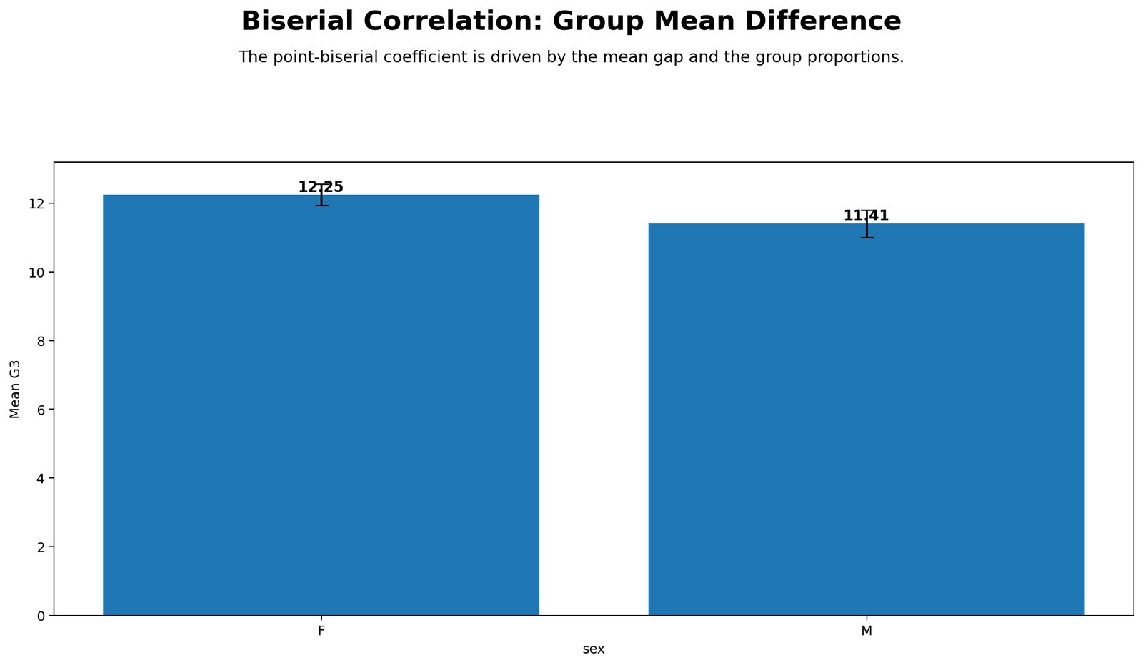
The mean chart gives the clearest numerical story. The F group mean is labeled about 12.25, while the M group mean is about 11.41. The difference is roughly 0.85 grade points. The error bars are small because the sample is large, so even this modest group gap becomes statistically significant.
This chart should be read together with the boxplot. The mean gap is real, but the distributions overlap. Therefore, the best conclusion is not “the groups are very different.” The better conclusion is that the F-coded group scored slightly higher on average, producing a statistically significant but small point-biserial association.
Python Chart 3: Point-Biserial vs Biserial Coefficient
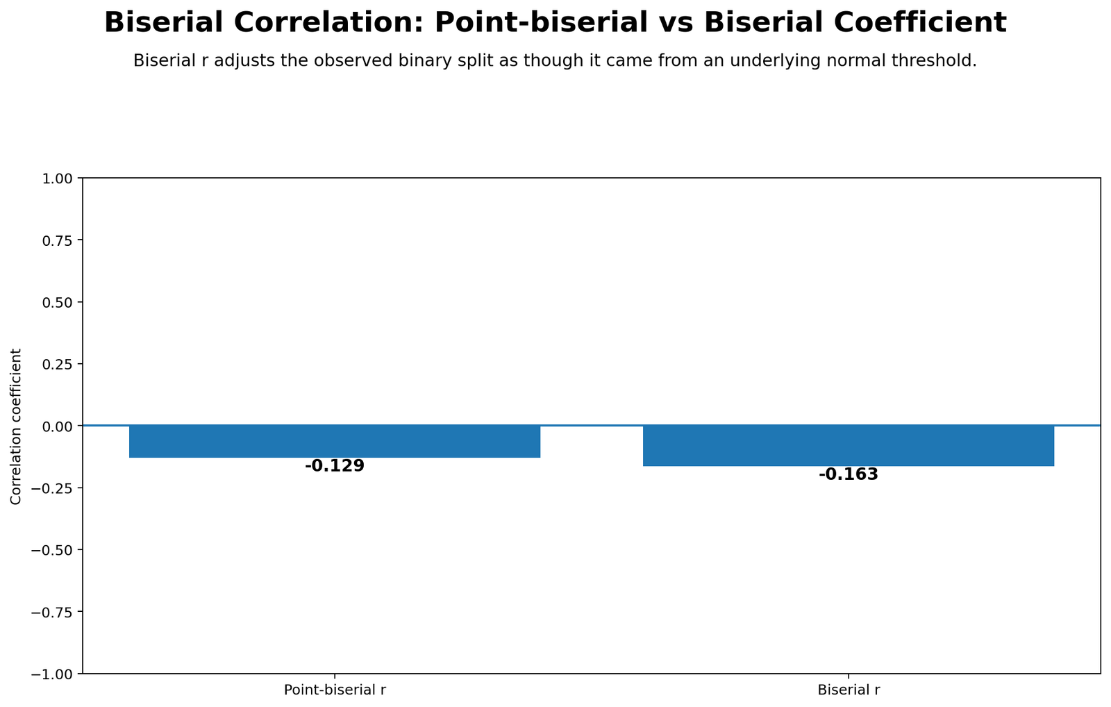
This chart shows two coefficient bars below zero. The point-biserial coefficient is labeled -0.129, and the biserial coefficient is labeled -0.163. Both signs are negative because the group coded 1 has the lower G3 mean. The biserial estimate is larger in magnitude because it adjusts the observed 0/1 split as though it came from an underlying normal threshold.
The chart is especially useful for explaining the difference between the two coefficients. Point-biserial r is the direct observed correlation with the coded binary variable. Biserial r is an adjusted estimate. Since sex is a true binary variable, the point-biserial value is the cleaner main report statistic, while the biserial value is useful as a demonstration of the correction.
Python Chart 4: Jittered Binary Scatter
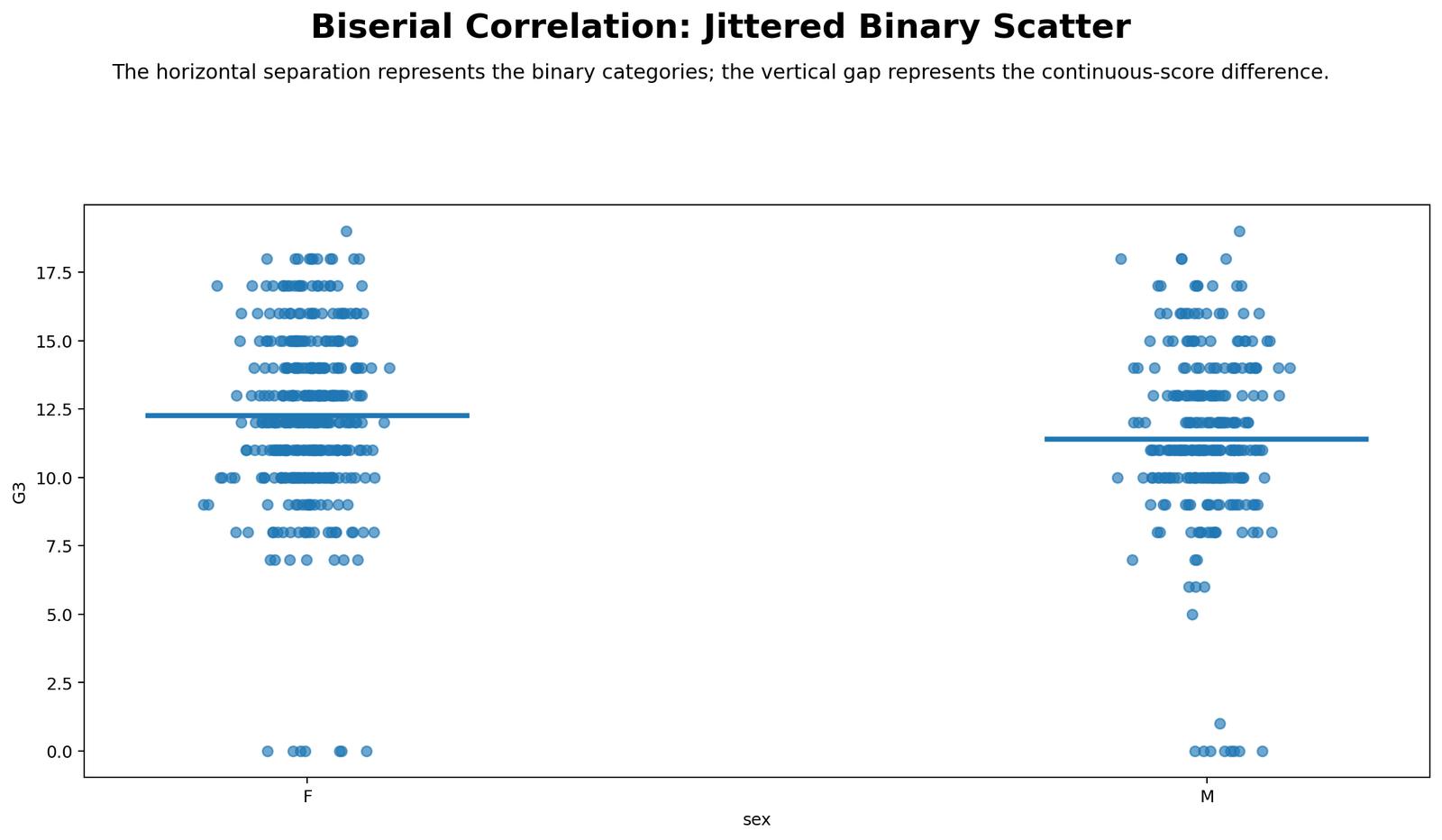
The jittered scatterplot displays the individual student scores instead of only summary boxes or means. The horizontal separation represents the binary groups, while the vertical position represents G3. The horizontal mean line is higher for F than for M, matching the mean chart. The individual dots show substantial overlap between groups, especially from about 8 to 16.
This chart prevents overinterpretation. The significant result does not mean every F-coded student scored higher than every M-coded student. Many students in both groups have similar grades. The association is driven by a small average shift and the presence of slightly more lower-end values in the M-coded group.
Python Chart 5: Statistical Summary Report Card
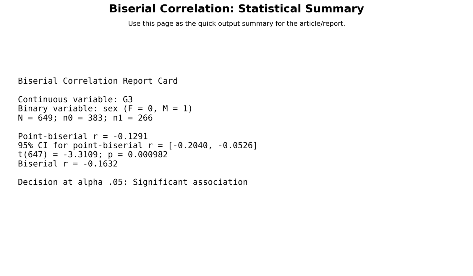
The report card gives the final output in one place: continuous variable G3, binary variable sex, N = 649, n0 = 383, n1 = 266, point-biserial r = -0.1291, 95% CI [-0.2040, -0.0526], t(647) = -3.3109, p = .000982, and biserial r = -0.1632. The decision line states that the association is significant at alpha .05.
This is the best chart to use when writing the final result paragraph. It contains the sample size, coding, coefficient, confidence interval, test statistic, p-value and decision. The interpretation should still mention that the effect is small, because statistical significance is strengthened by the large sample size.
R Chart-by-Chart Validation
The R charts validate the same result using a separate workflow. They repeat the distribution, mean, coefficient, scatter and report-card views with a colorful style. This software-to-software agreement supports the reliability of the reported values.
R Chart 1: Colorful Scores by Binary Group
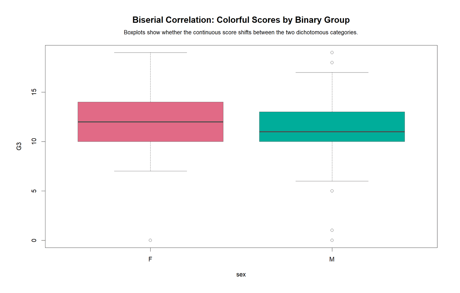
The R boxplot confirms the Python pattern. The F group has a slightly higher central line and a wider upper spread, while the M group has a lower center and multiple low outlying values. Both groups cover much of the same G3 range, so the practical separation is limited.
This visual agreement matters because it confirms that the small negative correlation is not a Python plotting artifact. The same group pattern appears when the analysis is recreated in R.
R Chart 2: Colorful Group Mean Difference
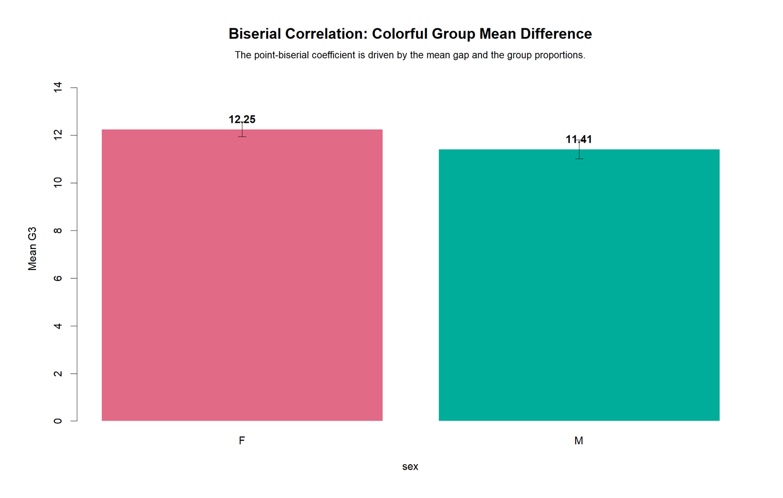
The R mean chart labels the same average values: approximately 12.25 for F and 11.41 for M. The bars make the direction easy to see, and the error bars show that the group means are estimated precisely in this large sample.
The correct report sentence should connect direction and coding. Since M is coded 1, the lower M mean produces a negative point-biserial coefficient. Reversing the coding would reverse the sign but not the strength.
R Chart 3: Colorful Coefficient Comparison
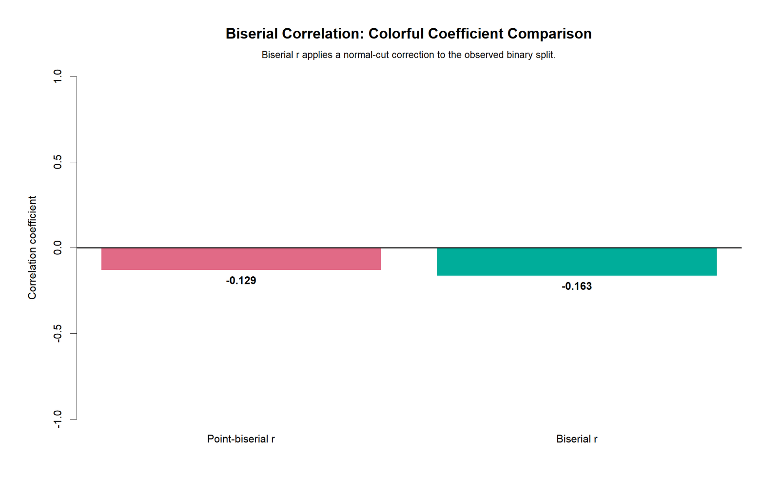
The R coefficient chart again shows point-biserial r = -0.129 and biserial r = -0.163. The larger absolute biserial estimate reflects the normal-cut adjustment. The values are both small in magnitude, so the result is statistically detectable but not practically large.
This chart is useful for teaching because it visually separates the observed coefficient from the corrected estimate. It also makes clear that the biserial correction does not change the direction of the association.
R Chart 4: Colorful Binary Scatter
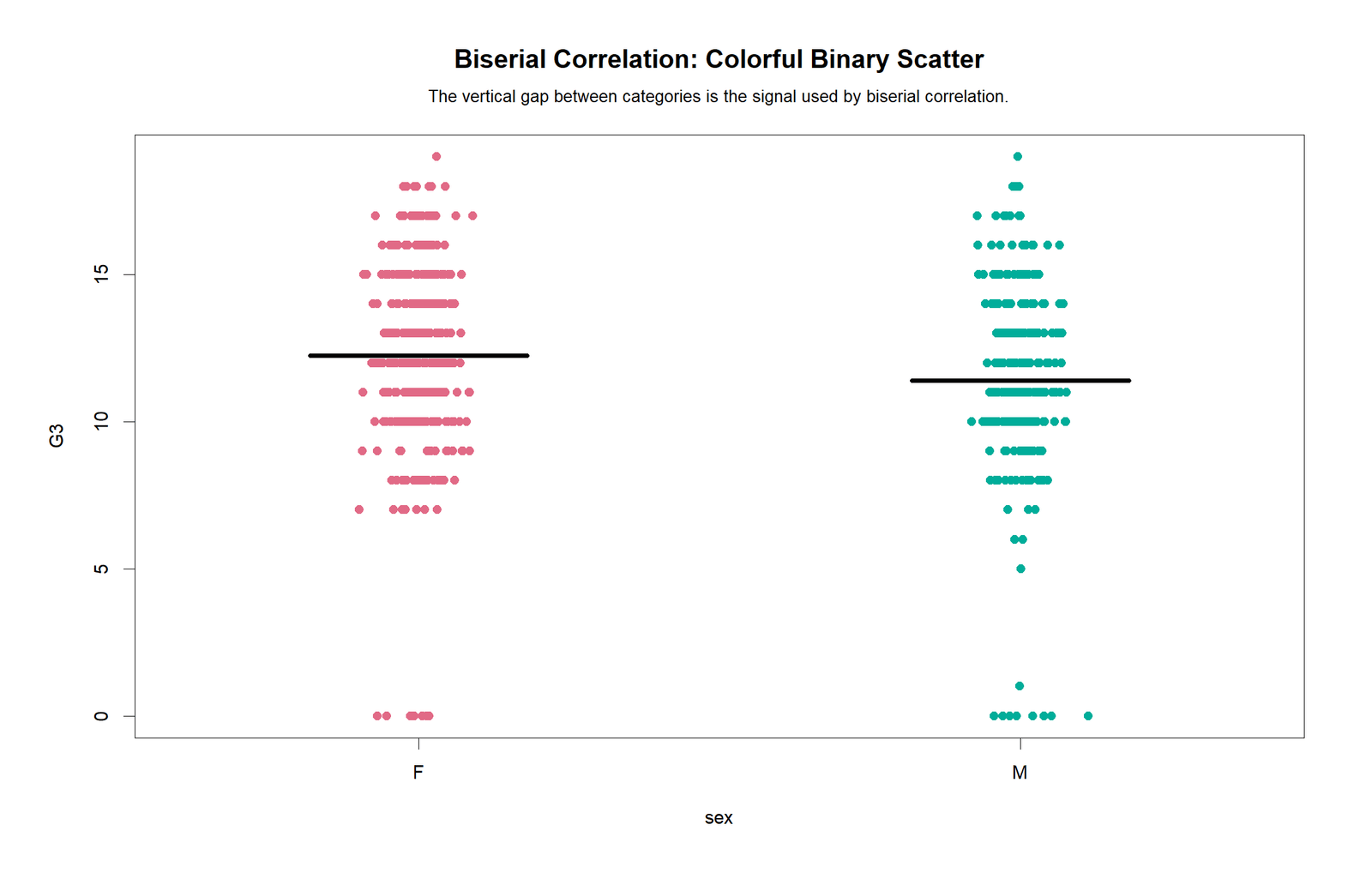
The R scatterplot shows two vertical clouds of observations. The F group and M group overlap heavily across the main score range, while the mean marker for F is above the mean marker for M. This is a small-shift pattern, not a strong-separation pattern.
The scatterplot is the most transparent visual because every observation is shown. It helps readers understand why a small coefficient can still be significant when the dataset is large.
R Chart 5: Colorful Statistical Summary
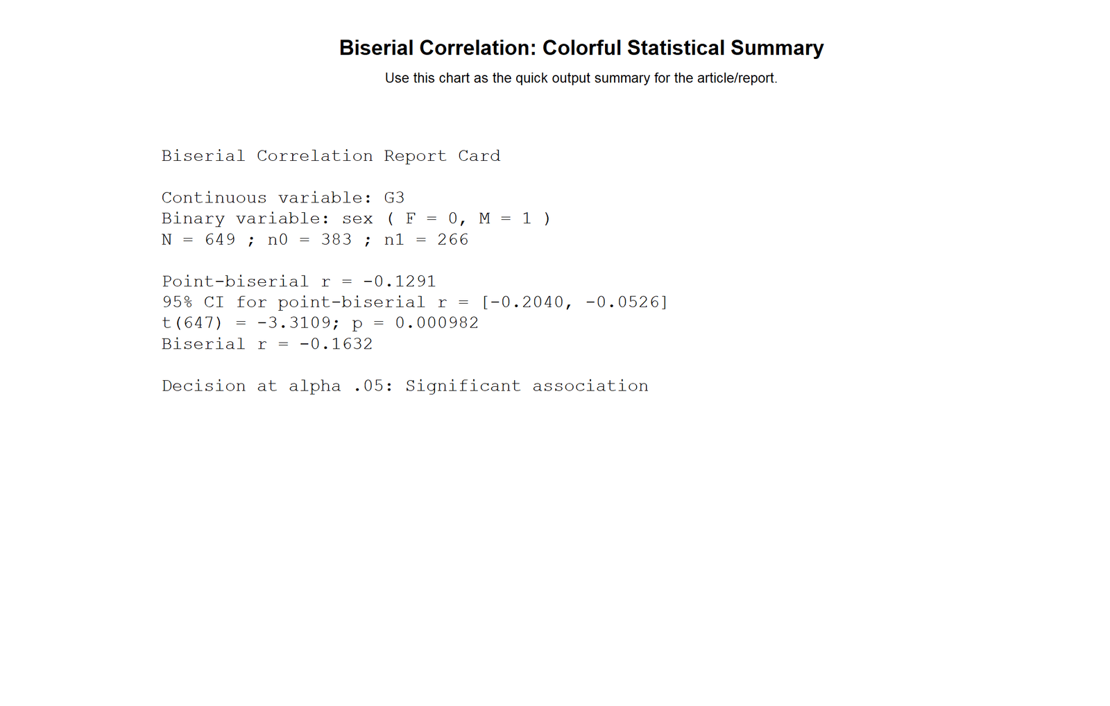
The R report card matches the Python report card: N = 649, n0 = 383, n1 = 266, point-biserial r = -0.1291, 95% CI [-0.2040, -0.0526], t(647) = -3.3109, p = .000982, and biserial r = -0.1632. This confirms the same final decision in R.
The final interpretation remains the same: the association is statistically significant, but the magnitude is small. The result should be reported with direction, coding, confidence interval and practical effect size language.
Excel Results Explained
The uploaded Excel workbook adds an important extra result. It does not only repeat the sex example. It also gives a fully worked formula-based example where G1 is artificially dichotomized using the rule G1 >= 10 and then compared with continuous G3. This is a stronger demonstration of true biserial correlation because G1 was originally a numeric grade variable before it was converted into two groups.
Excel Worked Example: G1 Dichotomized at 10 Against G3
| Excel Item | Value | Interpretation |
|---|---|---|
| Continuous outcome | G3 | Final grade is the continuous variable. |
| Dichotomized variable | G1 >= 10 | G1 was converted into low/fail and high/pass groups. |
| N | 649 | All valid paired observations were used. |
| n high/pass | 492 | About 75.8% of students were in the high/pass G1 group. |
| n low/fail | 157 | About 24.2% of students were in the low/fail G1 group. |
| Mean G3 in high/pass group | 13.0224 | Students with G1 >= 10 had much higher final grades. |
| Mean G3 in low/fail group | 8.4076 | Students with G1 below 10 had much lower final grades. |
| Mean difference | 4.6147 | The outcome gap is large in grade-score units. |
| SD of G3 | 3.2307 | This standard deviation is used in the coefficient formulas. |
| Point-biserial r | 0.6117 | Strong observed binary-continuous association. |
| Biserial r | 0.8390 | Very strong corrected estimate for the underlying continuous G1 trait. |
| t statistic | 19.6684 | Very large test statistic based on the point-biserial coefficient. |
| df | 647 | Degrees of freedom for the significance test. |
| p-value | 7.24 × 10-68 | The relationship is statistically significant at .05. |
This Excel result is much stronger than the sex example because the split variable is directly related to school performance. When G1 is converted into a high/pass versus low/fail group, the group means on G3 are far apart: 13.02 versus 8.41. The point-biserial coefficient of 0.6117 already shows a strong observed relationship, and the biserial correction increases the estimate to 0.8390 because the binary split is treated as a cut of an underlying continuous grade variable.
The workbook also calculates median-split biserial relationships for several numeric variables against G3. The strongest corrected biserial result is G2 with rb = 0.8841, followed by G1 with rb = 0.8281. Studytime is positive but smaller (rb = 0.2976). Mother’s education and father’s education are also positive and significant. Some lifestyle variables are negative, including weekend alcohol use (Walc, rb = -0.1405) and free time (freetime, rb = -0.1217). Age, absences, health and goout are not statistically significant in the workbook table.
Excel interpretation rule: The G1 >= 10 example is the better biserial example because the binary variable was created from a numeric variable. The sex example is better described as point-biserial correlation, with the biserial coefficient included only as a normal-cut comparison.
Excel Formula Steps Used in the Workbook
| Step | Excel Formula Pattern | Purpose |
|---|---|---|
| Count valid observations | =COUNT(Y_range) | Find N. |
| Count group 1 | =COUNTIF(binary_range,1) | Find n1. |
| Count group 0 | =COUNTIF(binary_range,0) | Find n0. |
| Calculate p and q | =n1/N and =n0/N | Find group proportions. |
| Calculate group means | =AVERAGEIF(binary_range,1,Y_range) | Find M1 and M0. |
| Calculate standard deviation | =STDEV.S(Y_range) | Find SD of the continuous outcome. |
| Find normal cutoff | =NORM.S.INV(q) | Find the z cutoff for the dichotomy. |
| Find normal ordinate | =NORM.S.DIST(z_cutoff,FALSE) | Find the height of the normal curve at the cutoff. |
| Point-biserial r | =((M1-M0)/SD_Y)*SQRT(p*q) | Observed binary-continuous correlation. |
| Biserial r | =((M1-M0)/SD_Y)*(p*q/y) | Normal-cut corrected estimate. |
SPSS, R, Python and Excel Workflows for Biserial Correlation
The same analysis can be reproduced in all four tools. The exact method depends on whether the binary variable is true binary or artificially dichotomized.
| Software | Main Steps | Best Use |
|---|---|---|
| SPSS | Recode the binary variable to 0/1, run Pearson correlation for point-biserial, run independent-samples t-test for mean difference context and calculate biserial manually if needed. | Formal output PDF, thesis reporting and classroom verification. |
| Python | Use pandas for coding, scipy for correlation and t-test, statsmodels or manual formulas for confidence intervals, and matplotlib for charts. | Automated chart production and reproducible reporting. |
| R | Use cor(), cor.test(), t.test(), group summaries and manual biserial formula. | Statistical validation and flexible publication charts. |
| Excel | Use COUNT, COUNTIF, AVERAGEIF, STDEV.S, NORM.S.INV, NORM.S.DIST, CORREL and T.DIST.2T formulas. | Step-by-step teaching and fully worked formula explanation. |
Code Blocks for Biserial Correlation
SPSS Syntax for Biserial Correlation
* Biserial / point-biserial correlation in SPSS.
* Continuous variable: G3.
* Binary variable: sex coded F = 0 and M = 1.

OUTPUT CLOSE ALL.
OUTPUT NEW NAME=Biserial_Output.

* Example assumes data are already open in SPSS.
RECODE sex ('F'=0) ('M'=1) INTO sex_binary.
VARIABLE LABELS sex_binary 'Binary variable coded 0/1 for point-biserial and biserial correlation'.
VALUE LABELS sex_binary 0 'F / group 0' 1 'M / group 1'.
EXECUTE.

FREQUENCIES VARIABLES=sex sex_binary.
DESCRIPTIVES VARIABLES=G3 sex_binary /STATISTICS=MEAN STDDEV MIN MAX.

CORRELATIONS
  /VARIABLES=G3 sex_binary
  /PRINT=TWOTAIL
  /MISSING=PAIRWISE.

T-TEST GROUPS=sex_binary(0 1)
  /VARIABLES=G3
  /CRITERIA=CI(.95).

EXAMINE VARIABLES=G3 BY sex_binary
  /PLOT BOXPLOT HISTOGRAM NPPLOT
  /STATISTICS DESCRIPTIVES
  /CINTERVAL 95
  /MISSING LISTWISE.

OUTPUT EXPORT
  /CONTENTS EXPORT=VISIBLE
  /PDF DOCUMENTFILE='Biserial-Correlation-SPSS-Output.pdf'.
Python Code for Biserial Correlation
import pandas as pd
import numpy as np
from scipy import stats

# Load data
df = pd.read_csv("dataset.csv")

# Continuous variable and binary coding
work = df[["sex", "G3"]].dropna().copy()
work["sex_binary"] = work["sex"].map({"F": 0, "M": 1})
work["G3"] = pd.to_numeric(work["G3"], errors="coerce")
work = work.dropna()

x = work["sex_binary"].to_numpy()
y = work["G3"].to_numpy()
n = len(work)

# Point-biserial correlation
r_pb, p_value = stats.pearsonr(x, y)
t_value = r_pb * np.sqrt((n - 2) / (1 - r_pb**2))
df_t = n - 2

# Group summaries
m0 = y[x == 0].mean()
m1 = y[x == 1].mean()
sd_y = y.std(ddof=1)
p = (x == 1).mean()
q = (x == 0).mean()
z_cutoff = stats.norm.ppf(q)
y_ordinate = stats.norm.pdf(z_cutoff)

# Biserial correlation
r_b = ((m1 - m0) / sd_y) * ((p * q) / y_ordinate)

# Fisher confidence interval for point-biserial r
z = np.arctanh(r_pb)
se = 1 / np.sqrt(n - 3)
ci_low, ci_high = np.tanh([z - 1.96 * se, z + 1.96 * se])

print("N:", n)
print("Mean group 0:", m0, "Mean group 1:", m1)
print("Point-biserial r:", r_pb)
print("95% CI:", ci_low, ci_high)
print("t:", t_value, "df:", df_t, "p:", p_value)
print("Biserial r:", r_b)
R Code for Biserial Correlation
# Biserial / point-biserial correlation in R

df <- read.csv("dataset.csv")
work <- na.omit(df[, c("sex", "G3")])
work$sex_binary <- ifelse(work$sex == "M", 1, 0)
work$G3 <- as.numeric(work$G3)

# Point-biserial correlation is Pearson correlation with 0/1 coding
cor_test <- cor.test(work$sex_binary, work$G3)
print(cor_test)

n <- nrow(work)
m0 <- mean(work$G3[work$sex_binary == 0])
m1 <- mean(work$G3[work$sex_binary == 1])
sd_y <- sd(work$G3)
p <- mean(work$sex_binary == 1)
q <- mean(work$sex_binary == 0)
z_cutoff <- qnorm(q)
y_ordinate <- dnorm(z_cutoff)

r_b <- ((m1 - m0) / sd_y) * ((p * q) / y_ordinate)
cat("Biserial r =", r_b, "\n")

# Mean difference context
t.test(G3 ~ sex_binary, data = work, var.equal = TRUE)
Excel Formulas for Biserial Correlation
Assume:
Y_range = continuous G3 values
binary_range = 0/1 group coding

N:
=COUNT(Y_range)

n1 and n0:
=COUNTIF(binary_range,1)
=COUNTIF(binary_range,0)

p and q:
=n1/N
=n0/N

Group means:
=AVERAGEIF(binary_range,1,Y_range)
=AVERAGEIF(binary_range,0,Y_range)

Standard deviation of Y:
=STDEV.S(Y_range)

Point-biserial r:
=((M1-M0)/SD_Y)*SQRT(p*q)

Normal cutoff and ordinate:
=NORM.S.INV(q)
=NORM.S.DIST(z_cutoff,FALSE)

Biserial r:
=((M1-M0)/SD_Y)*(p*q/y_ordinate)

Significance test based on point-biserial r:
=r_pb*SQRT((N-2)/(1-r_pb^2))
=T.DIST.2T(ABS(t),N-2)
APA Reporting Wording for Biserial Correlation
When reporting a Biserial Correlation or point-biserial correlation, describe the continuous variable, the binary coding, group counts, group means, coefficient, confidence interval, p-value, and whether the coefficient is an observed point-biserial result or a biserial normal-cut correction.
APA-Style Full Report
A point-biserial correlation was computed to examine the association between sex coding and G3 final grade. Sex was coded as F = 0 and M = 1. The analysis included 649 students, with 383 students in the F group and 266 students in the M group. The F group had a higher mean G3 score (M = 12.25) than the M group (M = 11.41). The point-biserial correlation was statistically significant and small, r = -.129, 95% CI [-.204, -.053], t(647) = -3.311, p = .001. The corresponding biserial normal-cut estimate was rb = -.163. Because the M group was coded as 1 and had the lower mean, the coefficient was negative.
Short APA-Style Version
A small but statistically significant point-biserial association was found between sex coding and G3, r = -.129, 95% CI [-.204, -.053], p = .001. The biserial corrected estimate was rb = -.163. The negative sign reflects the coding direction because M was coded as 1 and had a lower mean G3 score than F.
Excel Worked-Example Wording
For the Excel artificial-dichotomy example, G1 was converted to a binary variable using the cutoff G1 >= 10 and correlated with continuous G3. The high/pass group had a much higher mean G3 score (M = 13.02) than the low/fail group (M = 8.41). The point-biserial correlation was strong, r = .612, t(647) = 19.668, p < .001. The biserial corrected estimate was very strong, rb = .839, indicating that the underlying G1 performance trait was strongly related to final G3 performance.
Common Mistakes in Biserial Correlation Interpretation
| Mistake | Why It Is a Problem | Better Practice |
|---|---|---|
| Calling every 0/1 correlation “biserial” | True binary variables are usually point-biserial, not biserial. | Use point-biserial for true binary variables and biserial for artificial dichotomies. |
| Ignoring coding direction | The sign depends on which group is coded 1. | Always report the coding, such as F = 0 and M = 1. |
| Reporting only p-value | A large sample can make small effects significant. | Report r, CI, p-value and practical effect size language. |
| Using biserial correction without explaining the cutoff | The correction depends on the normal cutoff and group proportions. | State the cutoff rule and why it represents an artificial dichotomy. |
| Confusing rank-biserial with point-biserial | Rank-biserial belongs to nonparametric/rank-based comparisons. | Use rank-biserial for rank-based group comparisons and point-biserial for raw 0/1 continuous correlation. |
| Assuming significance means strong association | The main report is significant but small. | Describe the result as statistically significant but small when r is near .10 to .20. |
When to Use Biserial Correlation
Use biserial correlation when one variable is continuous and the other variable is binary because it was created by cutting a continuous or latent variable into two groups. Examples include pass/fail from an exam score, high/low anxiety from a scale score, or high/low performance from a continuous grade.
Use point-biserial correlation when the binary variable is naturally binary. Examples include treatment/control, yes/no, present/absent, group 0/group 1 or sex coded as 0/1. Use rank-biserial correlation when the analysis is rank-based or tied to a Mann-Whitney style comparison. If both variables are continuous, use ordinary Pearson correlation instead.
Downloads and Resources for Biserial Correlation
R Biserial Correlation Report PDFIncludes R validation charts for the same binary-continuous workflow.
SPSS Biserial Correlation Output PDFSPSS output file for group counts, descriptives, t-test context and manual biserial calculation.
Excel Fully Worked FileExcel workbook with formulas, dashboard, G1 dichotomy worked example and multiple biserial results.
FAQs About Biserial Correlation
What is biserial correlation in simple words?
Biserial correlation estimates the relationship between a continuous variable and a binary variable that was created by splitting an underlying continuous variable into two groups.
What is point-biserial correlation?
Point-biserial correlation is the Pearson correlation between a true 0/1 binary variable and a continuous variable.
What is the difference between biserial and point-biserial correlation?
Point-biserial correlation is used for true binary variables. Biserial correlation is used when the binary variable is an artificial dichotomy from an underlying continuous or latent trait.
How do I interpret point-biserial correlation?
Interpret it like Pearson r, but remember that the sign depends on which binary group is coded 1. A positive r means the group coded 1 has a higher mean on the continuous variable; a negative r means the group coded 1 has a lower mean.
How do I calculate point-biserial correlation in Excel?
Code the binary variable as 0 and 1, then use CORREL(binary_range, continuous_range). You can also use the mean-difference formula with group means, standard deviation and group proportions.
How do I calculate biserial correlation in Excel?
Calculate group means, the continuous-variable standard deviation, group proportions p and q, the normal cutoff with NORM.S.INV(q), the normal ordinate with NORM.S.DIST(z,FALSE), and then use r_b = ((M1-M0)/SD_Y)*(p*q/y).
How do I run point-biserial correlation in SPSS?
Recode the binary variable to 0/1, then run Pearson correlation between the 0/1 variable and the continuous variable. Add an independent-samples t-test for group mean context.
Is point-biserial correlation parametric?
Point-biserial correlation is a parametric correlation related to Pearson correlation and the independent-samples t-test. It is commonly used when the continuous variable is reasonably measured and the groups are independent.
Can ordinal data be used in point-biserial correlation?
If the outcome is truly ordinal or rank-based, rank-biserial correlation or another nonparametric effect size may be more appropriate. Point-biserial works best with a continuous outcome.
Why is the biserial coefficient larger than the point-biserial coefficient?
The biserial coefficient applies a normal-cut correction. It estimates the relationship before the continuous or latent variable was dichotomized, so its magnitude can be larger than the observed point-biserial correlation.

