
2×2 contingency table, binary association, chi-square connection and effect-size interpretation
Phi Coefficient: Formula, Interpretation, SPSS, Python, R and Excel Guide
Phi Coefficient, written as φ, is a correlation-style effect-size measure for the association between two binary variables. It is most commonly used with a 2×2 contingency table, such as sex by pass/fail status, treatment by success/failure, exposed by disease/no disease, or yes/no by yes/no. This guide explains the formula, the chi-square relationship, Python charts, R validation charts, SPSS output, Excel worked formulas, expected counts, standardized residuals, odds ratio, risk ratio, APA reporting and common mistakes.
Quick Answer: Phi Coefficient Result
The worked example in this report tests the association between sex and Pass_Status. The outcome variable is created from G3 final grade, where Pass = G3 ≥ 10 and Fail = G3 < 10. The predictor has two categories: Female and Male. Because both variables are binary, the correct effect-size measure for the 2×2 table is the Phi Coefficient.
The verified Excel calculation gives φ = 0.078222, χ²(1) = 3.971035, and p = 0.046289. At α = .05, the result is statistically significant. However, the effect size is very small. The practical conclusion is that sex and pass/fail status are associated in this sample, but the strength of association is negligible to small.
Final interpretation: The 2×2 table shows a statistically significant association between sex and pass/fail status, but the Phi Coefficient is only 0.078. This means the observed association is very weak in practical terms. The result should not be written as a strong difference between groups.
Important distinction: The p-value answers whether the association is statistically detectable. The Phi Coefficient answers how strong the association is. Here, the p-value is below .05, but the Phi value is close to zero, so the practical strength remains very small.
Table of Contents
- What Is the Phi Coefficient?
- When Should You Use Phi Coefficient?
- Phi Coefficient Formula
- Null and Alternative Hypotheses
- Dataset and Variables Used
- 2×2 Contingency Table
- Verified Phi Coefficient Results
- Expected Counts and Standardized Residuals
- Python Chart-by-Chart Interpretation
- R Chart-by-Chart Interpretation
- SPSS Output Interpretation
- Excel Worked File Explanation
- Python, R, SPSS and Excel Workflows
- Code Blocks and Excel Formulas
- Assumptions and Data Checks
- How to Report Phi Coefficient
- Common Mistakes
- Downloads and Resources
- Related Statistical Guides
- FAQs About Phi Coefficient
What Is the Phi Coefficient?
Phi Coefficient is a measure of association between two binary variables. A binary variable has only two categories, such as pass/fail, yes/no, male/female, treatment/control, exposed/not exposed, present/absent, success/failure, or correct/incorrect. When both variables have two categories, the data can be arranged in a 2×2 contingency table, and Phi Coefficient provides a signed effect-size measure for the association.
Phi behaves like a correlation coefficient. It can be positive, negative, or near zero depending on the arrangement of the 2×2 table. A positive value means the table has more weight along one diagonal. A negative value means the table has more weight along the opposite diagonal. A value near zero means the observed table is close to what would be expected under independence.
The Phi Coefficient is closely connected to the chi-square test of independence. For a 2×2 table, the relationship is:
This means that if you know the sample size and Phi, you can calculate the chi-square statistic. In this worked example, n = 649 and φ = 0.078222, so χ² = 649 × 0.078222² = 3.971035. That value gives the p-value of 0.046289 with 1 degree of freedom.
Phi Coefficient connects naturally with Cross Tabulation, Contingency Coefficient, Correlation Matrix, Correlation Assumptions, p-value, Effect Size, Confidence Interval, Null and Alternative Hypothesis and Parametric vs Nonparametric Tests.
Simple definition: Phi Coefficient measures the strength and direction of association between two binary variables in a 2×2 contingency table.
When Should You Use Phi Coefficient?
Use the Phi Coefficient when both variables are binary and the data form a 2×2 table. It is especially useful when you need a compact effect size to accompany a chi-square test. The chi-square test tells whether the variables are independent; Phi tells how strong the association is.
| Situation | Use Phi? | Reason | Example |
|---|---|---|---|
| Both variables have exactly two categories | Yes | Phi is designed for 2×2 tables. | sex by pass/fail status |
| One variable is binary and the other is binary outcome | Yes | The table has four observed cells. | treatment/control by success/failure |
| You already ran chi-square for a 2×2 table | Yes | Phi provides the effect-size interpretation. | χ² test plus φ |
| One variable has more than two categories | No, not directly | Use Cramer’s V or another association measure. | school type by grade category with 3+ levels |
| Both variables are continuous | No | Use Pearson, Spearman or Kendall correlation depending on assumptions. | G1 by G3 grades |
| One variable is binary and the other is continuous | No | Use point-biserial correlation or a t-test. | sex by G3 numeric score |
For this example, sex has two categories and Pass_Status has two categories. Therefore, the 2×2 table is appropriate for Phi. If the outcome were the full numeric G3 score, Phi would not be the correct measure; a biserial or point-biserial correlation, t-test in Python, t-test in R, or t-test in SPSS would be more suitable.
Phi Coefficient Formula
For a 2×2 table, label the four cells as follows:
| Outcome Positive | Outcome Negative | Row Total | |
|---|---|---|---|
| Group 1 | a | b | a + b |
| Group 2 | c | d | c + d |
| Column Total | a + c | b + d | n |
The signed Phi Coefficient formula is:
The numerator ad − bc compares the diagonal products of the table. If ad is larger than bc, Phi is positive. If bc is larger than ad, Phi is negative. If the two diagonal products are similar, Phi is near zero.
| Formula Element | Meaning | Value in This Example |
|---|---|---|
| a | Female + Pass | 333 |
| b | Female + Fail | 50 |
| c | Male + Pass | 216 |
| d | Male + Fail | 50 |
| ad | 333 × 50 | 16,650 |
| bc | 50 × 216 | 10,800 |
| ad − bc | Net diagonal difference | 5,850 |
| Denominator | √[(383)(266)(549)(100)] | 74,787.045670 |
| Phi | φ | 0.078222 |
The positive sign appears because the diagonal product a × d is larger than b × c. In plain language, the observed pattern is slightly more concentrated in the Female-Pass and Male-Fail diagonal than the opposite diagonal. However, the size of the coefficient is still very small.
Null and Alternative Hypotheses
The Phi Coefficient is usually reported with the chi-square test of independence. The hypotheses are about whether the two binary variables are independent in the population.
| Statement | Hypothesis | Meaning |
|---|---|---|
| Null hypothesis | H0: φ = 0 | Sex and pass/fail status are independent; there is no binary association. |
| Alternative hypothesis | H1: φ ≠ 0 | Sex and pass/fail status are associated. |
| Decision rule | Reject H0 if p < .05 | The association is statistically significant at the 5% level. |
| Observed decision | p = 0.046289 | Reject H0, but interpret effect size as negligible. |
Decision: Since p = 0.046289 is below .05, the null hypothesis of independence is rejected. The variables are statistically associated, but the effect size is very small because φ = 0.078222.
Dataset and Variables Used
The analysis uses the student performance dataset with 649 valid cases. The predictor is sex, coded as Female and Male. The outcome is Pass_Status, created from G3 final grade. A student is classified as Pass if G3 is at least 10 and Fail if G3 is below 10.
| Variable | Role | Categories | Reason Used |
|---|---|---|---|
| sex | Binary predictor | Female, Male | Creates the two rows of the 2×2 table. |
| G3 | Original grade variable | 0 to 19 observed grade scores | Used to create the pass/fail outcome. |
| Pass_Status | Binary outcome | Pass, Fail | Creates the two columns of the 2×2 table. |
| Pass rule | Outcome coding rule | Pass = G3 ≥ 10; Fail = G3 < 10 | Converts numeric G3 into a binary outcome for Phi. |
This conversion is important. Phi is not used on the original numeric G3 score. It is used only after G3 is converted into a binary outcome. If the research question requires keeping G3 as a numeric score, then the correct method would be a different analysis, such as Biserial Correlation, Two Sample t-Test, t-Test in Excel or t-Test in Python.
2×2 Contingency Table
The 2×2 table below is the core of the Phi Coefficient calculation. Rows represent sex, and columns represent pass/fail status. The table has four observed cells and row/column totals.
| sex \ Pass_Status | Pass (G3 ≥ 10) | Fail (G3 < 10) | Row Total | Pass % Within Row | Fail % Within Row |
|---|---|---|---|---|---|
| Female | 333 | 50 | 383 | 86.95% | 13.05% |
| Male | 216 | 50 | 266 | 81.20% | 18.80% |
| Column Total | 549 | 100 | 649 | 84.59% overall pass | 15.41% overall fail |
The table shows that 86.95% of female students passed, compared with 81.20% of male students. The difference in pass proportions is 5.74 percentage points. This difference is enough to produce a statistically significant chi-square result at the .05 level, but it is not large enough to produce a strong effect size.
The risk ratio is 1.0707, meaning the pass proportion for female students is about 1.07 times the pass proportion for male students. The odds ratio is 1.5417, meaning the odds of passing are higher in the female group than the male group under this coding. However, because the Phi value is only 0.0782, all of these results should be described carefully as small or negligible in association strength.
Verified Phi Coefficient Results
The main calculation is shown below. This section is useful for students who need the exact values for interpretation, reporting, and checking formulas in Excel, Python, R, or SPSS.
| Statistic | Value | Interpretation |
|---|---|---|
| Female + Pass | 333 | Count in row 1 column 1. |
| Female + Fail | 50 | Count in row 1 column 2. |
| Male + Pass | 216 | Count in row 2 column 1. |
| Male + Fail | 50 | Count in row 2 column 2. |
| Total N | 649 | Total valid cases in the 2×2 table. |
| Phi coefficient | 0.078222 | Positive but negligible binary association. |
| Chi-square statistic | 3.971035 | Test statistic for independence. |
| Degrees of freedom | 1 | A 2×2 table has df = 1. |
| p-value | 0.046289 | Statistically significant at α = .05. |
| Cramer’s V | 0.078222 | Same magnitude as |Phi| for a 2×2 table. |
| Odds ratio | 1.541667 | Female pass odds divided by male pass odds. |
| Risk Female Pass | 0.869452 | Female pass proportion. |
| Risk Male Pass | 0.812030 | Male pass proportion. |
| Risk difference | 0.057422 | Female pass proportion minus male pass proportion. |
| Risk ratio | 1.070714 | Female pass proportion divided by male pass proportion. |
| Effect-size label | Negligible | The relationship is statistically significant but very weak. |
The most important result is not only the p-value. The p-value tells whether the observed table differs enough from independence to be statistically detectable. The Phi Coefficient tells whether that difference is practically meaningful. Here, the result is statistically significant but very small.
Expected Counts and Standardized Residuals
Expected counts show what the table would look like if sex and pass/fail status were independent. Residuals show how far the observed counts are from those expected counts. Standardized residuals make the cell differences easier to compare across the table.
| Cell | Predictor Level | Outcome Level | Observed | Expected | Residual | Standardized Residual | Chi-square Contribution |
|---|---|---|---|---|---|---|---|
| a | Female | Pass | 333 | 323.9861 | 9.0139 | 0.5008 | 0.2508 |
| b | Female | Fail | 50 | 59.0139 | -9.0139 | -1.1734 | 1.3768 |
| c | Male | Pass | 216 | 225.0139 | -9.0139 | -0.6009 | 0.3611 |
| d | Male | Fail | 50 | 40.9861 | 9.0139 | 1.4080 | 1.9824 |
| Total | 649 | 649 | 0 | 3.9710 |
The largest standardized residual is in the Male + Fail cell, with a standardized residual of about 1.408. This means male failures are somewhat higher than expected under independence. The Female + Fail cell is lower than expected, and the Female + Pass cell is higher than expected. These cell-level patterns explain why Phi is positive under the selected table mapping.
Even so, the standardized residuals are not extremely large. This supports the same conclusion as the Phi value: there is a detectable association, but the pattern is not strong.
Python Chart-by-Chart Interpretation
The Python report includes five visuals: the 2×2 contingency heatmap, row percentages, observed versus expected counts, standardized residuals, and effect-size summary. Together, these charts explain the full Phi Coefficient result from raw counts to final interpretation.
Python Chart 1: 2×2 Contingency Heatmap
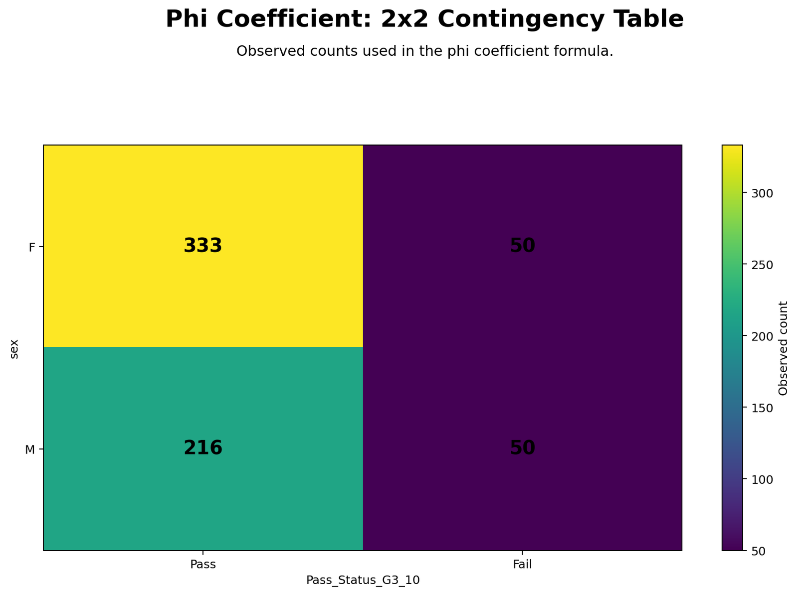
This heatmap displays the four observed counts: Female-Pass = 333, Female-Fail = 50, Male-Pass = 216, and Male-Fail = 50. It gives the simplest visual summary of the 2×2 table. The largest cell is Female-Pass because the female group has more students and most students passed overall.
The chart should be interpreted with row totals in mind. Female has 383 cases and Male has 266 cases, so raw counts alone can be misleading if read without percentages. That is why the row-percentage chart is also required. The heatmap tells where the counts are located; the percentage chart tells how the outcome rate differs within each group.
Python Chart 2: Row Percentages
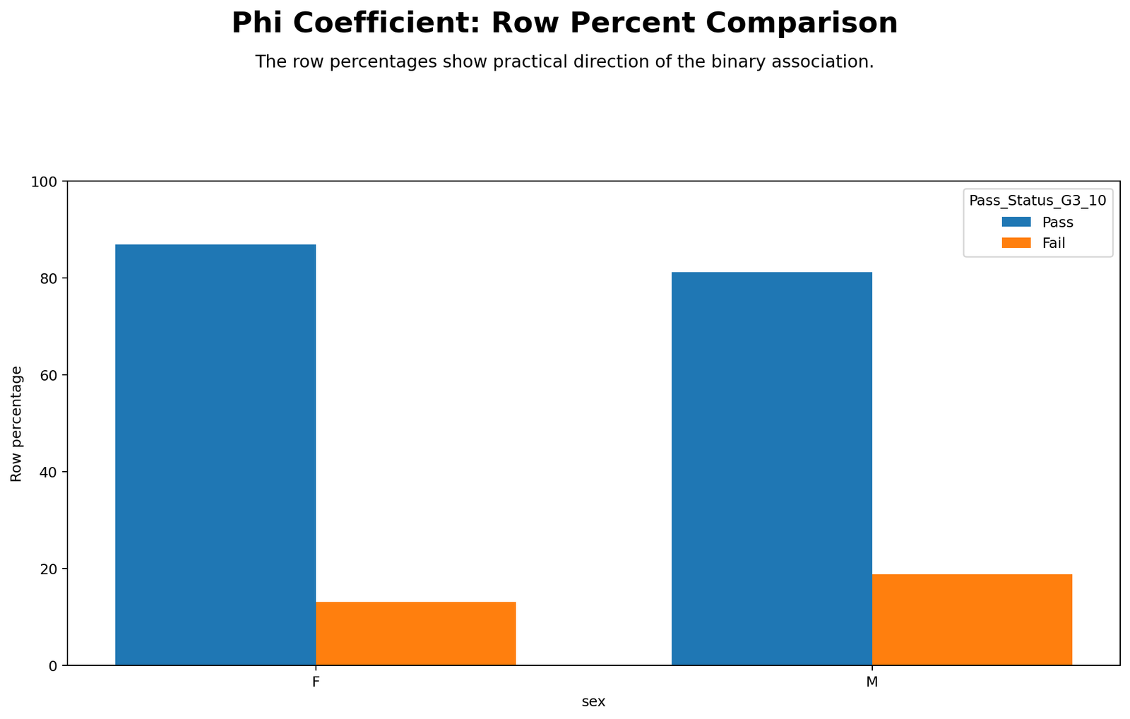
The row-percentage chart shows the practical group comparison. Female students have a pass percentage of about 86.95%, while male students have a pass percentage of about 81.20%. The fail percentages are about 13.05% for female students and 18.80% for male students.
This chart explains the direction of the association. The female group has a higher pass percentage and a lower fail percentage than the male group. However, the percentage difference is only about 5.74 percentage points. This is why the association is statistically significant but practically small.
Python Chart 3: Observed vs Expected Counts
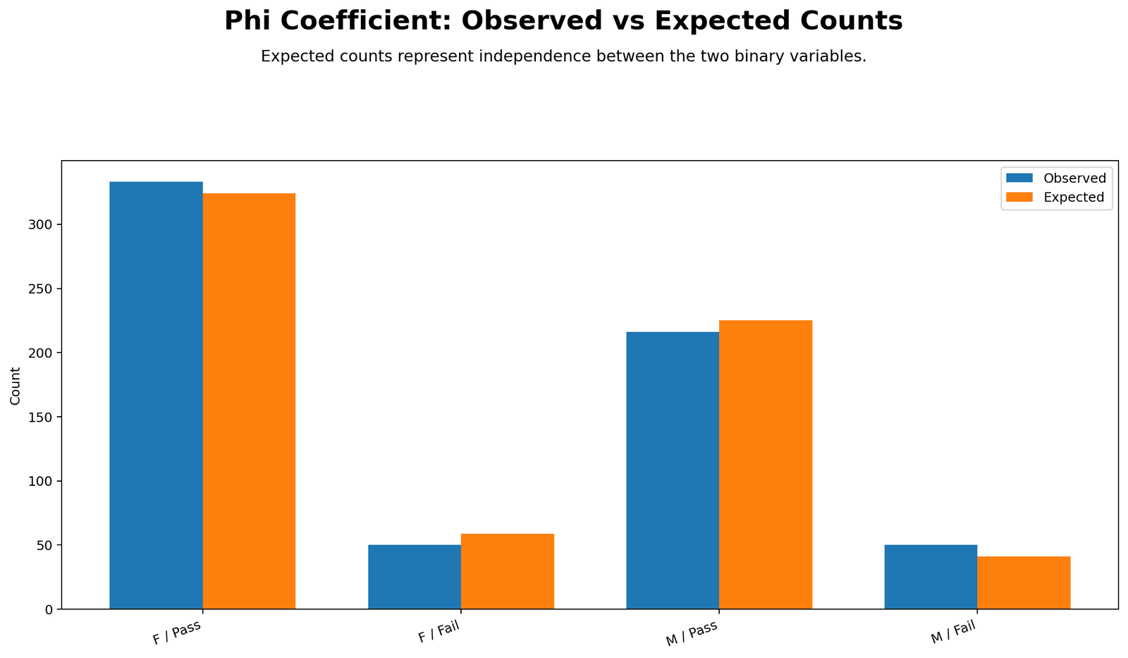
The observed-versus-expected chart compares each actual cell count with the count expected if sex and pass/fail status were independent. Female-Pass is observed at 333 and expected at about 323.99. Female-Fail is observed at 50 and expected at about 59.01. Male-Pass is observed at 216 and expected at about 225.01. Male-Fail is observed at 50 and expected at about 40.99.
The differences are consistent with a positive Phi value: more Female-Pass and Male-Fail cases than expected, and fewer Female-Fail and Male-Pass cases than expected. However, the observed counts are not extremely far from the expected counts, which supports the negligible effect-size interpretation.
Python Chart 4: Standardized Residuals
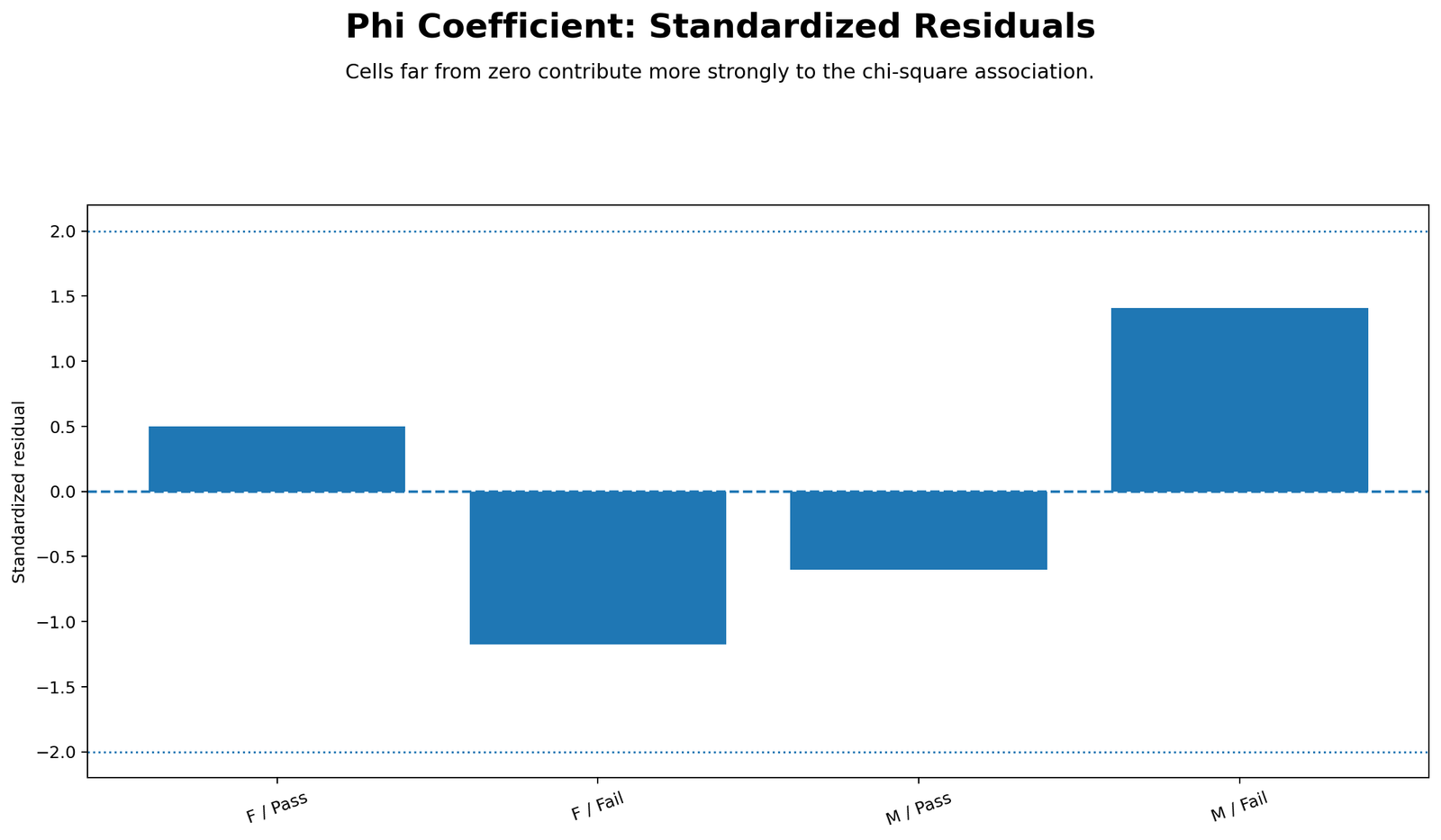
The standardized residual chart shows which cells contribute most to the chi-square statistic. The Male-Fail cell has the largest positive standardized residual, around 1.408. The Female-Fail cell has a negative standardized residual around -1.173. The Female-Pass and Male-Pass cells have smaller residuals.
This chart is important because the p-value alone does not show where the association comes from. The residuals show that the association is mainly driven by somewhat fewer Female-Fail cases than expected and somewhat more Male-Fail cases than expected. Still, the residual values are not large enough to suggest a strong cell-level departure.
Python Chart 5: Phi Effect Size Summary
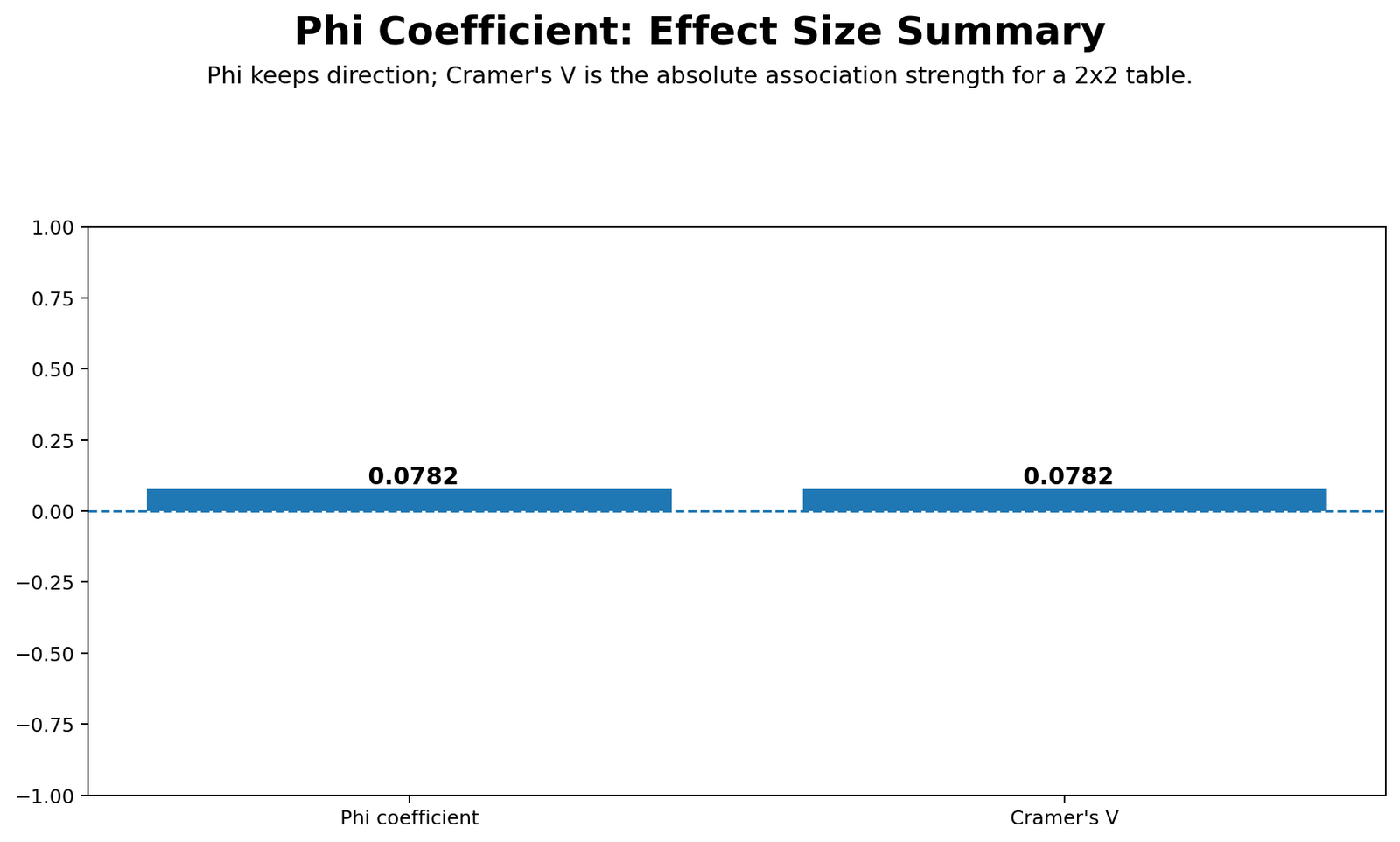
The effect-size summary chart gives the final report values in one place: Phi = 0.078222, chi-square = 3.971035, p = 0.046289, odds ratio = 1.541667, risk ratio = 1.070714, and risk difference = 0.057422. This chart is the best visual to use when writing the final interpretation paragraph.
The key reporting lesson is that statistical significance and effect size must be separated. The p-value is just below .05, so the result is statistically significant. But Phi is below .10, so the association is negligible or very small in practical strength.
R Chart-by-Chart Interpretation
The R report validates the Python result using a separate workflow and colorful visuals. The same five chart types are repeated: 2×2 contingency heatmap, row percentages, observed versus expected counts, standardized residuals and effect-size summary.
R Chart 1: Colorful 2×2 Contingency Heatmap
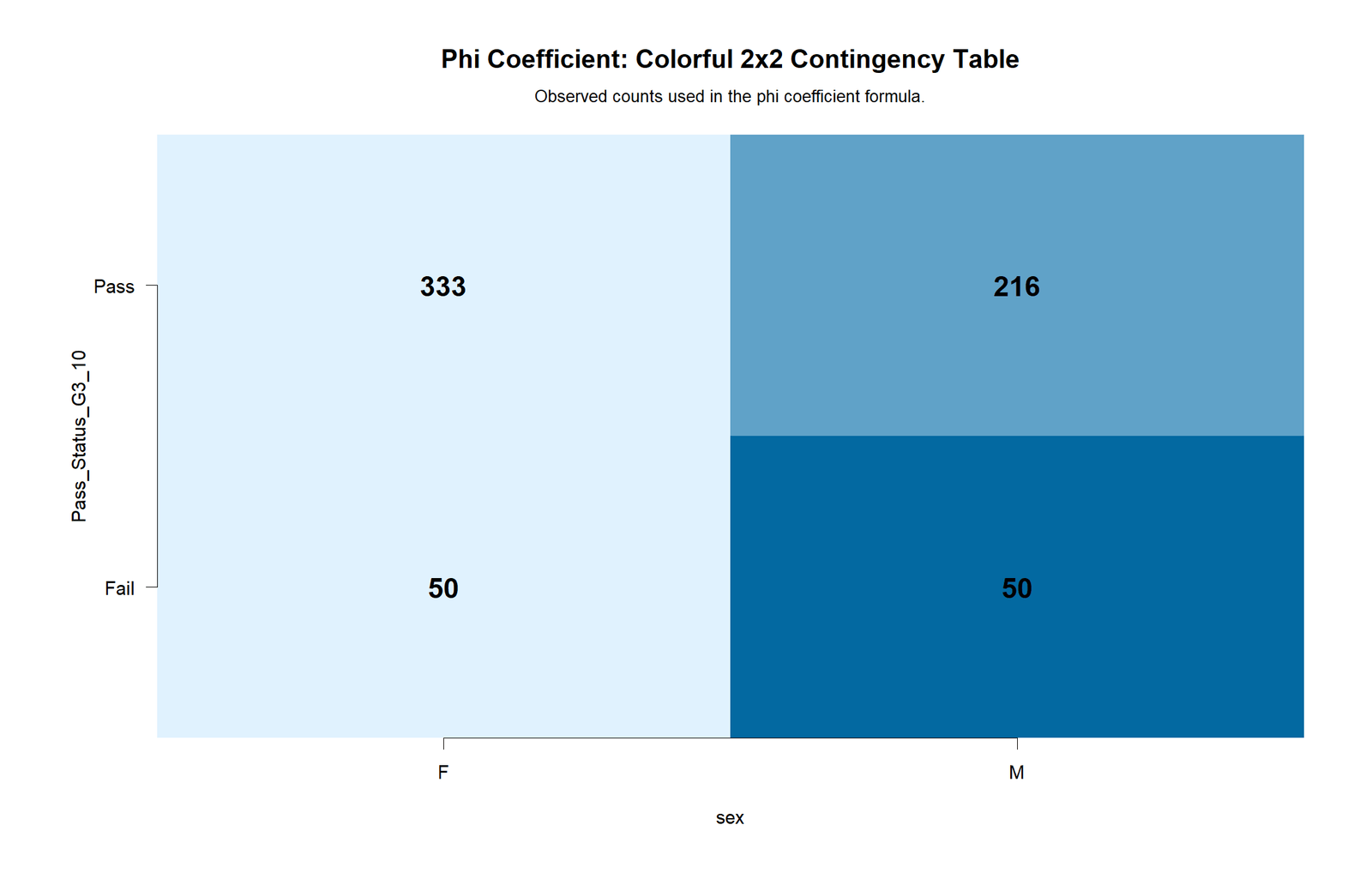
The R contingency heatmap confirms the same observed 2×2 structure. Female-Pass is the largest cell, Female-Fail and Male-Fail are equal at 50, and Male-Pass is 216. This confirms that the R workflow is using the same binary coding and the same table as the Python and Excel workflows.
R Chart 2: Colorful Row Percentages
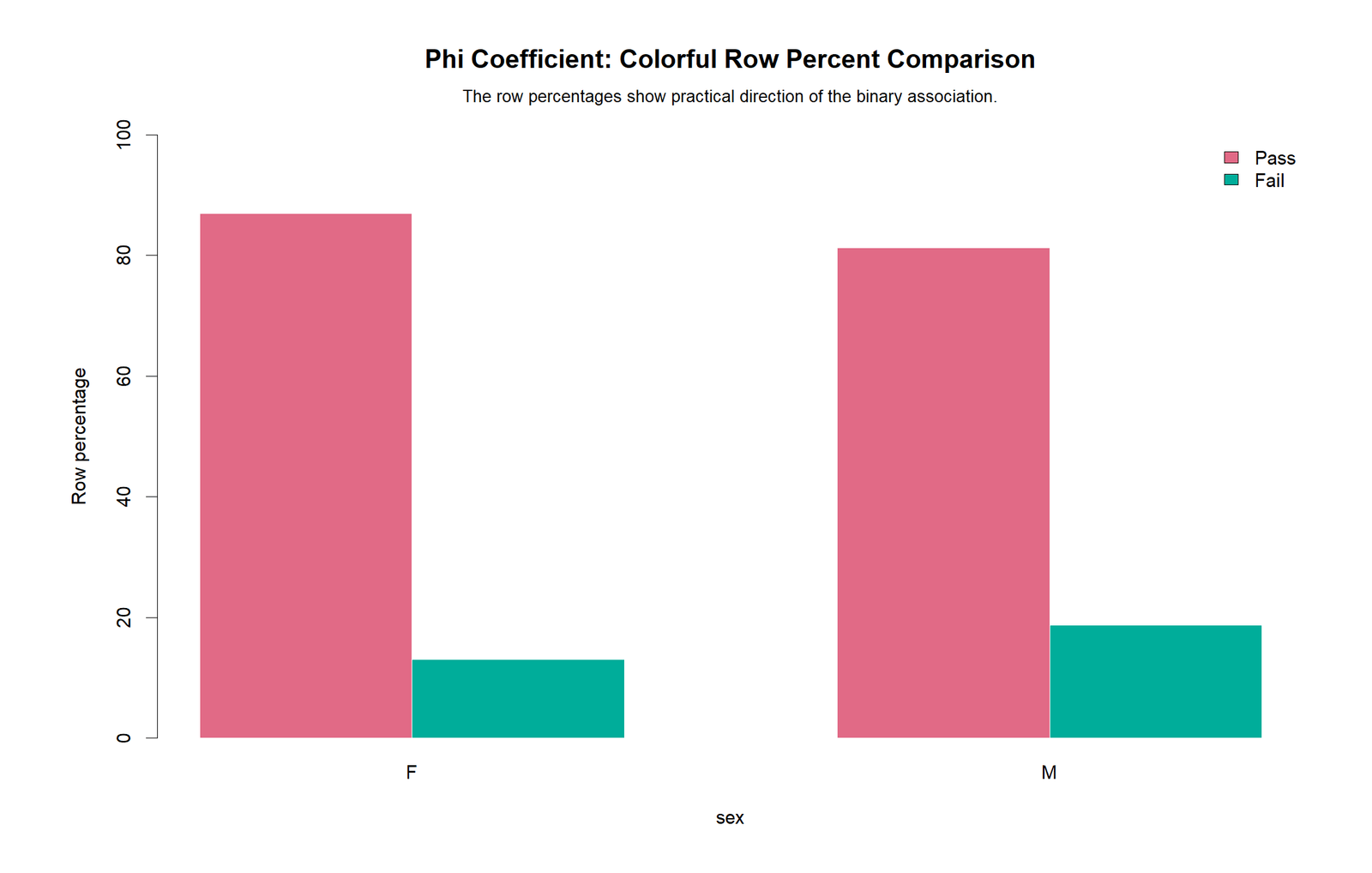
The R row-percentage chart confirms that the female group has a higher pass percentage and the male group has a higher fail percentage. The difference is visible, but not large. This is exactly the pattern that produces a significant p-value with a small Phi effect size.
R Chart 3: Colorful Observed vs Expected Counts
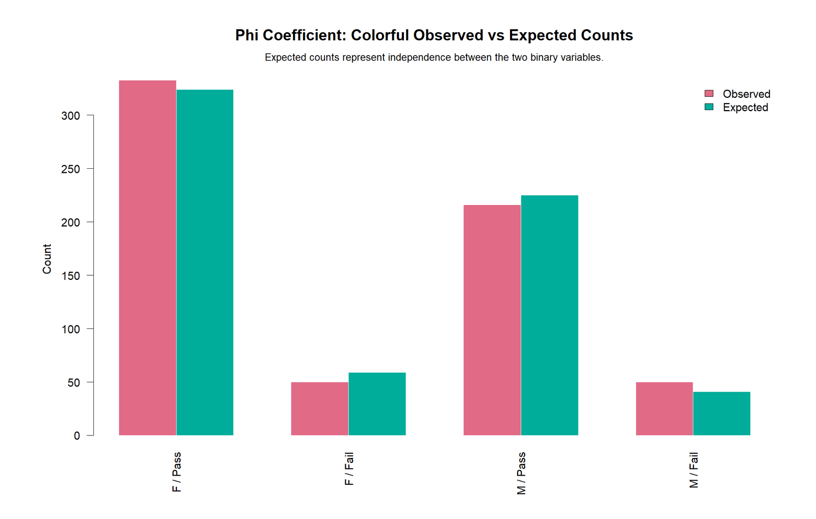
The R observed-versus-expected chart validates the same expected-count pattern. Female-Pass and Male-Fail are higher than expected, while Female-Fail and Male-Pass are lower than expected. The departures are enough to reject independence at the .05 level, but they remain modest in size.
R Chart 4: Colorful Standardized Residuals
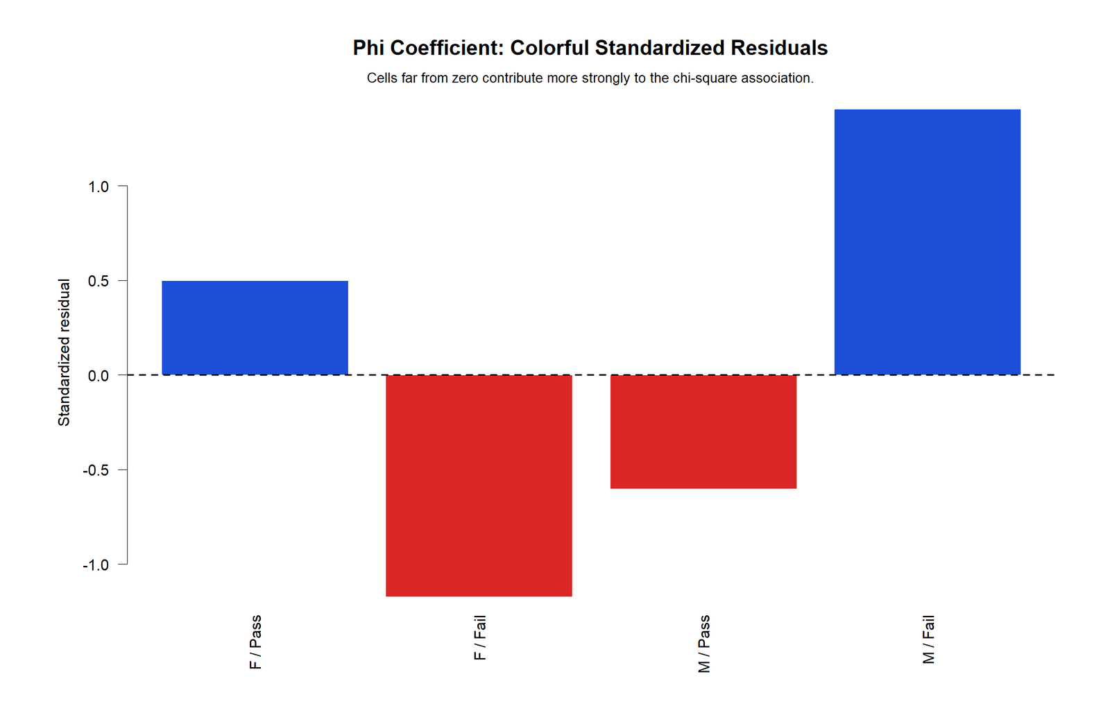
The R residual chart confirms that the largest cell-level departure is the Male-Fail cell. This cell has more cases than expected under independence. The Female-Fail cell has fewer cases than expected. These two cells explain much of the chi-square contribution.
R Chart 5: Colorful Phi Effect Size Summary
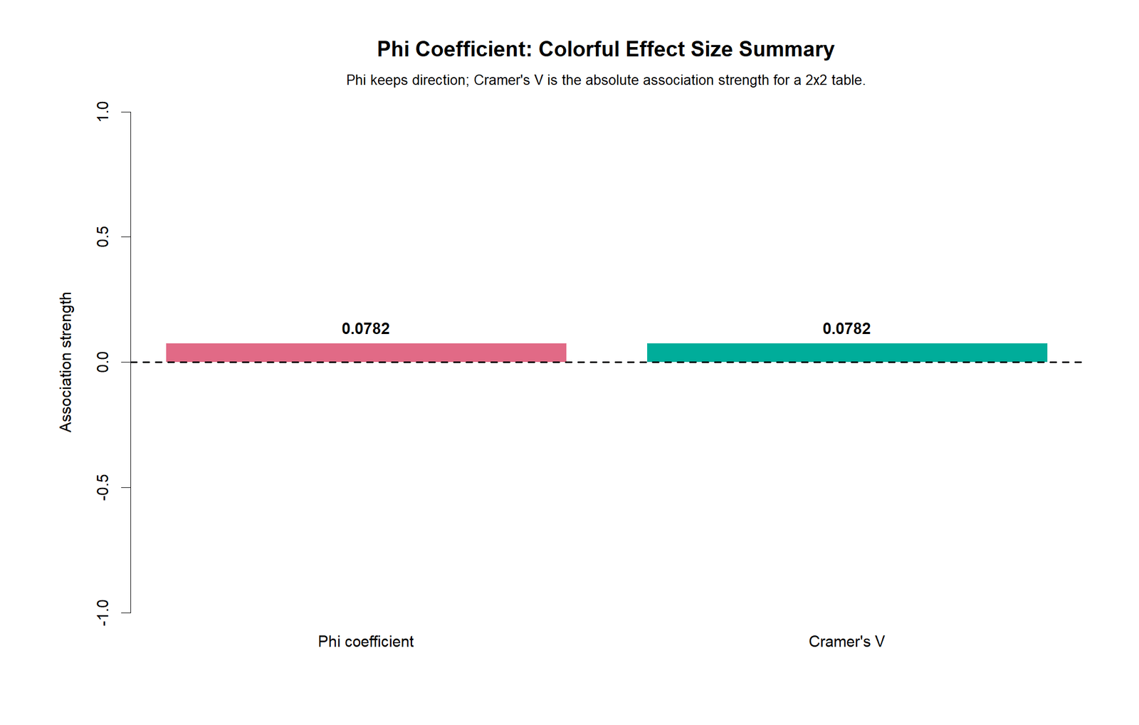
The R effect-size summary confirms the same final conclusion. Phi is positive and statistically significant, but it is very small. The correct final wording is a statistically significant but negligible association, not a strong relationship.
SPSS Output Interpretation
The SPSS output PDF is included as the formal software output for the 2×2 table. In SPSS, Phi is usually reported in the Symmetric Measures table after running Crosstabs with Chi-square statistics selected. The Pearson chi-square table gives the test of independence, while the Phi and Cramer’s V row gives the effect-size magnitude.
| SPSS Output Item | Expected Value | How to Interpret It |
|---|---|---|
| Crosstabulation | Female/Male by Pass/Fail | Shows the observed 2×2 table. |
| Pearson Chi-square | χ² = 3.971 | Tests whether sex and pass status are independent. |
| df | 1 | A 2×2 table has one degree of freedom. |
| Asymptotic significance | p = .046 | Statistically significant at α = .05. |
| Phi | φ = .078 | Negligible/small effect size. |
| Cramer’s V | V = .078 | Same magnitude as Phi for a 2×2 table. |
| N of valid cases | 649 | Total sample used in the table. |
In a thesis or research report, the SPSS result should not be interpreted only from the chi-square significance row. The Phi row is necessary because it gives the strength of association. Here, the association is statistically significant but weak enough that the practical conclusion should remain cautious.
Excel Worked File Explanation
The Excel workbook provides a full formula-based Phi Coefficient analysis. It contains the dataset, binary coding, contingency table, full worked Phi calculation, expected counts, standardized residuals and chart source tables. This makes the file useful for students who want to understand each calculation step rather than relying only on SPSS, Python or R output.
Download the Phi Coefficient Full Excel Analysis File
| Excel Sheet | Purpose | What It Teaches |
|---|---|---|
| README | Summarizes the analysis. | Shows the test, folder, dataset, variables, hypotheses and main result. |
| Dataset | Stores the original uploaded data. | Allows the user to verify all raw variables. |
| Binary_Coding | Creates binary variables. | Shows how sex and pass/fail status were coded for the 2×2 table. |
| Contingency_Table | Builds the observed 2×2 table. | Uses COUNTIFS formulas to count Female/Male by Pass/Fail. |
| Phi_Calculation | Shows the formula step by step. | Calculates denominator, Phi, chi-square, p-value, Cramer’s V, odds ratio, risk difference and risk ratio. |
| Expected_Residuals | Compares observed and expected counts. | Shows residuals, standardized residuals and chi-square contributions. |
| Chart_Data | Stores chart source tables. | Feeds the 2×2 heatmap, row percentage chart and summary visuals. |
Excel Main Calculation
The workbook calculates the denominator as 74,787.045670. The Phi formula then gives φ = 0.0782221031. The chi-square value is calculated as n × φ², giving 3.9710346255. The p-value is calculated using Excel’s right-tail chi-square function and equals 0.0462893224.
Excel Risk and Odds Measures
The workbook also adds practical 2×2 table measures. The female pass proportion is 0.869452, and the male pass proportion is 0.812030. The risk difference is 0.057422, and the risk ratio is 1.070714. The odds ratio is 1.541667. These measures give useful context, but the overall association strength is still summarized by the small Phi value.
Excel teaching value: The workbook is not only a result file. It shows the entire chain from binary coding to contingency table, formula calculation, expected counts, residuals, chi-square, p-value and effect-size interpretation.
Python, R, SPSS and Excel Workflows
The same Phi Coefficient analysis can be reproduced in Python, R, SPSS and Excel. The workflow is always the same: create two binary variables, build the 2×2 table, calculate Phi, run chi-square, inspect expected counts and interpret the effect size.
| Software | Main Workflow | Best Use |
|---|---|---|
| Python | Use pandas for coding and crosstab, scipy for chi-square, and manual formulas for Phi, odds ratio and risk measures. | Automated charts, reports, heatmaps and reproducible analysis. |
| R | Use table(), chisq.test(), manual Phi formula and charting functions for validation visuals. | Independent validation and colorful statistical charts. |
| SPSS | Use Crosstabs with Chi-square and Phi/Cramer’s V under Statistics. | Formal output for assignments, theses and institutional reports. |
| Excel | Use COUNTIFS, SQRT, CHISQ.DIST.RT, expected-count formulas and residual calculations. | Transparent formula-based learning and teaching. |
Code Blocks and Excel Formulas
Python Code for Phi Coefficient
import pandas as pd
import numpy as np
from scipy.stats import chi2_contingency, chi2

# Load data
df = pd.read_csv("dataset.csv")

# Create binary outcome
df["Pass_Status"] = np.where(df["G3"] >= 10, "Pass", "Fail")

# Build 2x2 table: rows = sex, columns = pass/fail status
table = pd.crosstab(df["sex"], df["Pass_Status"])
table = table.loc[["F", "M"], ["Pass", "Fail"]]

# Extract cell counts
a = table.loc["F", "Pass"]
b = table.loc["F", "Fail"]
c = table.loc["M", "Pass"]
d = table.loc["M", "Fail"]

# Phi coefficient
denominator = np.sqrt((a+b) * (c+d) * (a+c) * (b+d))
phi = ((a*d) - (b*c)) / denominator

# Chi-square relationship
n = table.to_numpy().sum()
chi_square_from_phi = n * phi**2
p_value = chi2.sf(chi_square_from_phi, df=1)

# Chi-square test using scipy for expected counts
chi2_stat, chi2_p, dof, expected = chi2_contingency(table, correction=False)

# Practical measures
risk_female = a / (a + b)
risk_male = c / (c + d)
risk_difference = risk_female - risk_male
risk_ratio = risk_female / risk_male
odds_ratio = (a * d) / (b * c)

print("2x2 table:")
print(table)
print("Phi:", phi)
print("Chi-square:", chi_square_from_phi)
print("p-value:", p_value)
print("Expected counts:")
print(expected)
print("Risk difference:", risk_difference)
print("Risk ratio:", risk_ratio)
print("Odds ratio:", odds_ratio)
R Code for Phi Coefficient
df <- read.csv("dataset.csv", stringsAsFactors = FALSE)

# Create binary pass/fail outcome
df$Pass_Status <- ifelse(df$G3 >= 10, "Pass", "Fail")

# Build 2x2 table
tab <- table(df$sex, df$Pass_Status)
tab <- tab[c("F", "M"), c("Pass", "Fail")]

# Extract cells
a <- tab["F", "Pass"]
b <- tab["F", "Fail"]
c <- tab["M", "Pass"]
d <- tab["M", "Fail"]

# Phi coefficient
denominator <- sqrt((a+b) * (c+d) * (a+c) * (b+d))
phi <- ((a*d) - (b*c)) / denominator

# Chi-square relationship
n <- sum(tab)
chi_square <- n * phi^2
p_value <- pchisq(chi_square, df = 1, lower.tail = FALSE)

# Chi-square test
chi_result <- chisq.test(tab, correct = FALSE)

# Practical measures
risk_female <- a / (a + b)
risk_male <- c / (c + d)
risk_difference <- risk_female - risk_male
risk_ratio <- risk_female / risk_male
odds_ratio <- (a * d) / (b * c)

print(tab)
cat("Phi =", phi, "\n")
cat("Chi-square =", chi_square, "\n")
cat("p-value =", p_value, "\n")
cat("Risk difference =", risk_difference, "\n")
cat("Risk ratio =", risk_ratio, "\n")
cat("Odds ratio =", odds_ratio, "\n")
print(chi_result)
SPSS Syntax for Phi Coefficient
* Phi Coefficient in SPSS.
* Predictor: sex.
* Outcome: Pass_Status from G3 where Pass = G3 >= 10.

OUTPUT CLOSE ALL.
OUTPUT NEW NAME=Phi_Coefficient_Output.

* Example assumes dataset is already open in SPSS.
RECODE G3 (Lowest thru 9=0) (10 thru Highest=1) INTO pass_status.
VARIABLE LABELS pass_status 'Pass status from G3: 1=Pass, 0=Fail'.
VALUE LABELS pass_status 0 'Fail (G3 < 10)' 1 'Pass (G3 >= 10)'.
EXECUTE.

CROSSTABS
  /TABLES=sex BY pass_status
  /FORMAT=AVALUE TABLES
  /STATISTICS=CHISQ PHI
  /CELLS=COUNT EXPECTED ROW COLUMN RESID SRESID
  /COUNT ROUND CELL.

OUTPUT EXPORT
  /CONTENTS EXPORT=VISIBLE
  /PDF DOCUMENTFILE='Phi-Coefficient-SPSS-Output.pdf'.
Excel Formulas for Phi Coefficient
Assume the 2x2 table is:

            Pass    Fail
Female       a       b
Male         c       d

Female + Pass:
=COUNTIFS(sex_range,"F",pass_status_range,"Pass")

Female + Fail:
=COUNTIFS(sex_range,"F",pass_status_range,"Fail")

Male + Pass:
=COUNTIFS(sex_range,"M",pass_status_range,"Pass")

Male + Fail:
=COUNTIFS(sex_range,"M",pass_status_range,"Fail")

Denominator:
=SQRT((a+b)*(c+d)*(a+c)*(b+d))

Phi:
=((a*d)-(b*c))/SQRT((a+b)*(c+d)*(a+c)*(b+d))

Chi-square:
=N*Phi^2

p-value:
=CHISQ.DIST.RT(chi_square,1)

Expected count for each cell:
=(row_total*column_total)/grand_total

Residual:
=Observed-Expected

Standardized residual:
=(Observed-Expected)/SQRT(Expected)

Odds ratio:
=(a*d)/(b*c)

Risk in Female group:
=a/(a+b)

Risk in Male group:
=c/(c+d)

Risk difference:
=Risk_Female-Risk_Male

Risk ratio:
=Risk_Female/Risk_Male
Assumptions and Data Checks
Phi Coefficient is simple to calculate, but it still has important requirements. The most important requirement is that both variables must be binary. The observations should also be independent, and expected counts should be checked when using the chi-square p-value.
| Check | Why It Matters | Status in This Example |
|---|---|---|
| Two binary variables | Phi is designed for a 2x2 table. | sex has two groups and Pass_Status has two groups. |
| Independent observations | Each student should contribute only one row. | The dataset treats each row as one student. |
| Expected counts | Very small expected counts can affect chi-square accuracy. | Expected counts are all above 40, so chi-square is acceptable. |
| Clear coding | The sign of Phi depends on cell arrangement. | Rows and columns are explicitly labeled. |
| Effect size reported | A significant p-value does not show strength. | Phi = 0.078222 is reported and interpreted as negligible. |
| No causal claim | Association does not prove cause and effect. | The result is reported as association only. |
The expected-count check is especially strong here because the smallest expected cell count is about 40.99. This means the chi-square approximation is not threatened by tiny expected frequencies. The main caution is not the p-value calculation; it is interpretation. A statistically significant result with Phi below .10 should still be described as very weak.
How to Report Phi Coefficient
A good Phi Coefficient report should include the variables, sample size, 2x2 table result, chi-square statistic, degrees of freedom, p-value, Phi value, direction, and practical interpretation. If the table is meaningful for applied interpretation, also include row percentages, odds ratio, risk difference or risk ratio.
APA-style report: A chi-square test of independence was conducted to examine the association between sex and pass/fail status based on G3 final grade. The 2x2 table included 649 valid cases. The association was statistically significant, χ²(1, N = 649) = 3.971, p = .046. The Phi Coefficient was φ = .078, indicating a negligible positive association. Female students had a pass rate of 86.95%, compared with 81.20% for male students.
Short reporting version: Sex and pass/fail status were statistically associated, χ²(1, N = 649) = 3.971, p = .046, φ = .078. Although significant, the effect size was negligible, so the practical relationship was very weak.
Plain-language interpretation: The pass rate was slightly higher for female students than male students, but the overall binary association was very small. The data provide evidence of a detectable relationship, not a strong practical difference.
Common Mistakes in Phi Coefficient Interpretation
| Mistake | Why It Is a Problem | Better Practice |
|---|---|---|
| Using Phi for tables larger than 2x2 | Phi is designed for two binary variables. | Use Cramer's V for larger contingency tables. |
| Reporting only chi-square | Chi-square significance does not show effect size. | Report Phi with chi-square and p-value. |
| Calling φ = .078 a strong effect | The coefficient is close to zero. | Call it negligible or very weak. |
| Ignoring row percentages | Raw counts are affected by group sizes. | Compare percentages within rows. |
| Misreading the sign | The sign depends on the row and column coding. | State the coding and explain direction in words. |
| Claiming causation | Phi shows association, not cause and effect. | Use association wording unless the design supports causal inference. |
| Confusing Phi with point-biserial correlation | Point-biserial is for one binary and one continuous variable. | Use Phi only when both variables are binary. |
Downloads and Resources
Download R Report PDFR validation report with colorful Phi Coefficient charts.
Download Excel Worked FileFull formula-based Phi Coefficient workbook with 2x2 table, p-value and residuals.
Open Python 2x2 HeatmapObserved cell-count heatmap for sex by pass status.
Open R Effect SummaryColorful summary chart with Phi, chi-square, p-value and practical measures.
External References
For additional learning, review documentation and references on chi-square tests of independence, 2x2 contingency tables, Phi Coefficient, Cramer's V, odds ratios, risk ratios and standardized residuals. These concepts are commonly taught together because they describe different parts of the same binary association problem.
FAQs About Phi Coefficient
What is the Phi Coefficient?
Phi Coefficient is an effect-size measure for the association between two binary variables in a 2x2 contingency table.
What was the Phi Coefficient result in this guide?
The result was φ = 0.078222, χ²(1) = 3.971035, p = 0.046289, N = 649. The association was statistically significant but negligible in practical strength.
What variables were used?
The predictor was sex, and the outcome was Pass_Status, created from G3 final grade using the rule Pass = G3 ≥ 10 and Fail = G3 < 10.
Is Phi the same as Cramer's V?
For a 2x2 table, the magnitude of Cramer's V is the same as the absolute value of Phi. Phi can be signed depending on category coding, while Cramer's V is commonly reported as a nonnegative magnitude.
How is Phi related to chi-square?
For a 2x2 table, χ² = nφ². In this example, 649 × 0.078222² = 3.971035.
Can I use Phi for a 3x2 or 4x4 table?
No. Phi is mainly for 2x2 tables. For larger contingency tables, use Cramer's V, contingency coefficient or another appropriate categorical association measure.
Why is the result significant if Phi is so small?
The sample size is 649, so even a small departure from independence can become statistically significant. The p-value shows evidence against independence, while Phi shows the association is practically weak.
How should I report the result?
You can write: “Sex and pass/fail status were statistically associated, χ²(1, N = 649) = 3.971, p = .046, φ = .078. The effect size was negligible.”
Does Phi prove that sex causes pass or fail status?
No. Phi is an association measure. It does not prove causation. The result should be interpreted as a small association between the two binary variables.

