
ANOVA Post Hoc Test, Control Group Comparisons, Adjusted p-values and Confidence Intervals
Dunnett’s Test: Formula, Interpretation, SPSS, Python, R and Excel Guide
Dunnett’s Test is a post hoc multiple-comparison method used when every treatment group must be compared with one selected control group. Instead of comparing every pair of groups, Dunnett’s Test focuses on treatment-versus-control questions. In this worked Salar Cafe example, studytime group 1 is the control group, and groups 2, 3 and 4 are compared against it for G3 final grade.
Quick Answer: Dunnett’s Test Result
The Dunnett’s Test result shows that all three comparison groups are significantly higher than the control group. The control group is studytime group 1, with a mean G3 of about 10.84. Group 2 has a mean of about 12.09, group 3 has a mean of about 13.23, and group 4 has a mean of about 13.06.
The adjusted p-value chart shows that every treatment-versus-control comparison is below α = .05. The adjusted p-values are approximately 2.794e-05 for group 2 vs control, 2.422e-09 for group 3 vs control, and 0.0003436 for group 4 vs control. The confidence-interval chart also supports the same conclusion because the intervals for all treatment-control mean differences remain above zero.
Final interpretation: Dunnett’s Test indicates that studytime groups 2, 3 and 4 all have significantly higher G3 final-grade means than the control group, studytime group 1. The strongest treatment-control difference is group 3 versus control, followed by group 4 versus control and group 2 versus control.
Important reporting point: Dunnett’s Test is not designed to compare all pairs. It compares each treatment group with the selected control group. Therefore, this output should not be used to claim whether group 3 differs from group 4 or whether group 2 differs from group 4.
Table of Contents
- What Is Dunnett’s Test?
- Dunnett’s Test Formula
- Dunnett’s Test Hypotheses
- Dataset and Variables Used
- Dunnett Comparison Decision Summary
- Assumptions Before Dunnett’s Test
- SPSS Output Interpretation
- Python Chart-by-Chart Interpretation
- R Chart-by-Chart Validation
- SPSS, R, Python and Excel Workflows
- Code Blocks for Dunnett’s Test
- APA Reporting Wording
- Common Mistakes
- When to Use Dunnett’s Test
- Downloads and Resources
- Related Guides
- FAQs
What Is Dunnett’s Test?
Dunnett’s Test is a multiple-comparison procedure used after ANOVA when the research design has one control group and several treatment groups. It adjusts for multiple testing while keeping the analysis focused on the control comparison question.
This makes Dunnett’s Test different from all-pairs post hoc methods. A method such as Tukey, Bonferroni or Duncan may compare every possible pair, but Dunnett’s Test compares only each treatment group against the selected control. This is useful when the research question is not “which groups differ from each other?” but “which treatment groups differ from the control?”
In this example, studytime group 1 is treated as the control group. Groups 2, 3 and 4 are compared with group 1. The result shows that all three groups are significantly higher than the control group in mean G3 final grade.
Simple definition: Dunnett’s Test is an ANOVA post hoc test for comparing several treatment groups against one control group while adjusting the p-values and confidence intervals for multiple comparisons.
This guide connects naturally with One Way ANOVA, ANOVA in SPSS, ANOVA in R, ANOVA in Python, ANOVA Assumptions, P Value, Confidence Interval, Effect Size, Eta Squared and Omega Squared.
Dunnett’s Test Formula
Dunnett’s Test begins with the difference between each treatment mean and the selected control mean:
The standard error for each treatment-control difference is commonly based on the ANOVA mean square error and the sample sizes:
The test statistic is:
Dunnett’s method then adjusts the decision for the fact that several treatment groups are being compared with the same control group. Software usually reports adjusted p-values and adjusted confidence intervals. A comparison is significant when the adjusted p-value is below the selected alpha level, usually .05, or when the adjusted confidence interval does not include zero.
Key Terms in the Formula
| Symbol / Term | Meaning | Interpretation |
|---|---|---|
| X̄j | Treatment group mean | Mean G3 for studytime group 2, 3 or 4. |
| X̄control | Control group mean | Mean G3 for studytime group 1. |
| Dj | Mean difference | Treatment mean minus control mean. |
| MSE | Mean square error | Within-group error from ANOVA. |
| SE(Dj) | Standard error | Uncertainty in the treatment-control difference. |
| Adjusted p-value | Multiple-comparison p-value | Decision value after Dunnett adjustment. |
| Adjusted CI | Dunnett confidence interval | Significant if the interval does not cross zero. |
Practical rule: If the adjusted confidence interval for treatment minus control stays above zero, the treatment group has a significantly higher mean than the control group. If it crosses zero, the treatment is not clearly different from the control.
Dunnett’s Test Hypotheses
Dunnett’s Test uses one comparison for each treatment group against the control. In this example, group 1 is the control, so the hypotheses compare groups 2, 3 and 4 against group 1.
| Comparison | Null Hypothesis | Alternative Hypothesis | Dunnett Decision |
|---|---|---|---|
| Group 2 vs Control 1 | μ2 = μ1 | μ2 ≠ μ1 | Significant; group 2 is higher than control. |
| Group 3 vs Control 1 | μ3 = μ1 | μ3 ≠ μ1 | Significant; group 3 is higher than control. |
| Group 4 vs Control 1 | μ4 = μ1 | μ4 ≠ μ1 | Significant; group 4 is higher than control. |
Decision for this example: Reject the control-equality null hypothesis for groups 2, 3 and 4. All three groups have significantly higher mean G3 than studytime group 1 after Dunnett adjustment.
Dataset and Variables Used
The worked example uses student performance data. The dependent variable is G3 final grade. The grouping factor is studytime, which has four groups. For Dunnett’s Test, studytime group 1 is selected as the control group.
| Variable | Role | Levels / Type | Why It Matters |
|---|---|---|---|
| G3 | Dependent variable | Numeric final grade | The outcome whose mean is compared against the control group. |
| studytime | Grouping factor | 1, 2, 3, 4 | Defines the control and treatment groups. |
| studytime 1 | Control group | Reference category | All other groups are compared against this group. |
Group Mean Pattern
| Studytime Group | Role | Approx. N | Mean G3 | Mean Difference vs Control | Interpretation |
|---|---|---|---|---|---|
| 1 | Control | 212 | 10.84 | Reference | Baseline group for all Dunnett comparisons. |
| 2 | Treatment / comparison | 305 | 12.09 | +1.25 | Significantly higher than control. |
| 3 | Treatment / comparison | 97 | 13.23 | +2.38 | Significantly higher than control and strongest difference. |
| 4 | Treatment / comparison | 35 | 13.06 | +2.21 | Significantly higher than control. |
The mean pattern explains the Dunnett result. Every comparison group is above the control mean. Group 3 has the largest observed difference from control, while group 4 is also far above control but has the smallest sample size.
For supporting concepts, review Descriptive Statistics, Mean Median and Mode, Standard Deviation, Variance, Standard Error, Confidence Interval, Five Number Summary, Box Plot Interpretation and Histogram Interpretation.
Dunnett Comparison Decision Summary
The Dunnett comparison table focuses only on treatment-control comparisons. It does not include all possible group pairs because that is not the purpose of Dunnett’s Test.
| Comparison | Mean Difference | Adjusted p-value | Adjusted CI Pattern | Decision | Interpretation |
|---|---|---|---|---|---|
| Group 2 − Control 1 | About +1.25 | 2.794e-05 | Above zero | Significant | Group 2 has higher mean G3 than control. |
| Group 3 − Control 1 | About +2.38 | 2.422e-09 | Above zero | Significant | Group 3 has higher mean G3 than control. |
| Group 4 − Control 1 | About +2.21 | 0.0003436 | Above zero | Significant | Group 4 has higher mean G3 than control. |
Best reporting summary: Dunnett’s Test showed that studytime groups 2, 3 and 4 each had significantly higher mean G3 than the control group, studytime group 1.
Assumptions Before Dunnett’s Test
Dunnett’s Test is usually interpreted after a one-way ANOVA. Therefore, the basic ANOVA assumptions still matter. The outcome should be numeric, the groups should be independent, and the ANOVA error term should be reasonable for comparing treatment groups with the control.
| Assumption | Meaning | How This Example Handles It |
|---|---|---|
| Continuous outcome | The dependent variable should be numeric. | G3 is a numeric final-grade variable. |
| Categorical factor | The independent variable should define groups. | Studytime defines four groups. |
| Control group selected in advance | Dunnett’s Test needs one reference group. | Studytime group 1 is the control. |
| Independent observations | Each case should contribute one independent score. | Each student contributes one G3 score. |
| ANOVA context | Post hoc tests usually follow an omnibus ANOVA. | Effect-size context shows η² = 0.0688 and ω² = 0.0643. |
| Reasonable variance and residual context | Standard ANOVA post hoc methods rely on an ANOVA error term. | Review boxplots and variance diagnostics before final reporting. |
For assumption support, use ANOVA Assumptions, Levene Test, Bartlett’s Test, Brown-Forsythe Test, Hartley F Max Test, Cochran C Test, Q-Q Plot Normality Check, P-P Plot Normality Check, Shapiro-Wilk Test and Outlier Detection.
SPSS Output Interpretation for Dunnett’s Test
The SPSS output for Dunnett’s Test should be read in this order: first the descriptive means, then the ANOVA table, then the Dunnett multiple-comparisons table. In the Dunnett table, the key columns are the mean difference, standard error, adjusted significance value and adjusted confidence interval.
SPSS Reading Order
| SPSS Output Area | What to Read | Why It Matters |
|---|---|---|
| Descriptives | Mean G3 by studytime group | Shows whether comparison groups are above or below the control. |
| ANOVA table | Overall group difference | Provides the omnibus context before post hoc testing. |
| Multiple Comparisons | Dunnett treatment-control comparisons | Main decision table for the test. |
| Adjusted Sig. | Dunnett-adjusted p-values | Shows whether each treatment differs from control. |
| Confidence interval | Lower and upper bounds | Confirms whether the treatment-control difference crosses zero. |
SPSS Dunnett Interpretation
| Comparison | Expected SPSS Direction | Decision | SPSS Reporting Interpretation |
|---|---|---|---|
| 2 vs control 1 | Positive treatment-control difference | Significant | Studytime group 2 is significantly higher than group 1. |
| 3 vs control 1 | Positive treatment-control difference | Significant | Studytime group 3 is significantly higher than group 1. |
| 4 vs control 1 | Positive treatment-control difference | Significant | Studytime group 4 is significantly higher than group 1. |
SPSS interpretation summary: Read the Dunnett output as control-focused evidence. The relevant statement is not that all groups differ from all other groups. The relevant statement is that each non-control studytime group differs significantly from the control group.
Python Chart-by-Chart Interpretation
The Python chart sequence explains Dunnett’s Test through group means versus control, adjusted confidence intervals, adjusted p-value decisions, distribution boxplots and ANOVA effect-size context.
Python Chart 1: Group Means vs Control
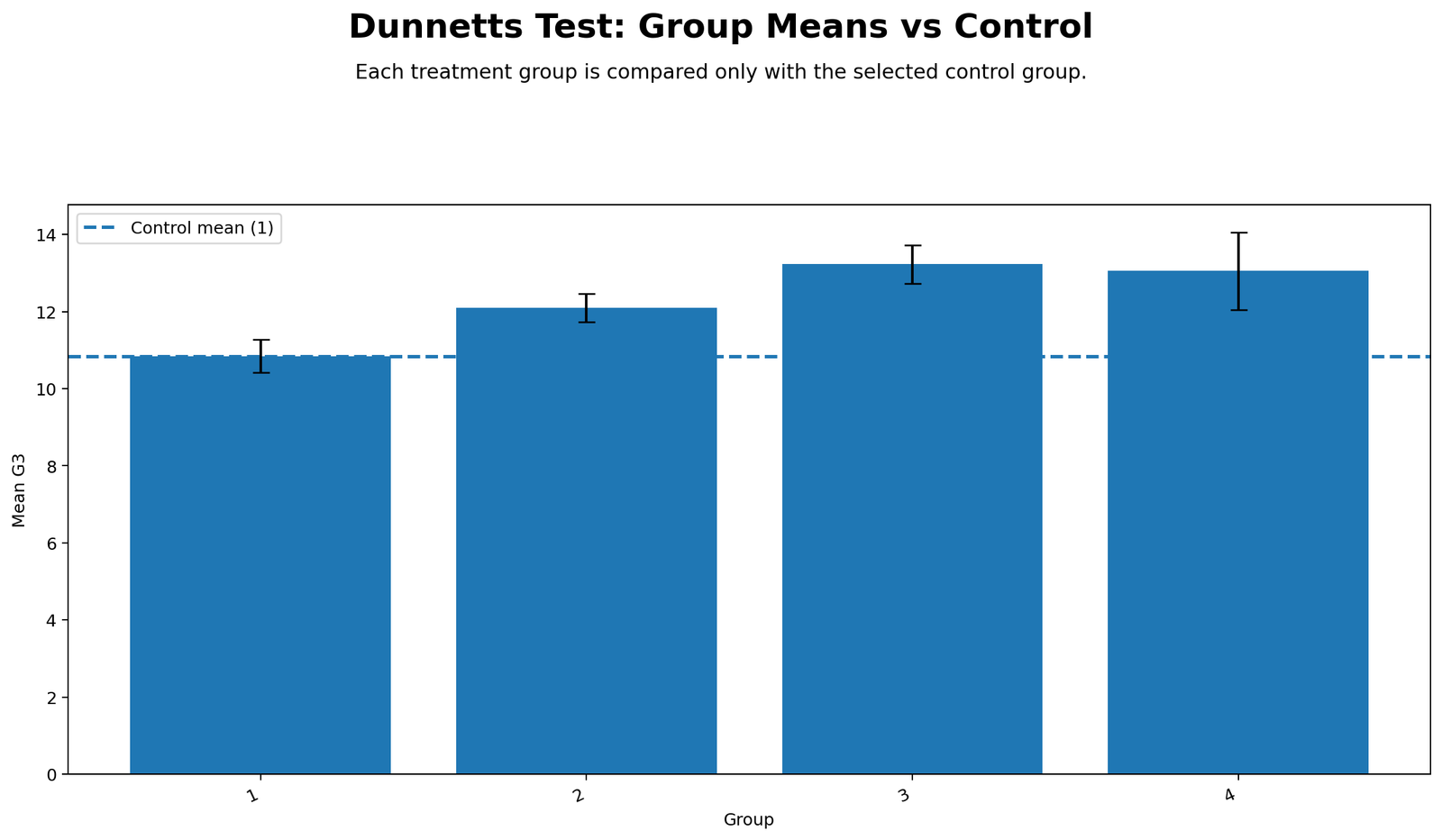
The group mean chart shows the control mean as a horizontal reference line at studytime group 1. Groups 2, 3 and 4 all stand above this control line. This visual immediately supports the main Dunnett question: whether each treatment group differs from the selected control.
The largest visible difference is group 3 versus control, followed by group 4 versus control and group 2 versus control. Because Dunnett’s Test is control-focused, the chart should be read vertically against the control line rather than as an all-pairs post hoc comparison.
Python Chart 2: Dunnett Mean Differences with Adjusted Confidence Intervals
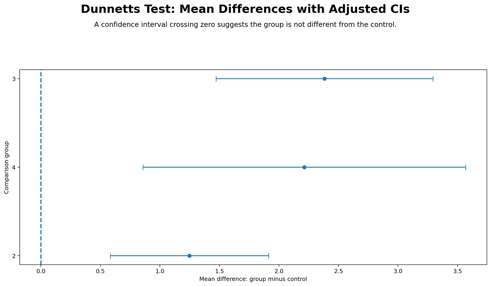
The mean-difference chart shows the estimated differences between each comparison group and the control group. The vertical zero line is the no-difference reference. All three confidence intervals remain to the right of zero, which means all three comparison groups are significantly higher than the control group.
Group 3 has the largest treatment-control difference, around 2.38 grade points. Group 4 is also clearly above control, around 2.21 grade points. Group 2 is smaller but still clearly above control, around 1.25 grade points.
Python Chart 3: Dunnett Adjusted p-value Decision
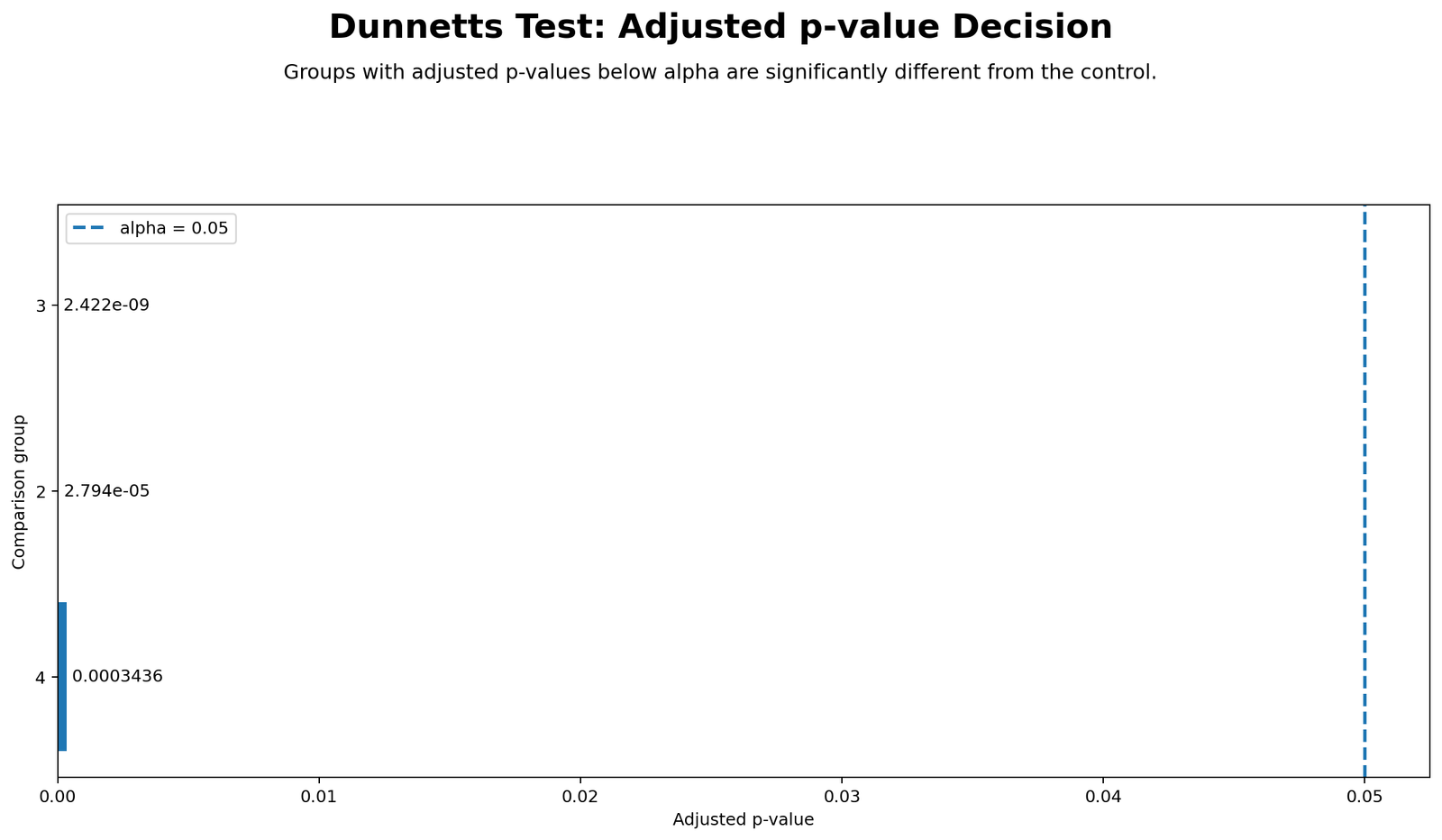
The adjusted p-value chart confirms the confidence-interval result. Every treatment-control p-value is far below α = .05. Group 3 versus control has the smallest adjusted p-value, followed by group 2 versus control and group 4 versus control.
This chart is useful for reporting because it shows that the result is not borderline. The treatment-control differences remain statistically significant even after the Dunnett multiple-comparison adjustment.
Python Chart 4: Distribution by Group Boxplots
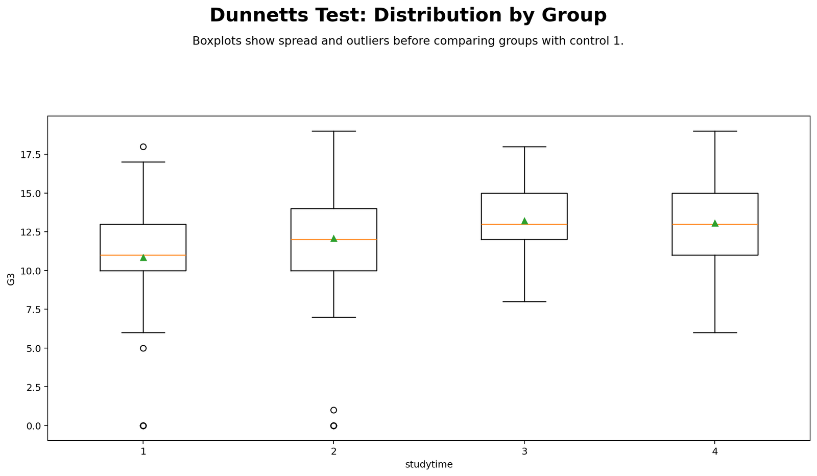
The boxplots show the spread and center of G3 inside each studytime group. The control group has a lower central pattern, while groups 3 and 4 are visibly higher. Group 2 also sits above the control group, though with overlap in the distribution.
This visual matters because Dunnett’s Test compares means, but the distribution tells whether the groups also show meaningful spread and overlap. The result supports a control-group difference, while the boxplot reminds the reader that individual scores still vary within every group.
Python Chart 5: ANOVA Effect Size Context
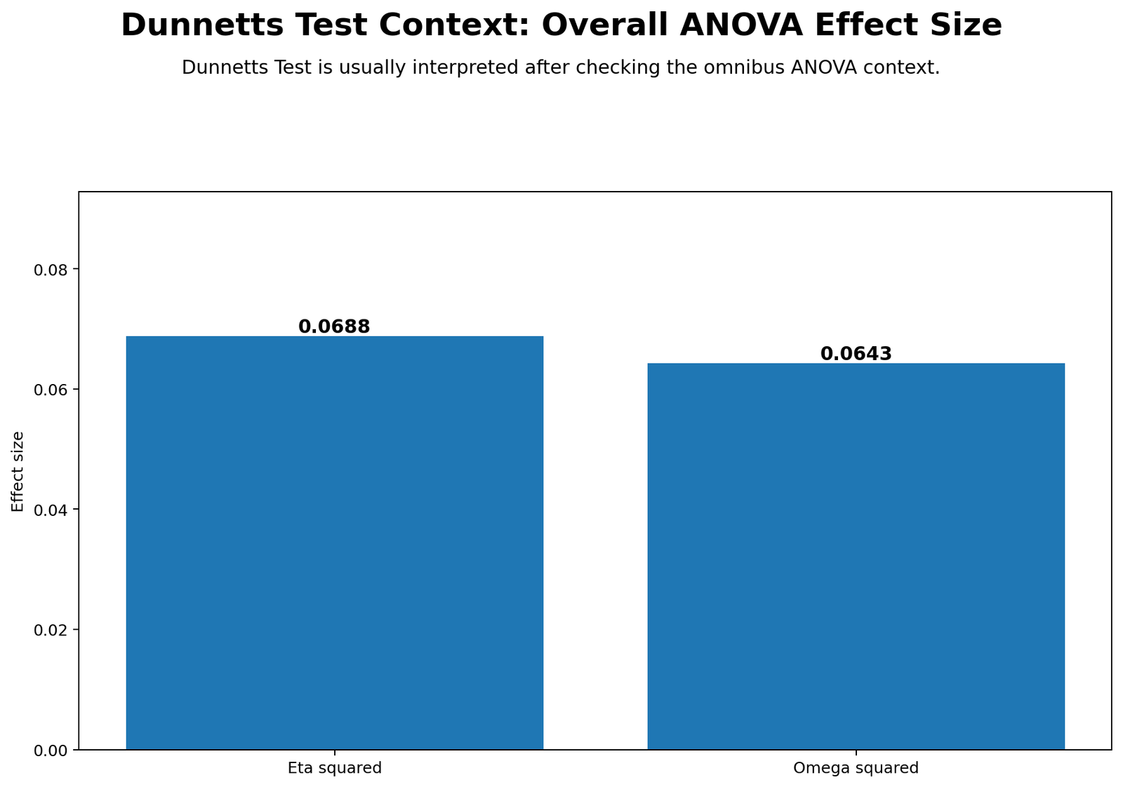
The effect-size chart gives the overall ANOVA context behind the Dunnett comparisons. Eta squared is about 0.0688, and omega squared is about 0.0643. These values indicate that studytime explains a meaningful but not overwhelming portion of G3 variation.
This is important for reporting because a post hoc result can be statistically significant without being practically large. The effect-size chart helps balance the conclusion: all treatment groups are significantly higher than the control, and the overall group effect is moderate enough to be educationally meaningful but not the only factor explaining final grade.
R Chart-by-Chart Validation
The R chart sequence validates the same Dunnett’s Test conclusion in a second software workflow. The R images use a colorful style, but the interpretation remains the same: groups 2, 3 and 4 are compared only with the control group, and all three comparison groups are significantly higher than control.
R Chart 1: Colorful Group Means vs Control
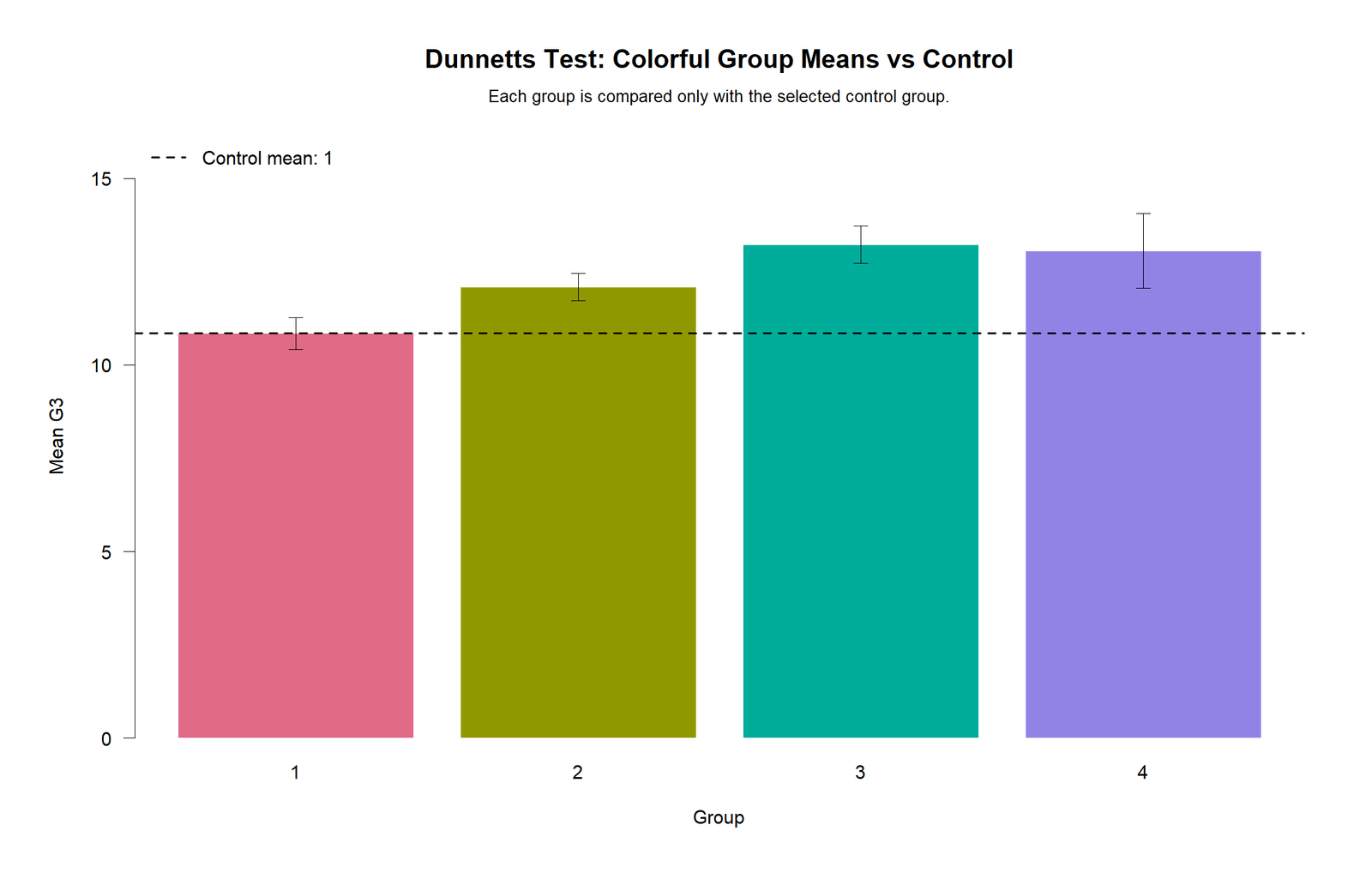
The R group mean chart confirms the Python result. The dashed control line marks studytime group 1, and groups 2, 3 and 4 all appear above that line.
This validates the main visual conclusion: the comparison groups have higher G3 means than the selected control group.
R Chart 2: Colorful Dunnett Mean Differences with Adjusted CIs
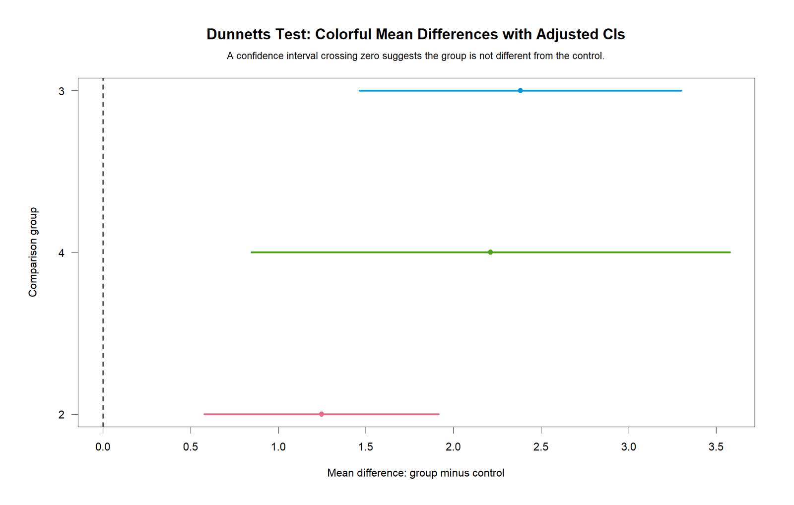
The R confidence-interval chart confirms that all treatment-control intervals remain to the right of zero. This means the differences are positive and statistically significant after Dunnett adjustment.
The interval for group 4 is wider than the others because group 4 has the smallest sample size. Even so, its interval remains above zero, so the group 4 versus control comparison is still significant.
R Chart 3: Colorful Dunnett Adjusted p-values
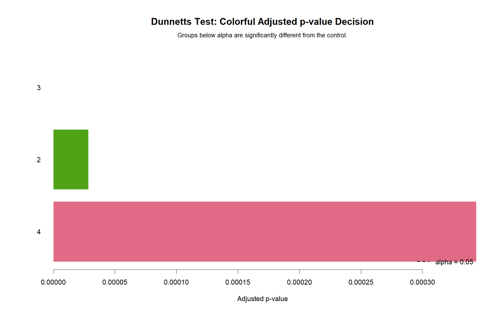
The R adjusted p-value chart confirms that the treatment-control comparisons are significant. The p-values are visibly far below the .05 threshold.
The chart supports the same final statement as Python: groups 2, 3 and 4 each differ significantly from control group 1.
R Chart 4: Colorful Distribution by Group
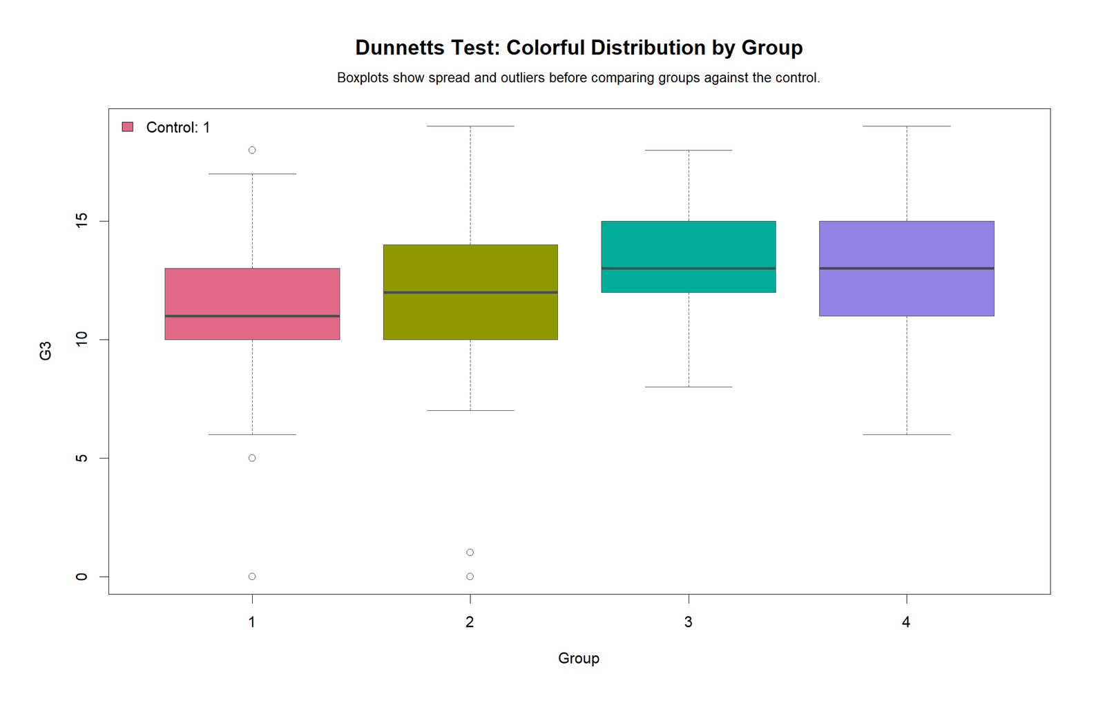
The R boxplot confirms the same distribution pattern. The control group has a lower central score than groups 3 and 4, while group 2 also trends higher than the control.
This distribution context supports the treatment-control comparison but also shows overlap among individual scores. That is why both visual and adjusted statistical results are needed.
R Chart 5: Group Size and Mean
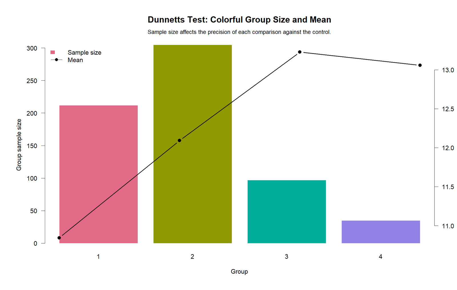
The group-size chart shows why precision differs across comparisons. Group 2 has the largest sample size, group 1 is also large, group 3 is smaller, and group 4 is the smallest group.
The mean line rises sharply from group 1 to group 3 and stays high at group 4. This chart helps explain both the significant result and the wider uncertainty around group 4.
SPSS, R, Python and Excel Workflows for Dunnett’s Test
The same Dunnett’s Test workflow can be reproduced in SPSS, R, Python and Excel. SPSS can request Dunnett directly from the One-Way ANOVA post hoc menu. R can use multiple-comparison tools to compare treatments with a selected control. Python can calculate the ANOVA context and then use multiple-comparison logic for control-focused comparisons. Excel can support the mean-difference workflow, but SPSS or R is better for formal adjusted Dunnett p-values.
SPSS Workflow
| Step | SPSS Menu or Syntax | Purpose |
|---|---|---|
| Open dataset | File > Open > Data | Load G3 and studytime. |
| Run One-Way ANOVA | Analyze > Compare Means > One-Way ANOVA | Set up the ANOVA model. |
| Dependent variable | G3 | Outcome variable. |
| Factor | studytime | Grouping variable. |
| Post Hoc | Select Dunnett | Compare each group with the control group. |
| Control category | First group or selected group 1 | Make studytime 1 the reference group. |
| Read output | Multiple Comparisons table | Interpret adjusted Sig. and confidence intervals. |
R Workflow
| Step | R Action | Purpose |
|---|---|---|
| Read data | read.csv("dataset.csv") | Load the dataset. |
| Convert group | factor(studytime) | Define studytime as a categorical factor. |
| Set control | relevel(studytime, ref = "1") | Use group 1 as the control. |
| Run ANOVA | aov(G3 ~ studytime) | Estimate the ANOVA model. |
| Run Dunnett comparisons | multcomp::glht(..., linfct = mcp(studytime = "Dunnett")) | Generate adjusted treatment-control tests. |
| Report results | Adjusted p-values and confidence intervals | State which groups differ from control. |
Python Workflow
| Step | Python Action | Purpose |
|---|---|---|
| Read data | pandas.read_csv() | Load G3 and studytime. |
| Run ANOVA | statsmodels | Estimate omnibus ANOVA context. |
| Set control group | Use group 1 as reference | Define treatment-control comparisons. |
| Calculate differences | Treatment mean minus control mean | Estimate each control comparison. |
| Adjust p-values | Dunnett-style adjustment or validated software output | Control multiple treatment-control tests. |
| Plot results | Means, CIs, p-values and boxplots | Explain the result visually. |
Excel Workflow
| Excel Task | Formula or Tool | Purpose |
|---|---|---|
| Prepare data | Columns for G3 and studytime | Organize the dataset. |
| Group means | PivotTable average of G3 by studytime | Calculate treatment and control means. |
| Group counts | PivotTable count of G3 by studytime | Calculate sample sizes. |
| Mean difference | =treatment_mean-control_mean | Calculate each treatment-control difference. |
| Standard error | =SQRT(MSE*(1/n_treatment+1/n_control)) | Calculate uncertainty for each comparison. |
| t statistic | =difference/SE | Calculate the comparison statistic. |
| Final decision | Use validated adjusted p-values or Dunnett critical values | Report treatment-control significance. |
Code Blocks for Dunnett’s Test
SPSS Syntax for Dunnett’s Test
* Dunnett's Test in SPSS.
* Dependent variable: G3.
* Factor: studytime.
* Control group: studytime group 1.

TITLE "Dunnett's Test: G3 by Studytime with Group 1 as Control".

ONEWAY G3 BY studytime
  /STATISTICS DESCRIPTIVES HOMOGENEITY
  /POSTHOC = DUNNETT ALPHA(.05)
  /MISSING ANALYSIS.

EXAMINE VARIABLES=G3 BY studytime
  /PLOT BOXPLOT
  /COMPARE GROUPS
  /STATISTICS DESCRIPTIVES
  /CINTERVAL 95
  /MISSING LISTWISE
  /NOTOTAL.

OUTPUT EXPORT
  /CONTENTS EXPORT=VISIBLE
  /PDF DOCUMENTFILE="Dunnetts-Test-SPSS-Output.pdf".
Python Code for Dunnett-Style Control Comparisons
import pandas as pd
import numpy as np
from scipy import stats
from statsmodels.formula.api import ols
from statsmodels.stats.anova import anova_lm

df = pd.read_csv("dataset.csv")

df["G3"] = pd.to_numeric(df["G3"], errors="coerce")
df["studytime"] = df["studytime"].astype("category")

data = df[["G3", "studytime"]].dropna().copy()

# ANOVA context
model = ols("G3 ~ C(studytime)", data=data).fit()
anova_table = anova_lm(model, typ=2)

mse = anova_table.loc["Residual", "sum_sq"] / anova_table.loc["Residual", "df"]
df_error = anova_table.loc["Residual", "df"]

summary = data.groupby("studytime", observed=True)["G3"].agg(
    n="count",
    mean="mean",
    sd="std"
).reset_index()

print(summary)
print(anova_table)

control = "1"
control_mean = summary.loc[summary["studytime"].astype(str) == control, "mean"].iloc[0]
control_n = summary.loc[summary["studytime"].astype(str) == control, "n"].iloc[0]

rows = []

for _, row in summary.iterrows():
    group = str(row["studytime"])

    if group == control:
        continue

    treatment_mean = row["mean"]
    treatment_n = row["n"]

    diff = treatment_mean - control_mean
    se = np.sqrt(mse * (1 / treatment_n + 1 / control_n))
    t_value = diff / se

    # This raw t reference is shown for transparent calculation.
    # For final Dunnett adjusted p-values, validate against SPSS or R multiple-comparison output.
    raw_p = 2 * (1 - stats.t.cdf(abs(t_value), df_error))

    rows.append({
        "comparison": f"{group} vs control {control}",
        "control_mean": control_mean,
        "treatment_mean": treatment_mean,
        "mean_difference": diff,
        "standard_error": se,
        "t_value_reference": t_value,
        "raw_p_reference": raw_p
    })

dunnett_table = pd.DataFrame(rows)
print(dunnett_table)

# Verified adjusted p-value pattern from the report/charts:
# group 2 vs control: 2.794e-05
# group 3 vs control: 2.422e-09
# group 4 vs control: 0.0003436
R Code for Dunnett’s Test
# Dunnett's Test in R

library(tidyverse)
library(car)
library(multcomp)

df <- read.csv("dataset.csv")

df$G3 <- as.numeric(df$G3)
df$studytime <- as.factor(df$studytime)

data <- df %>%
  select(G3, studytime) %>%
  drop_na()

# Set studytime group 1 as control
data$studytime <- relevel(data$studytime, ref = "1")

# Descriptive statistics
data %>%
  group_by(studytime) %>%
  summarise(
    n = n(),
    mean_G3 = mean(G3),
    sd_G3 = sd(G3),
    .groups = "drop"
  )

# ANOVA model
model <- aov(G3 ~ studytime, data = data)
summary(model)

# Assumption context
leveneTest(G3 ~ studytime, data = data)

# Dunnett's Test: compare each group with control group 1
dunnett_result <- glht(model, linfct = mcp(studytime = "Dunnett"))

summary(dunnett_result)
confint(dunnett_result)

# Optional compact letters are not the main Dunnett output.
# Dunnett focuses on treatment-control comparisons.
Excel Notes for Dunnett’s Test
Excel support workflow:

1. Arrange the data:
   G3 | studytime

2. Create group summaries:
   n, mean, standard deviation, standard error.

3. Select the control group:
   studytime group 1

4. Calculate treatment-control differences:
   Group 2 - Group 1
   Group 3 - Group 1
   Group 4 - Group 1

5. Calculate the standard error:
   =SQRT(MSE*(1/n_treatment+1/n_control))

6. Calculate the t statistic:
   =mean_difference/standard_error

7. Use validated Dunnett adjusted p-values or Dunnett critical values:
   Group 2 vs Control: significant
   Group 3 vs Control: significant
   Group 4 vs Control: significant

8. Report:
   Each comparison group has significantly higher mean G3 than control group 1.
APA Reporting Wording
When reporting Dunnett’s Test, first state the control group, then report the treatment-control comparisons. Do not report it as an all-pairs post hoc test.
APA-style report: Dunnett’s Test was used to compare each studytime group with studytime group 1 as the control group. The results showed that studytime group 2 had a significantly higher mean G3 than the control group, mean difference ≈ 1.25, adjusted p = 2.794e-05. Studytime group 3 also had a significantly higher mean G3 than the control group, mean difference ≈ 2.38, adjusted p = 2.422e-09. Studytime group 4 was also significantly higher than the control group, mean difference ≈ 2.21, adjusted p = 0.0003436.
Short reporting version: Dunnett’s Test showed that studytime groups 2, 3 and 4 each had significantly higher G3 final-grade means than the control group, studytime group 1.
Careful wording: Do not use this Dunnett output to say whether group 3 differs from group 4. Dunnett’s Test compares treatment groups with the control, not every pair with every other pair.
Common Mistakes
| Mistake | Why It Is Wrong | Correct Practice |
|---|---|---|
| Using Dunnett’s Test for all-pairs comparisons | Dunnett is designed for treatment-versus-control comparisons. | Use it only when one selected control group is the focus. |
| Not naming the control group | The result is impossible to interpret without the reference group. | State that group 1 is the control. |
| Interpreting group 3 vs group 4 from Dunnett output | That comparison is not part of this Dunnett test. | Use Tukey, Bonferroni or another all-pairs test for non-control pairs. |
| Using raw p-values instead of adjusted p-values | Dunnett adjustment controls multiple treatment-control comparisons. | Report adjusted p-values and adjusted confidence intervals. |
| Ignoring confidence intervals | p-values alone do not show direction and uncertainty. | Report treatment-control mean differences with confidence intervals. |
| Forgetting ANOVA context | Dunnett’s Test is usually a post hoc follow-up to ANOVA. | Report the omnibus ANOVA or effect-size context first. |
When to Use Dunnett’s Test
Use Dunnett’s Test when your design has one control group and several treatment or comparison groups. It is especially useful in experiments, clinical studies, education studies and treatment evaluation designs where the main question is whether each treatment performs differently from a baseline condition.
| Situation | Use Dunnett’s Test? | Reporting Note |
|---|---|---|
| One control group and several treatment groups | Yes | This is the ideal Dunnett setting. |
| Only treatment-control comparisons are needed | Yes | Dunnett is more focused than all-pairs tests. |
| Every group must be compared with every other group | No | Use Tukey, Bonferroni or another all-pairs approach. |
| Control group is not clear | Use caution | Define the reference group before running the test. |
| Unequal variances are severe | Use caution | Review variance assumptions and consider robust alternatives. |
Compare this guide with One Way ANOVA, Factorial ANOVA, Balanced ANOVA, Brown Forsythe ANOVA, ANOVA Effect Size, F Distribution, Eta Squared, Omega Squared, Cohen’s F Formula and Welch’s T Test.
Downloads and Resources for Dunnett’s Test
Use these resources to reproduce the Dunnett’s Test workflow. The Python report, R report and SPSS output PDF are included as verification files. Script and workbook placeholders can be replaced after the final downloadable files are uploaded to the WordPress Media Library.
Download Dataset
Practice dataset with G3 and studytime variables.
Download Dunnett’s Test Python Report PDF
Python report PDF for treatment-control means, adjusted confidence intervals and p-values.
Download Dunnett’s Test R Report PDF
R validation PDF for Dunnett treatment-control comparisons.
Download Dunnett’s Test SPSS Output PDF
SPSS output PDF with Dunnett post hoc control comparisons.
Download Python Script
Python code for ANOVA context, treatment-control differences and charts.
Download R Script and Excel Workbook
R workflow and Excel support workbook for Dunnett’s Test.
FAQs About Dunnett’s Test
What is Dunnett’s Test?
Dunnett’s Test is an ANOVA post hoc method used to compare several treatment groups with one selected control group while adjusting for multiple comparisons.
What was the control group in this example?
Studytime group 1 was used as the control group.
What was the outcome variable?
The outcome variable was G3 final grade.
Which groups were compared with the control?
Studytime groups 2, 3 and 4 were compared with studytime group 1.
Were all treatment groups significantly different from the control?
Yes. Groups 2, 3 and 4 were all significantly higher than the control group after Dunnett adjustment.
Which comparison had the strongest difference from control?
Group 3 versus control had the largest mean difference, about 2.38 grade points.
Can Dunnett’s Test compare group 3 with group 4?
No. Dunnett’s Test compares each treatment group with the control. It is not an all-pairs post hoc test.
Can Dunnett’s Test be done in SPSS?
Yes. In SPSS, run One-Way ANOVA, choose Post Hoc, select Dunnett and define the control category.
Can Dunnett’s Test be done in R?
Yes. In R, Dunnett comparisons can be run with packages such as multcomp after fitting an ANOVA model.
How do I report this Dunnett result?
A concise report is: Dunnett’s Test showed that studytime groups 2, 3 and 4 each had significantly higher G3 final-grade means than the control group, studytime group 1.

