
ANOVA effect size, formula and worked example
Partial Eta Squared: Formula, Interpretation & Examples
Partial eta squared (ηp²) measures the size of one ANOVA effect relative to that effect plus its error. Use the formula, interpretation thresholds, verified example and SPSS, R, Python and Excel steps below.
Quick Answer: Partial Eta Squared Result
The worked Partial Eta Squared output shows three ANOVA effects. The school effect has the largest partial eta squared, ηp² = 0.06723, with F = 46.2 and p = 2.445e-11. The studytime effect has ηp² = 0.05498, with F = 12.43 and p = 6.557e-08. The studytime × school interaction has ηp² = 0.001699, with F = 0.3636 and p = 0.7793.
The result means that school and studytime both contribute meaningful explainable variation in G3, while the interaction contributes almost no practical effect in this model. School is labelled medium in the summary table, studytime is labelled small, and the interaction is labelled very small.
Final interpretation: Partial eta squared shows that school has the strongest effect on G3 in this model, studytime also contributes meaningfully, and the studytime × school interaction is negligible. The practical conclusion is that school differences and studytime differences matter separately, but the studytime pattern does not change strongly by school.
Important reporting point: Partial eta squared is effect-specific. It should not be read exactly like total variance explained in a simple one-way ANOVA. Each value describes the effect relative to that effect plus its error term.
Table of Contents
- What Is Partial Eta Squared?
- Partial Eta Squared Formula
- ANOVA Hypotheses Behind Partial Eta Squared
- Dataset and ANOVA Variables Used
- SPSS Output Interpretation for Partial Eta Squared
- Python Chart-by-Chart Interpretation
- R Chart-by-Chart Validation
- SPSS, R, Python and Excel Workflows
- Code Blocks for Partial Eta Squared
- APA Reporting Wording
- Common Mistakes
- When to Use Partial Eta Squared
- Downloads and Resources
- Related Guides
- FAQs
What Is Partial Eta Squared?
Partial Eta Squared is an effect-size measure commonly reported in ANOVA, ANCOVA, MANOVA follow-up tests, mixed ANOVA and factorial ANOVA. It estimates the proportion of effect-plus-error variation associated with a specific effect. In simple terms, it answers: how large is this ANOVA effect after comparing its sum of squares with the error left for that effect?
In this example, the model tests studytime, school, and studytime × school for the outcome G3. Partial eta squared is calculated separately for each effect. The school value is largest, the studytime value is slightly smaller, and the interaction value is nearly zero.
Partial eta squared is especially useful when a model has more than one effect. A normal one-way ANOVA can use eta squared or omega squared, but factorial models, ANCOVA models and repeated-measures designs often report partial eta squared because each effect has its own comparison with error.
Simple definition: Partial eta squared is an ANOVA effect size for one effect at a time. In this example, school has partial η² = 0.06723, studytime has partial η² = 0.05498, and the studytime × school interaction has partial η² = 0.001699.
Partial Eta Squared connects directly with One Way ANOVA, One Way ANCOVA, Factorial ANOVA, Mixed ANOVA, Mixed MANOVA, Nested ANOVA, ANOVA Effect Size, Eta Squared, and Omega Squared.
Partial Eta Squared Formula
The common formula for partial eta squared divides the sum of squares for one effect by the sum of squares for that effect plus the error sum of squares.
The formula is effect-specific. That means the value for school, the value for studytime and the value for the interaction are calculated separately. Each value describes how large that particular effect is in relation to the unexplained error used for that effect.
Eta Squared vs Partial Eta Squared
Eta squared compares an effect with total variation. Partial eta squared compares an effect with effect-plus-error variation. Because of this difference, partial eta squared is often larger than eta squared in multi-effect designs and should not be interpreted as the same measure.
Interpretation Bands
The interpretation chart uses the common rule-of-thumb bands. School, at 0.06723, sits slightly above the medium threshold. Studytime, at 0.05498, is close to the medium threshold but labelled small in the table. The interaction, at 0.001699, is very small.
| Effect | df | SS | F | p | Partial η² | Label |
|---|---|---|---|---|---|---|
| studytime | 3 | 341.2 | 12.43 | 6.557e-08 | 0.05498 | Small |
| school | 1 | 422.8 | 46.2 | 2.445e-11 | 0.06723 | Medium |
| studytime × school | 3 | 9.982 | 0.3636 | 0.7793 | 0.001699 | Very small |
ANOVA Hypotheses Behind Partial Eta Squared
Partial eta squared itself is an effect size, not a p-value test. The p-value tests whether the effect is statistically significant. Partial eta squared then describes how large that effect is.
| Effect | Null Hypothesis | Alternative Hypothesis | Decision in This Output |
|---|---|---|---|
| studytime | Mean G3 is equal across studytime groups after model adjustment. | At least one studytime group differs. | Significant, p = 6.557e-08. |
| school | Mean G3 is equal across schools after model adjustment. | School groups differ in mean G3. | Significant, p = 2.445e-11. |
| studytime × school | The studytime effect is the same across schools. | The studytime effect changes by school. | Not significant, p = 0.7793. |
Decision for this example: The main effects of school and studytime are statistically significant. The interaction is not statistically significant and has a very small partial eta squared. The model supports separate school and studytime effects, not a strong interaction pattern.
Dataset and ANOVA Variables Used
The worked example uses student performance data. The dependent variable is G3 final grade. The effects are studytime, school and studytime × school. This makes it a factorial ANOVA-style effect-size example where partial eta squared is more appropriate than a single overall eta squared.
| Variable | Role | What It Represents | Why It Matters |
|---|---|---|---|
| G3 | Dependent variable | Final grade outcome. | The outcome whose variation is explained by ANOVA effects. |
| studytime | Main effect | Four studytime groups. | Shows whether grade means differ by studytime. |
| school | Main effect | School grouping variable. | Shows whether grade means differ by school. |
| studytime × school | Interaction effect | Combined studytime and school pattern. | Shows whether the studytime effect changes across schools. |
The studytime mean chart shows that mean G3 increases from studytime group 1 to group 3, with group 4 remaining high. The cell mean pattern shows GP school above MS school across the studytime groups. These visuals explain why school and studytime have meaningful main effects, while the interaction remains very small.
For supporting concepts, review Descriptive Statistics, Mean Median and Mode, Standard Deviation, Variance, Confidence Interval, P Value, and Null and Alternative Hypothesis.
SPSS Output Interpretation for Partial Eta Squared
The SPSS output should be read from the Tests of Between-Subjects Effects table. In SPSS GLM output, partial eta squared is usually displayed in a column labelled Partial Eta Squared when effect sizes are requested.
SPSS Reading Order
| SPSS Output Area | What to Read | Why It Matters |
|---|---|---|
| Tests of Between-Subjects Effects | Rows for studytime, school and studytime × school. | Shows each model effect separately. |
| F and p columns | F statistic and significance value. | Tests whether each effect is statistically significant. |
| Partial Eta Squared column | Effect-size value for each effect. | Shows practical size of each effect. |
| Estimated means or descriptives | Group means and cell means. | Shows the direction behind each effect. |
| Residual diagnostics | Residual plots and normality checks. | Shows assumption context. |
SPSS Interpretation Summary
| Effect | p-value | Partial Eta Squared | SPSS Interpretation |
|---|---|---|---|
| school | 2.445e-11 | 0.06723 | School has the largest effect and is labelled medium. |
| studytime | 6.557e-08 | 0.05498 | Studytime is significant and close to the medium threshold. |
| studytime × school | 0.7793 | 0.001699 | The interaction is not significant and is practically very small. |
The SPSS result should not be reported as one combined number. The correct report gives each effect separately. School and studytime should be discussed as meaningful main effects. The interaction should be described as negligible and not statistically significant.
SPSS interpretation summary: The partial eta squared output shows that school has the largest effect on G3, studytime also has a meaningful effect, and the interaction is almost zero. The practical result is an additive pattern rather than a strong interaction pattern.
Python Chart-by-Chart Interpretation
The Python chart sequence explains partial eta squared through effect-size bars, studytime means, distributions, school-by-studytime cell means, residual diagnostics, interpretation bands and the ANOVA summary table.
Python Chart 1: Partial Eta Squared by ANOVA Effect
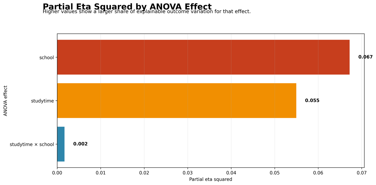
This chart shows that school has the largest partial eta squared value at 0.067. Studytime is second at 0.055, and the interaction is far smaller at about 0.002.
The practical interpretation is direct. School and studytime explain meaningful portions of effect-specific outcome variation, while the interaction does not. The model is mainly explained by separate main effects rather than by a combined studytime-by-school pattern.
Python Chart 2: Mean G3 by Studytime
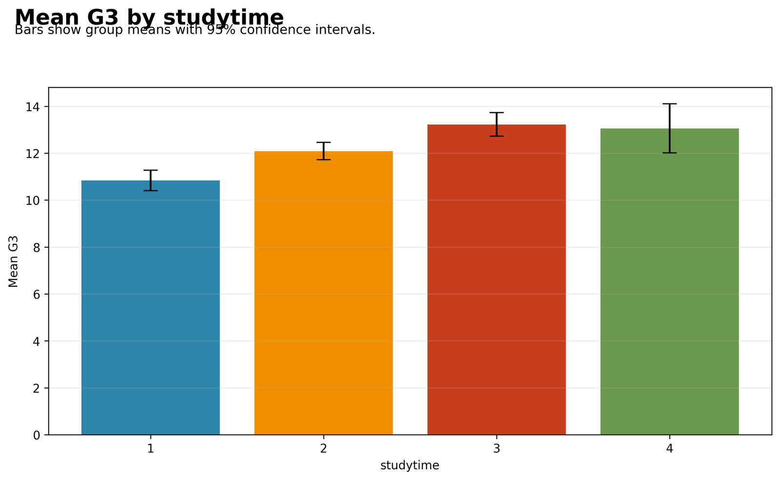
This chart shows the primary studytime pattern. Mean G3 is lowest in studytime group 1, rises in group 2, reaches its highest point in group 3, and remains high in group 4.
The confidence intervals show the uncertainty around each group mean. Group 4 has a visibly wider interval than the other groups, but the mean remains in the high range. This chart explains why studytime has a significant p-value and a partial eta squared near the medium threshold.
Python Chart 3: Distribution of G3 by Studytime
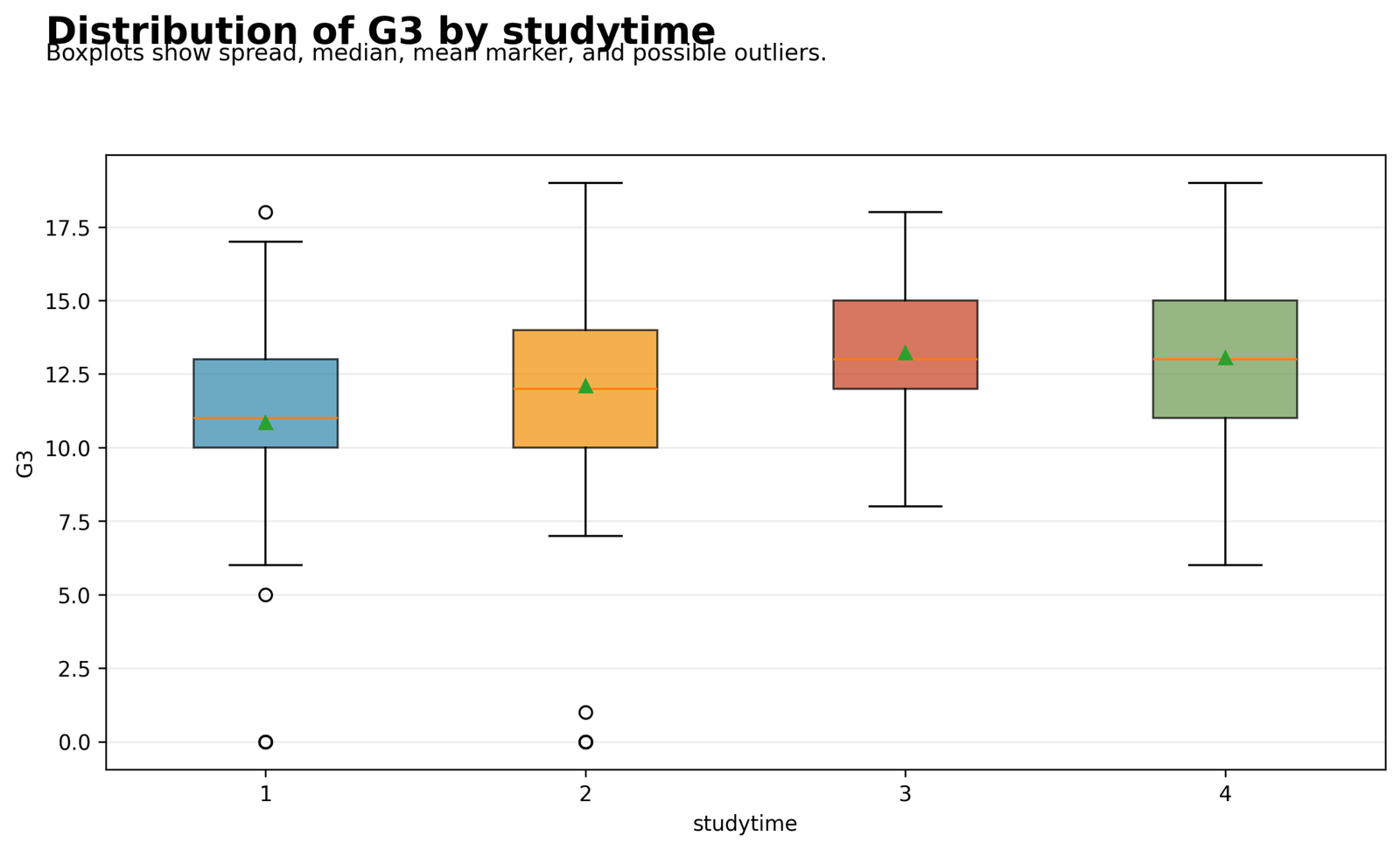
The boxplots show that the center of the G3 distribution shifts upward across higher studytime groups. Groups 3 and 4 are centered higher than groups 1 and 2, while group 1 has the lowest center.
Low outlying values are visible in the lower studytime groups, especially near zero. These low values help explain the residual diagnostic departures seen later. The distributions overlap, so the effect is meaningful but not overwhelmingly large.
Python Chart 4: Cell Mean Pattern for Partial Eta Squared Context
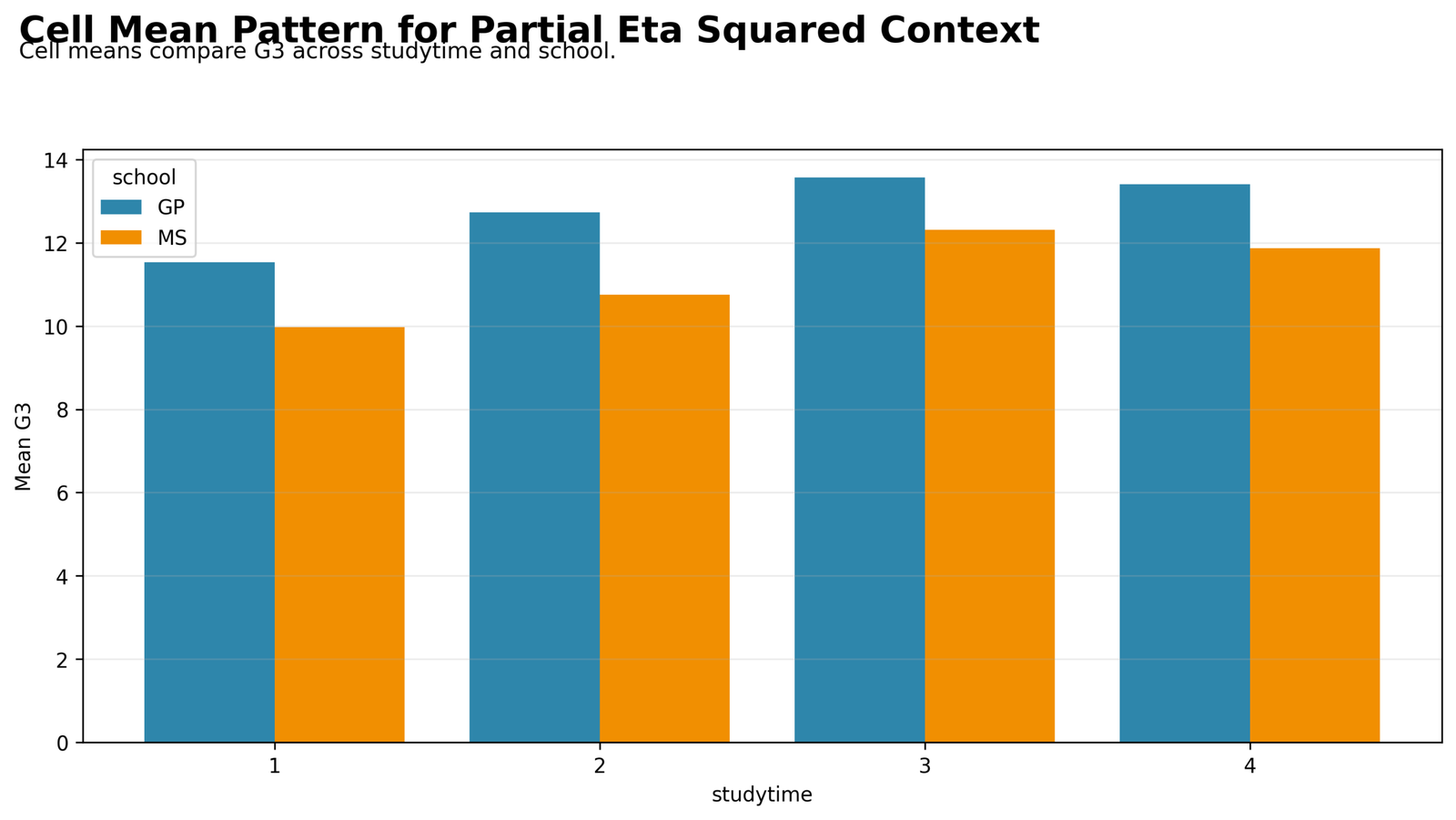
The cell mean chart shows that the GP school bars are higher than the MS school bars across studytime groups. This explains why the school main effect has the largest partial eta squared.
The studytime pattern is also visible within each school. Means generally increase from lower studytime groups to higher studytime groups. However, the gap between school groups does not change dramatically across studytime levels, which supports the very small interaction effect.
Python Chart 5: Residuals vs Fitted Values
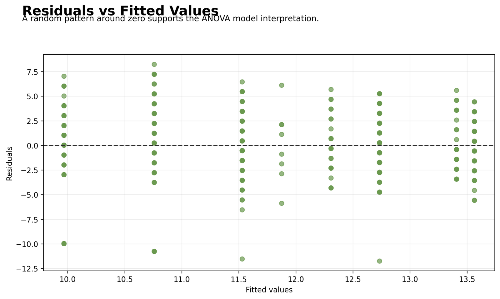
The residuals-versus-fitted chart shows fitted-value bands because the ANOVA model predicts group and cell means. Most residuals are spread around zero, but several negative residuals extend far below the zero line.
The largest negative residuals are close to -12. These cases represent observed G3 scores much lower than the fitted model expected. The chart supports reporting diagnostic caution even though the main effects are significant.
Python Chart 6: Q-Q Plot of ANOVA Residuals
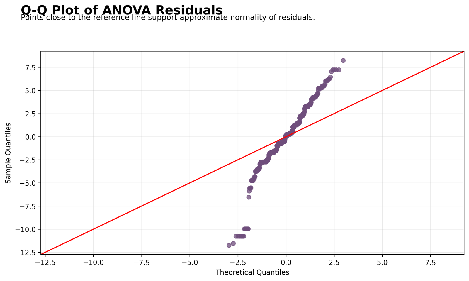
The Q-Q plot shows clear departure from the reference line, especially in the lower tail. The central residuals follow the diagonal pattern more closely than the lowest residuals.
This plot means residual normality is approximate rather than perfect. The model effects can still be reported, but the assumptions section should mention the lower-tail residual departure.
Python Chart 7: Partial Eta Squared Interpretation Bands
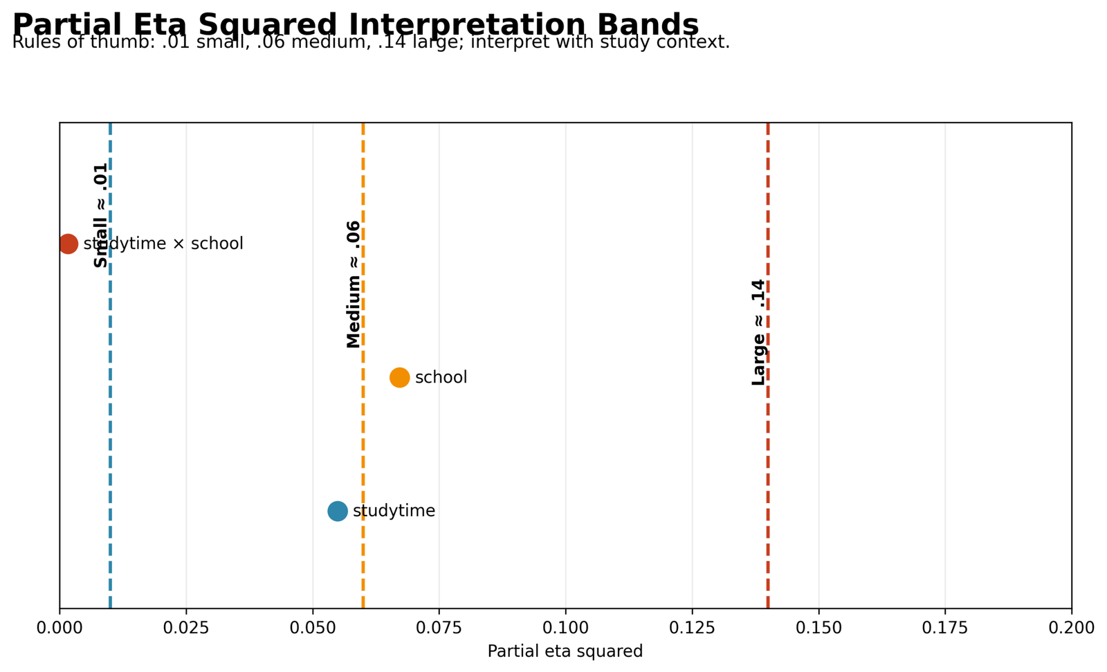
The interpretation band chart places the three effect sizes against the .01, .06 and .14 rule-of-thumb thresholds. School sits just above the medium reference line, studytime is just below the medium reference line, and the interaction is near zero.
This chart is useful because it prevents overstatement. The school and studytime effects are meaningful, but neither approaches the large threshold. The interaction is not practically important in this output.
Python Chart 8: ANOVA Table with Partial Eta Squared
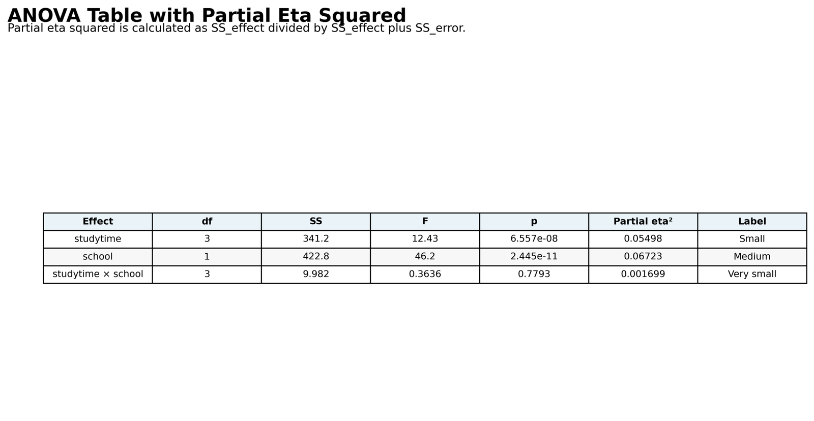
The summary table confirms the formal values. Studytime has df = 3, SS = 341.2, F = 12.43, p = 6.557e-08 and partial η² = 0.05498. School has df = 1, SS = 422.8, F = 46.2, p = 2.445e-11 and partial η² = 0.06723.
The interaction row confirms the weak interaction: df = 3, SS = 9.982, F = 0.3636, p = 0.7793 and partial η² = 0.001699. This table is the best compact source for the final report.
R Chart-by-Chart Validation
The R validation charts repeat the same partial eta squared workflow in a second software environment. They confirm the effect-size ranking, mean pattern, distribution structure, cell mean pattern, diagnostics, interpretation bands and summary table.
R Chart 1: Partial Eta Squared by ANOVA Effect
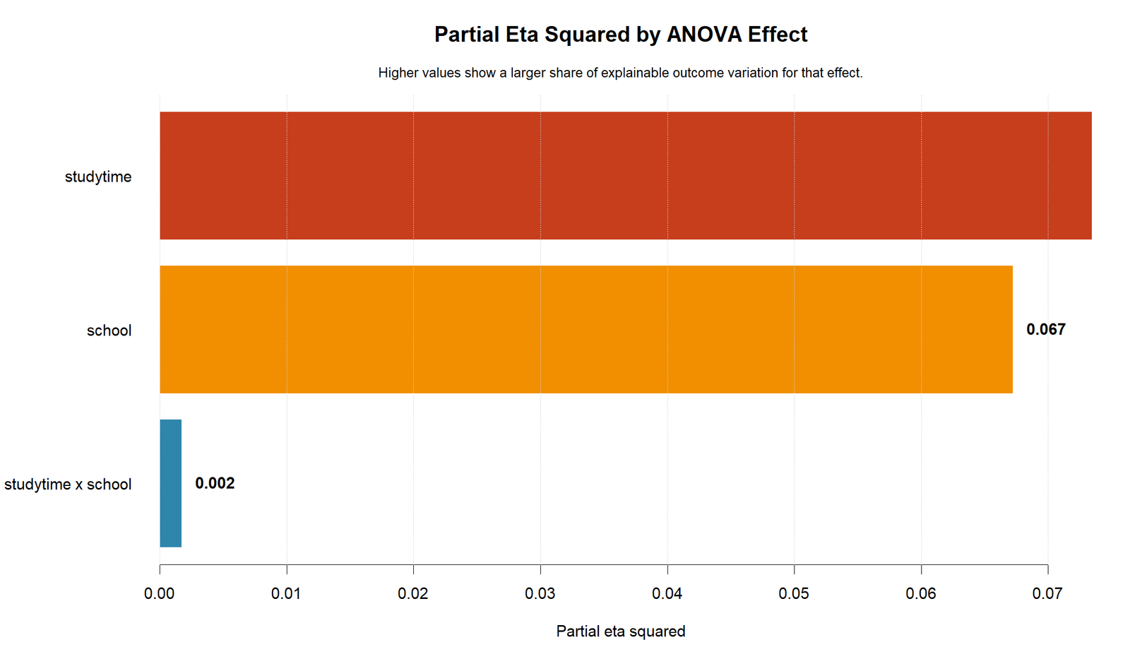
The R chart confirms the same effect-size order. School is largest, studytime is second, and the studytime × school interaction is nearly zero.
This validation supports the main interpretation. The strongest practical effect is the school main effect, followed by studytime, while the interaction does not contribute meaningfully.
R Chart 2: Mean Outcome by Primary Factor
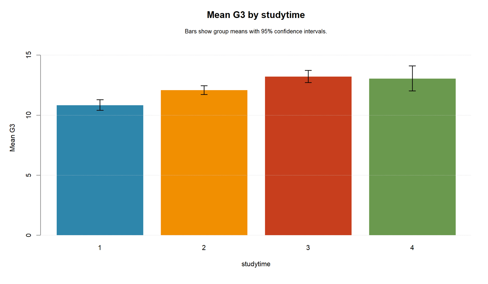
The R mean chart confirms that G3 increases from studytime group 1 toward groups 3 and 4. The mean pattern is the same as the Python output.
This agreement shows that the studytime effect is stable across software workflows. The studytime effect is statistically significant and practically close to the medium threshold.
R Chart 3: Distribution by Primary Factor
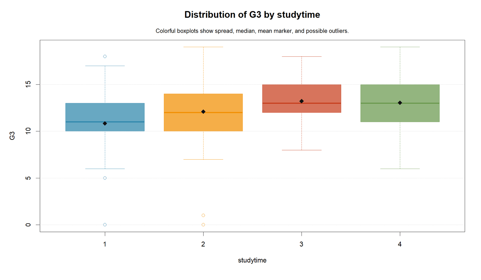
The R boxplots confirm the same distribution pattern. Groups 3 and 4 are centered higher than groups 1 and 2, and low outlying values remain visible in the lower groups.
This validates the visual basis for the studytime effect. The groups differ in center, but the distributions overlap, so the partial eta squared is meaningful rather than large.
R Chart 4: Cell Mean Pattern
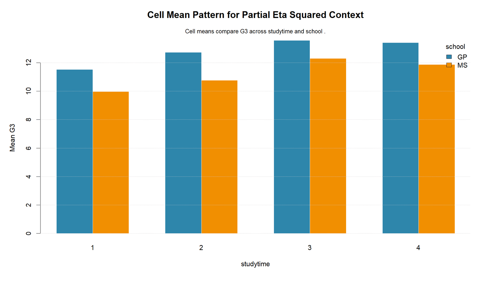
The R cell mean chart confirms that GP school means are generally above MS school means across studytime levels. This supports the significant school main effect.
The interaction remains weak because the school difference does not change enough across studytime groups to create a meaningful studytime × school effect. The chart matches the very small interaction partial eta squared.
R Chart 5: Residuals vs Fitted Values
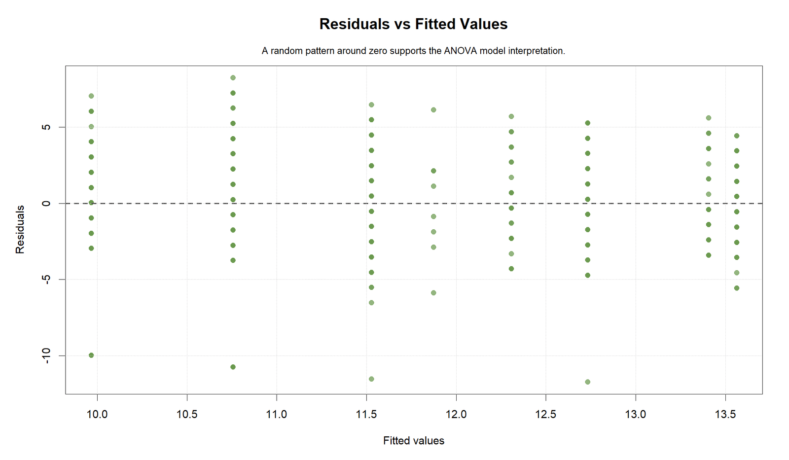
The R residual chart confirms the same fitted-value banding and lower negative residuals. Most residuals are centered around zero, while some observations are much lower than the model expects.
This validation supports the diagnostic conclusion. The model effects are useful, but residual behavior is not perfectly ideal.
R Chart 6: Q-Q Plot of ANOVA Residuals
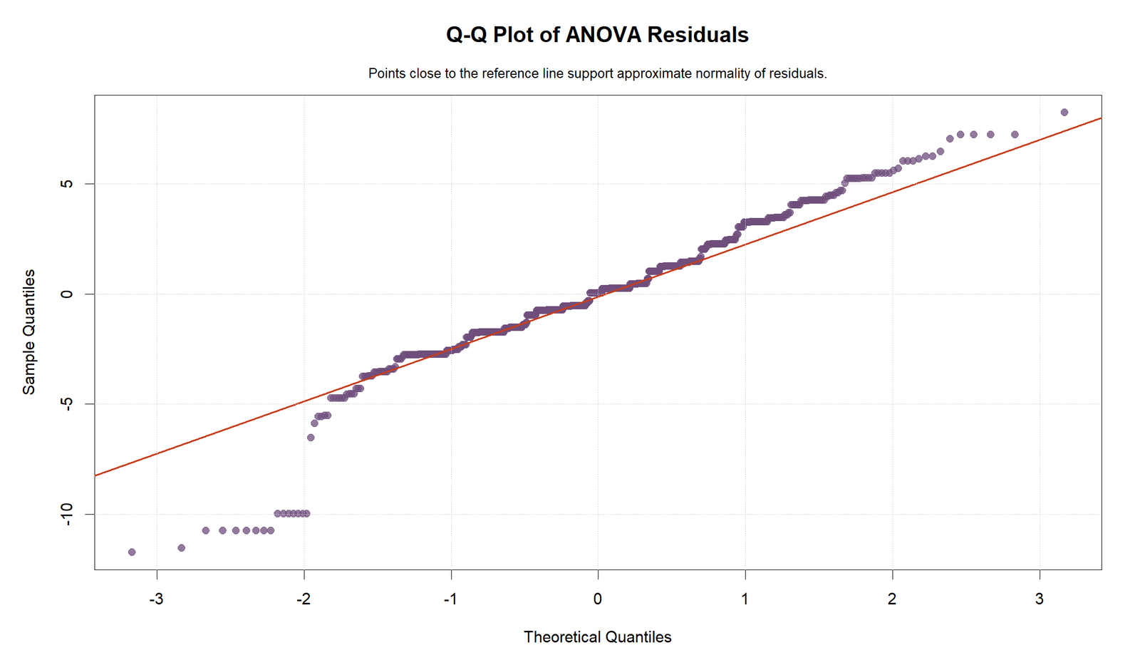
The R Q-Q plot confirms the lower-tail departure visible in the Python chart. The lowest residuals fall away from the reference line more strongly than the central residuals.
The diagnostic message is the same in R and Python. The model can be interpreted, but the assumptions section should mention approximate residual normality rather than perfect normality.
R Chart 7: Partial Eta Squared Interpretation Bands
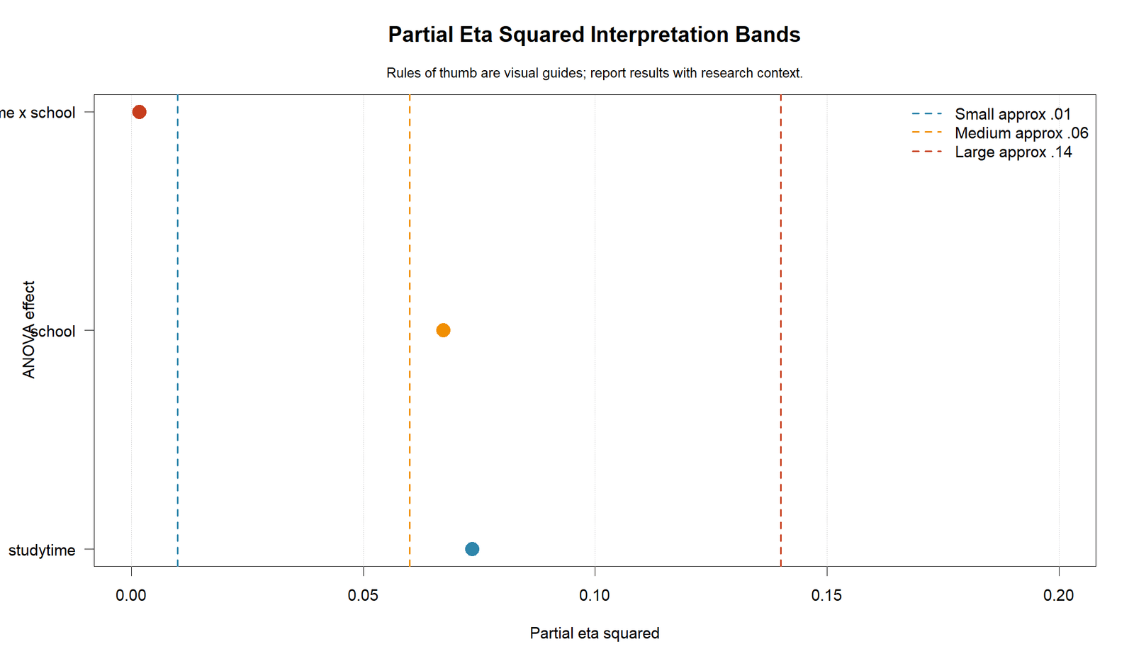
The R interpretation chart confirms that school sits just above the medium threshold, studytime sits just below the medium threshold, and the interaction is almost zero.
This validation supports a careful practical conclusion: school and studytime matter, but the interaction should not be emphasized as meaningful.
R Chart 8: ANOVA Table with Partial Eta Squared
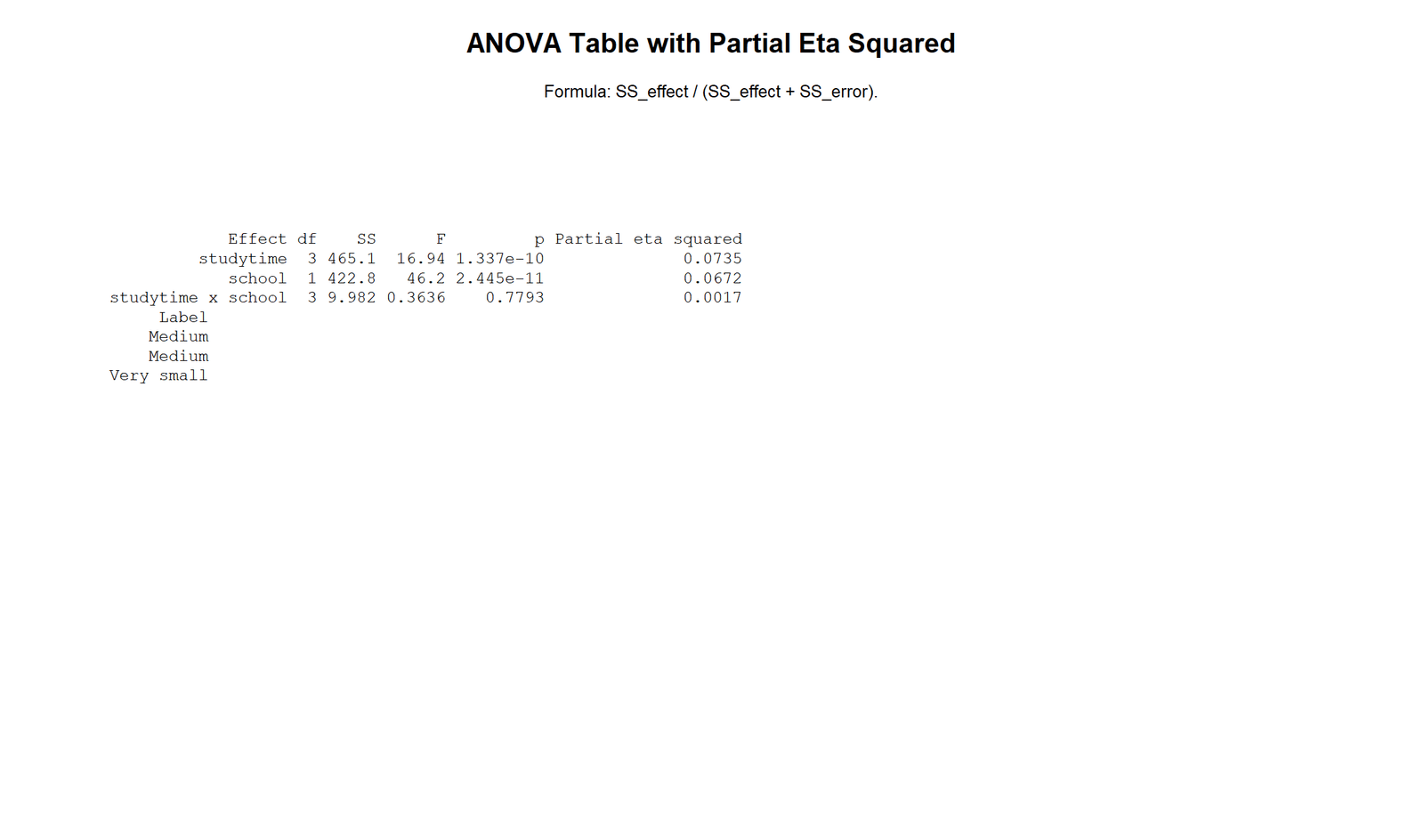
The R summary table confirms the same formal result as the Python table. The main effects of school and studytime are statistically significant, while the interaction is not.
This makes the final report stable across workflows. SPSS, Python and R all support the same interpretation: school has the largest partial eta squared, studytime is meaningful, and the interaction is negligible.
SPSS, R, Python and Excel Workflows for Partial Eta Squared
The same Partial Eta Squared workflow can be reproduced in SPSS, R, Python and Excel. SPSS can display partial eta squared directly. R and Python can calculate it from sums of squares. Excel can calculate it from an ANOVA table when SS effect and SS error are available.
SPSS Workflow
| Step | SPSS Menu or Syntax | Purpose |
|---|---|---|
| Open dataset | File > Open > Data | Load G3, studytime and school. |
| Run GLM Univariate | Analyze > General Linear Model > Univariate | Fit factorial ANOVA model. |
| Set dependent variable | Dependent Variable: G3 | Define outcome. |
| Set fixed factors | Fixed Factors: studytime and school | Define model effects. |
| Request effect size | Options > Estimates of effect size | Display partial eta squared. |
| Read table | Tests of Between-Subjects Effects | Interpret F, p and partial eta squared. |
| Export output | OUTPUT EXPORT | Save SPSS output PDF. |
R Workflow
| Step | R Action | Purpose |
|---|---|---|
| Read data | read.csv("dataset.csv") | Load dataset. |
| Convert factors | as.factor(studytime) and as.factor(school) | Define categorical effects. |
| Fit model | aov(G3 ~ studytime * school) | Fit factorial ANOVA. |
| ANOVA table | summary(model) | Get SS, F and p-values. |
| Effect sizes | effectsize::eta_squared(model, partial = TRUE) | Get partial eta squared. |
| Diagnostics | Residual plots and Q-Q plot | Check assumptions. |
Python Workflow
| Step | Python Action | Purpose |
|---|---|---|
| Read data | pandas.read_csv() | Load G3, studytime and school. |
| Fit model | ols("G3 ~ C(studytime) * C(school)") | Fit factorial ANOVA. |
| ANOVA table | sm.stats.anova_lm(model, typ=2) | Get SS, F and p-values. |
| Partial eta squared | SS_effect / (SS_effect + SS_error) | Calculate effect sizes. |
| Charts | Effect bars, means, cell means and residual plots | Visualize interpretation. |
Excel Workflow
| Excel Task | Formula or Tool | Purpose |
|---|---|---|
| Prepare data | Columns for G3, studytime and school | Create ANOVA input. |
| Create means | PivotTable | Summarize means by factor and cell. |
| Get ANOVA table | Use Excel ToolPak or export from SPSS/R/Python | Obtain SS effect and SS error. |
| Calculate partial eta squared | =SS_effect/(SS_effect+SS_error) | Compute effect size. |
| Create chart | Bar chart of partial eta squared values | Compare effect sizes visually. |
Code Blocks for Partial Eta Squared
SPSS Syntax for Partial Eta Squared
* Partial Eta Squared in SPSS.
* Dependent variable: G3.
* Factors: studytime and school.

TITLE "Partial Eta Squared: G3 by Studytime and School".

UNIANOVA G3 BY studytime school
  /METHOD=SSTYPE(3)
  /INTERCEPT=INCLUDE
  /PRINT=DESCRIPTIVE ETASQ HOMOGENEITY
  /EMMEANS=TABLES(studytime)
  /EMMEANS=TABLES(school)
  /EMMEANS=TABLES(studytime*school)
  /CRITERIA=ALPHA(.05)
  /DESIGN=studytime school studytime*school.

OUTPUT EXPORT
  /CONTENTS EXPORT=VISIBLE
  /PDF DOCUMENTFILE="partial_eta_squared_spss_output.pdf".
Python Code for Partial Eta Squared
import pandas as pd
import statsmodels.api as sm
from statsmodels.formula.api import ols

df = pd.read_csv("dataset.csv")

df["G3"] = pd.to_numeric(df["G3"], errors="coerce")
df["studytime"] = df["studytime"].astype("category")
df["school"] = df["school"].astype("category")

df_model = df.dropna(subset=["G3", "studytime", "school"]).copy()

# Factorial ANOVA model
model = ols("G3 ~ C(studytime) * C(school)", data=df_model).fit()

anova_table = sm.stats.anova_lm(model, typ=2)
print(anova_table)

# Partial eta squared for each effect
ss_error = anova_table.loc["Residual", "sum_sq"]

effects = [row for row in anova_table.index if row != "Residual"]
partial_eta = {}

for effect in effects:
    ss_effect = anova_table.loc[effect, "sum_sq"]
    partial_eta[effect] = ss_effect / (ss_effect + ss_error)

print("Partial eta squared:")
for effect, value in partial_eta.items():
    print(effect, value)

# Fitted values and residuals
df_model["fitted"] = model.fittedvalues
df_model["residual"] = model.resid

print(df_model[["G3", "studytime", "school", "fitted", "residual"]].head())
R Code for Partial Eta Squared
# Partial Eta Squared in R

library(tidyverse)

df <- read.csv("dataset.csv")

df$G3 <- as.numeric(df$G3)
df$studytime <- as.factor(df$studytime)
df$school <- as.factor(df$school)

df_model <- df %>%
  select(G3, studytime, school) %>%
  drop_na()

# Factorial ANOVA
model <- aov(G3 ~ studytime * school, data = df_model)

summary(model)

# Manual partial eta squared from ANOVA table
anova_table <- summary(model)[[1]]
ss_error <- anova_table["Residuals", "Sum Sq"]

partial_eta_studytime <- anova_table["studytime", "Sum Sq"] /
  (anova_table["studytime", "Sum Sq"] + ss_error)

partial_eta_school <- anova_table["school", "Sum Sq"] /
  (anova_table["school", "Sum Sq"] + ss_error)

partial_eta_interaction <- anova_table["studytime:school", "Sum Sq"] /
  (anova_table["studytime:school", "Sum Sq"] + ss_error)

partial_eta_studytime
partial_eta_school
partial_eta_interaction

# Optional package method:
# install.packages("effectsize")
# library(effectsize)
# eta_squared(model, partial = TRUE)

plot(model)
Excel Formulas for Partial Eta Squared
Required values:
SS_effect = sum of squares for the effect
SS_error = residual or error sum of squares

Partial eta squared:
=SS_effect / (SS_effect + SS_error)

Example:
Studytime partial eta squared:
=341.2 / (341.2 + SS_error)

School partial eta squared:
=422.8 / (422.8 + SS_error)

Interaction partial eta squared:
=9.982 / (9.982 + SS_error)

Interpretation bands:
0.01 = small
0.06 = medium
0.14 = large

Report:
Effect name, F statistic, p-value, partial eta squared and practical label.
APA Reporting Wording
When reporting Partial Eta Squared, include the effect name, F statistic, degrees of freedom, p-value, partial eta squared value and a short practical interpretation. For factorial ANOVA, report each effect separately.
APA-style report: A factorial ANOVA was conducted to examine the effects of studytime and school on G3. The school main effect was significant, F(1, error df) = 46.2, p = 2.445e-11, partial η² = 0.06723. The studytime main effect was also significant, F(3, error df) = 12.43, p = 6.557e-08, partial η² = 0.05498. The studytime × school interaction was not significant, F(3, error df) = 0.3636, p = 0.7793, partial η² = 0.001699. Residual diagnostics showed lower-tail departures, so the results were interpreted with diagnostic caution.
Short reporting version: School showed the largest effect on G3, partial η² = 0.06723, followed by studytime, partial η² = 0.05498. The studytime × school interaction was very small, partial η² = 0.001699, and not statistically significant.
Common Mistakes
| Mistake | Why It Is Wrong | Correct Practice |
|---|---|---|
| Reporting only p-values | P-values do not show practical size. | Report F, p and partial eta squared together. |
| Treating partial eta squared as total variance explained | Partial eta squared is effect-specific. | Explain that it uses SS effect divided by SS effect plus SS error. |
| Confusing eta squared and partial eta squared | The denominators are different. | Use Eta Squared for comparison and name the measure clearly. |
| Overstating the interaction | The interaction p = 0.7793 and partial η² = 0.001699. | Describe the interaction as very small and not significant. |
| Ignoring diagnostics | The residual Q-Q plot shows lower-tail departure. | Discuss diagnostics and review Q-Q Plot Normality Check. |
| Using one effect-size rule without context | Thresholds are rough guidelines. | Interpret values with study context, sample size and design. |
When to Use Partial Eta Squared
Use Partial Eta Squared when an ANOVA-style model has multiple effects and each effect needs its own practical-size estimate. It is common in factorial ANOVA, ANCOVA, repeated-measures ANOVA, mixed ANOVA and MANOVA follow-up tests.
| Situation | Use Partial Eta Squared? | Reporting Note |
|---|---|---|
| Factorial ANOVA with main effects and interaction | Yes | Report each effect separately. |
| ANCOVA with covariates | Yes | Report factor and covariate effect sizes. |
| Mixed ANOVA or repeated-measures ANOVA | Yes | Report within, between and interaction effects separately. |
| One-way ANOVA only | Possible, but eta or omega squared may be clearer | Compare with Omega Squared. |
| Need total variance explained | No | Use eta squared or model R² depending on design. |
Partial eta squared should be compared with One Way ANOVA, One Way ANCOVA, Factorial ANOVA, Mixed ANOVA, Nested ANOVA, Fixed Effects ANOVA, ANOVA Effect Size, F Distribution, and Cohen’s F Formula.
Downloads and Resources for Partial Eta Squared
Use these resources to reproduce the Partial Eta Squared workflow. The Python, R and SPSS report PDFs below provide reproducible verification files for the worked example.
Download Partial Eta Squared Python Report PDF
Python report PDF for effect sizes, means, cell patterns and diagnostics.
Download Partial Eta Squared R Report PDF
R validation PDF for partial eta squared interpretation and diagnostics.
Download Partial Eta Squared SPSS Output PDF
SPSS output PDF for ANOVA effect-size reporting.
FAQs About Partial Eta Squared
What is Partial Eta Squared?
Partial Eta Squared is an ANOVA effect-size measure that estimates the size of one effect relative to that effect plus its error variance.
What is the formula for Partial Eta Squared?
The formula is partial η² = SS effect / (SS effect + SS error).
What was the largest partial eta squared in this example?
The largest value was for school, partial η² = 0.06723.
What was the partial eta squared for studytime?
The partial eta squared for studytime was 0.05498.
What was the partial eta squared for the interaction?
The partial eta squared for studytime × school was 0.001699, which is very small.
Was the school effect significant?
Yes. The school effect was significant with p = 2.445e-11.
Was the studytime effect significant?
Yes. The studytime effect was significant with p = 6.557e-08.
Was the interaction significant?
No. The studytime × school interaction had p = 0.7793 and a very small partial eta squared.
Is partial eta squared the same as eta squared?
No. Eta squared uses total variation in the denominator, while partial eta squared uses effect variation plus error variation.
How do I report Partial Eta Squared in APA style?
Report each effect with its F statistic, p-value and partial eta squared, such as: school was significant, F = 46.2, p = 2.445e-11, partial η² = 0.06723.

