
Multiple Linear Regression: Formula, Interpretation, SPSS, Python, R and Excel Guide
Multiple Linear Regression predicts one continuous outcome from several predictors at the same time. This beginner-friendly example predicts final grade G3 for 649 students, explains the regression equation, separates simple and adjusted relationships, interprets eight charts, checks residuals and VIF, and compares the Python core model with the expanded SPSS and Excel specification.
G3 outcome
Core R² = 0.8522
SPSS · Python · R · Excel
Multiple Linear Regression Model Overview
Beginner explanation: simple linear regression predicts an outcome from one predictor. Multiple Linear Regression extends the same idea by including several predictors in one equation. Every coefficient estimates the expected outcome change associated with one predictor while all other predictors are held constant.
In the Python core model, G3 is predicted from G1, G2, studytime, failures, absences, age, school, sex and address. The expanded SPSS and Excel model adds maternal education, paternal education, travel time, health, higher-education intention and internet access.
If you are new to regression, begin with Correlation vs Regression and Pearson Correlation. Correlation measures how two variables move together; Multiple Linear Regression estimates a predictor’s conditional contribution after the other variables are considered.
Quick Answer: Multiple Linear Regression Results
Python core model
- F(9,639) = 409.4514, p < .001
- G2 = 0.8794, p < .001
- G1 = 0.1328, p = .0003
- failures = -0.2266, p = .0170
- sex_M = -0.2037, p = .0493
SPSS and Excel expanded model
- R² = 0.8541; adjusted R² = 0.8507
- F(15,633) = 247.0965, p < .001
- G2 = 0.8757, p < .001
- G1 = 0.1328, p = .0003
- failures = -0.2186, p = .0227
Plain-language result: students’ second-period grade is by far the strongest predictor of final grade. First-period grade and previous failures also add unique information. The complete model predicts final grades well, but adding many background variables beyond G1 and G2 improves R² by only a small amount.
A confidence interval shows the range of plausible coefficient values, while a p-value describes evidence against a zero coefficient. Both should be reported with the effect size.
Table of Contents
- What Multiple Linear Regression is
- Beginner terminology
- How the equation works
- Variables and coding
- Results at a glance
- Python chart stories
- R analytical visuals
- Coefficient interpretation
- Core versus expanded model
- Assumptions and diagnostics
- Python, R, SPSS and Excel
- Worked Excel file
- Code
- Beginner study guide
- Advanced interpretation
- APA-style reporting
- Publication checklist
- Downloads
- Related guides
- FAQs
What Is Multiple Linear Regression?
Multiple Linear Regression is an ordinary least-squares method for a continuous dependent variable and two or more predictors. Predictors may be continuous, ordinal, binary or categorical after categorical values are converted to indicator variables.
The method chooses coefficients that minimize the sum of squared residuals. A residual is the observed outcome minus the predicted outcome. Large residuals receive more weight because they are squared.
Multiple Linear Regression can be used for explanation, prediction or both. Explanatory use focuses on conditional coefficients and uncertainty. Predictive use focuses on new-case error, calibration and validation.
The method is different from a Generalized Linear Model, which can handle binary, count and other non-Gaussian outcomes. It is also different from Generalized Least Squares, which directly models non-constant or correlated error structures.
Multiple Linear Regression Terms Explained for Beginners
Equation terms
- Outcome or Y: the variable being predicted; here it is G3.
- Predictor or X: a variable used to predict G3.
- Intercept: the predicted outcome when numeric predictors equal zero and categories are at their references.
- Coefficient B: the expected G3 change associated with one predictor unit.
Fit and uncertainty terms
- R²: the proportion of outcome variation explained by the equation.
- Adjusted R²: R² with a penalty for unnecessary predictors.
- Standard error: the estimated uncertainty of a coefficient.
- Residual: observed G3 minus predicted G3.
The word “multiple” refers to several predictors, not several outcomes. If several outcomes are modeled jointly, methods such as MANOVA or multivariate regression may be needed.
To understand how a predictor’s unique contribution differs from its simple relationship, review Partial Correlation and Semi-Partial Correlation.
How the Multiple Linear Regression Equation Works
Define one continuous outcome.
Include prior grades and justified controls.
Estimate the coefficient values.
Step 1: Start with the intercept
The intercept is the equation’s starting point. Its practical meaning may be limited when zero is outside the realistic range for several predictors.
Step 2: Add every predictor contribution
Multiply each observed predictor by its coefficient. For a dummy variable, multiply by zero for the reference category and one for the target category.
Step 3: Produce the predicted G3
Add the intercept and every contribution. The difference between observed and predicted G3 is the residual.
Step 4: Interpret one coefficient conditionally
G2 = 0.8794 means that one additional G2 point is associated with approximately 0.879 additional G3 points when G1, studytime, failures, absences, age, school, sex and address are held constant.
Multiple Linear Regression Variables and Coding
| Variable | Role | Meaning | Type |
|---|---|---|---|
| G3 | Outcome | Final grade ranging from 0 to 19. | Continuous |
| G1 | Core predictor | First-period grade. | Continuous |
| G2 | Core predictor | Second-period grade. | Continuous |
| studytime | Predictor | Weekly study-time category. | Ordinal |
| failures | Predictor | Number of past class failures. | Count/ordinal |
| absences | Predictor | School absence count. | Count |
| age | Predictor | Student age in years. | Continuous |
| school_MS | Dummy predictor | MS school compared with GP. | Binary |
| sex_M / sex_male | Dummy predictor | Male compared with female. | Binary |
| address_U / address_urban | Dummy predictor | Urban compared with rural. | Binary |
| Medu, Fedu | Expanded-model predictors | Mother’s and father’s education. | Ordinal |
| traveltime, health | Expanded-model predictors | Travel-time and health categories. | Ordinal |
| higher_yes, internet_yes | Expanded-model predictors | Higher-education intention and internet access. | Binary |
Multiple Linear Regression Results at a Glance
Python R²
SPSS/Excel R²
9 and 639 df
15 and 633 df
Dominant adjusted predictor
G1 collinearity
| Specification | Slope count | Predictors | R² | Adjusted R² | F / change | Error | MAE / decision | Role |
|---|---|---|---|---|---|---|---|---|
| Python core model | 9 slopes | G1, G2, studytime, failures, absences, age, school, sex, address | 0.8522 | 0.8501 | 409.4514 | 1.2410 | 0.7799 | Primary chart specification |
| SPSS/Excel expanded model | 15 slopes | Core terms plus Medu, Fedu, traveltime, health, higher and internet | 0.8541 | 0.8507 | 247.0965 | 1.2329 workbook RMSE; 1.248 SPSS SEE | 0.7748 | Expanded cross-check |
| SPSS G1 + G2 model | 2 slopes | G1 and G2 only | 0.8480 | 0.8470 | 1798.671 | 1.262 SPSS SEE | Not reported | Core grade comparison |
| Additional 13 SPSS terms | 13 added slopes | Expanded predictors after G1 and G2 | ΔR² = 0.006 | Final adjusted R² = 0.851 | F-change = 2.125 | p = .011 | Small but significant increment | Model-comparison result |
Download the Multiple Linear Regression Outputs
The same resources appear again in the complete Downloads section.
Python Multiple Linear Regression Chart Stories
Each chart is explained in four steps: what it shows, exact values, statistical meaning and the next diagnostic or learning step.
Python Chart 1: Multiple Linear Regression Outcome Distribution
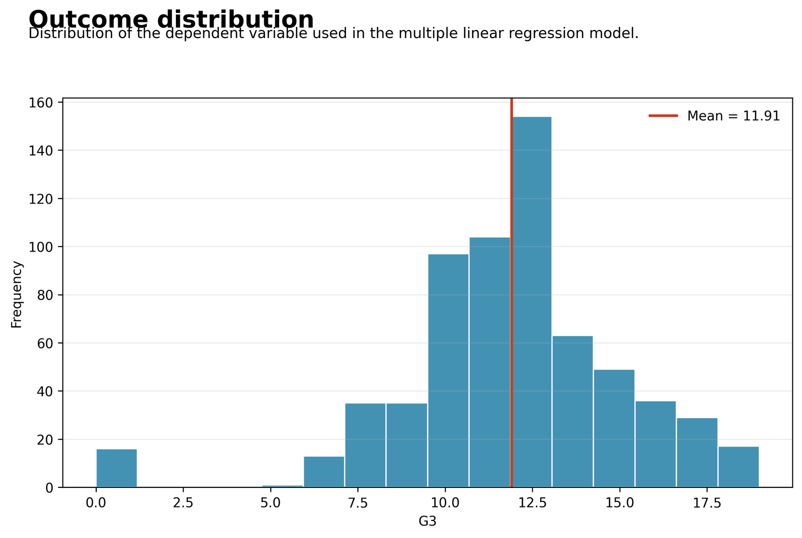
The histogram shows how final grades are distributed before the predictors are added. It helps a beginner understand the scale, center and unusual low-grade observations.
The model uses 649 students. G3 has mean approximately 11.906, standard deviation 3.231, and range 0–19.
Most grades lie near the middle of the scale, but a small zero-grade group creates a longer lower tail. Regression residuals therefore require careful inspection.
Review Histogram Interpretation, Descriptive Statistics and Normal Distribution.
Python Chart 2: Observed vs Predicted G3
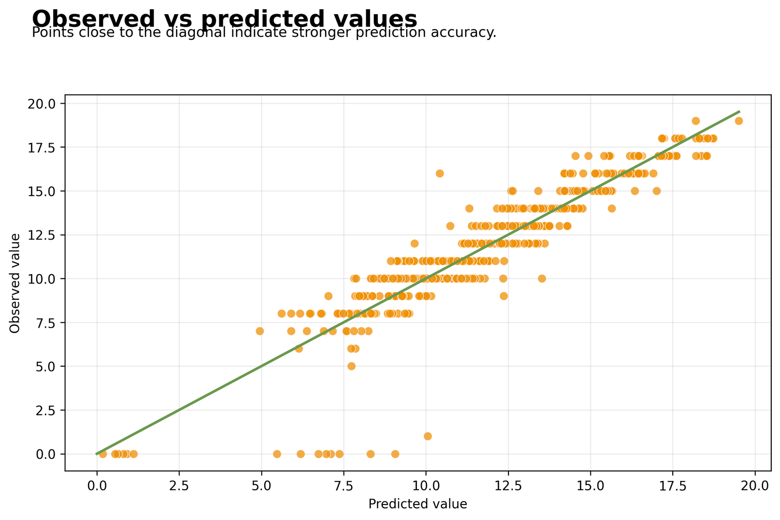
Points close to the diagonal line are predicted accurately. Horizontal bands appear because observed grades are integers while regression predictions are continuous.
Core-model R² = 0.8522, adjusted R² = 0.8501, RMSE = 1.2410, and MAE = 0.7799.
The equation explains about 85.22% of the observed variation in G3, but individual prediction errors can still be large for unusual students.
Use Adjusted R-Squared to understand fit after accounting for model size, then inspect residuals.
Python Chart 3: Residuals vs Predicted Values
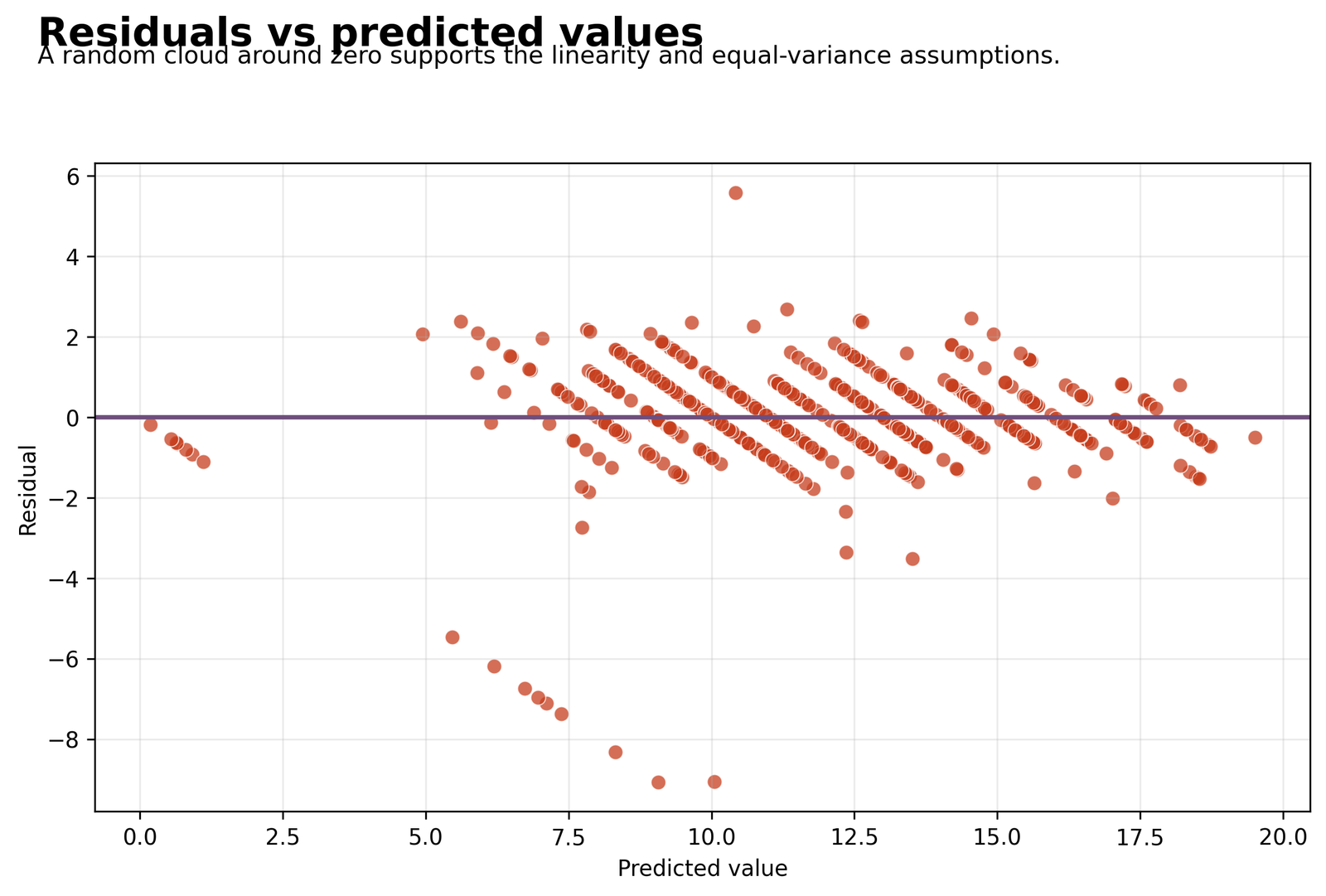
This plot checks whether errors remain centered around zero, whether they curve, and whether their spread changes across fitted values.
The core-model RMSE is 1.2410. In the expanded SPSS cross-check, residuals range from approximately -8.984 to +5.189.
Most predictions are close, but several unexpectedly low observed grades create a long negative residual tail. Those cases can affect normality and influence.
Use Studentized Residuals, Cook’s Distance and Influence Diagnostics.
Python Chart 4: Residual Distribution
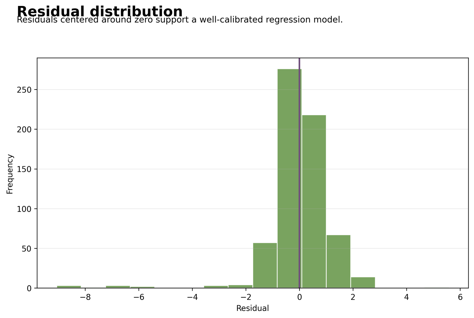
A good residual distribution is centered near zero. Long tails or strong asymmetry indicate that some observations are not well represented by the equation.
The Python core model reports Shapiro-Wilk p < .001. RMSE is 1.2410 and MAE is 0.7799.
The formal test rejects exact residual normality, largely because the sample is large and the negative tail contains difficult zero-grade cases.
Interpret the histogram with a Q-Q Plot, P-P Plot and Shapiro-Wilk Test.
Python Chart 5: Residual Q-Q Plot
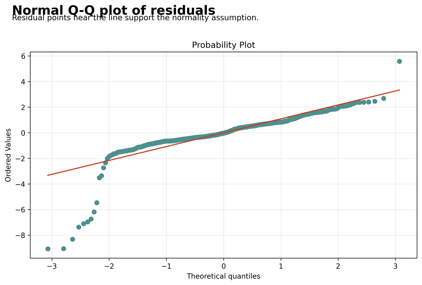
Points near the diagonal support approximate normality. Curvature at the ends indicates heavier or asymmetric residual tails.
Residual Shapiro-Wilk p-value is reported as 0.000000. The expanded SPSS residuals extend to about -8.984 and +5.189.
The central residuals may follow the line reasonably, while the lower tail departs because several observed grades are much lower than predicted.
Use the Skewness and Kurtosis guide and investigate unusual cases rather than deleting them automatically.
Python Chart 6: Multiple Linear Regression Coefficients
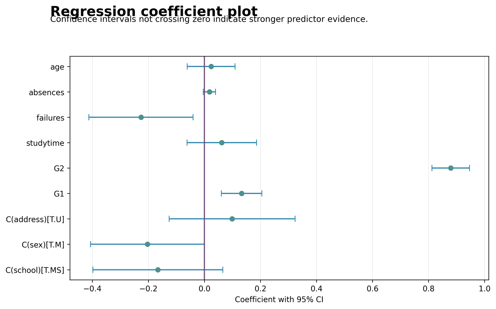
Each point is an unstandardized coefficient. The horizontal interval shows uncertainty. Intervals crossing zero indicate imprecise evidence at the 5% level.
G2 = 0.8794, G1 = 0.1328, failures = -0.2266, sex_M = -0.2037, school_MS = -0.1665, address_U = 0.0989, studytime = 0.0619, absences = 0.0177 and age = 0.0236.
G2 is the dominant predictor after all other core terms are controlled. G1, failures and sex_M also have intervals excluding zero in the core specification.
Read Partial Correlation and Semi-Partial Correlation to understand conditional predictor contributions.
Python Chart 7: Multiple Linear Regression Model Fit
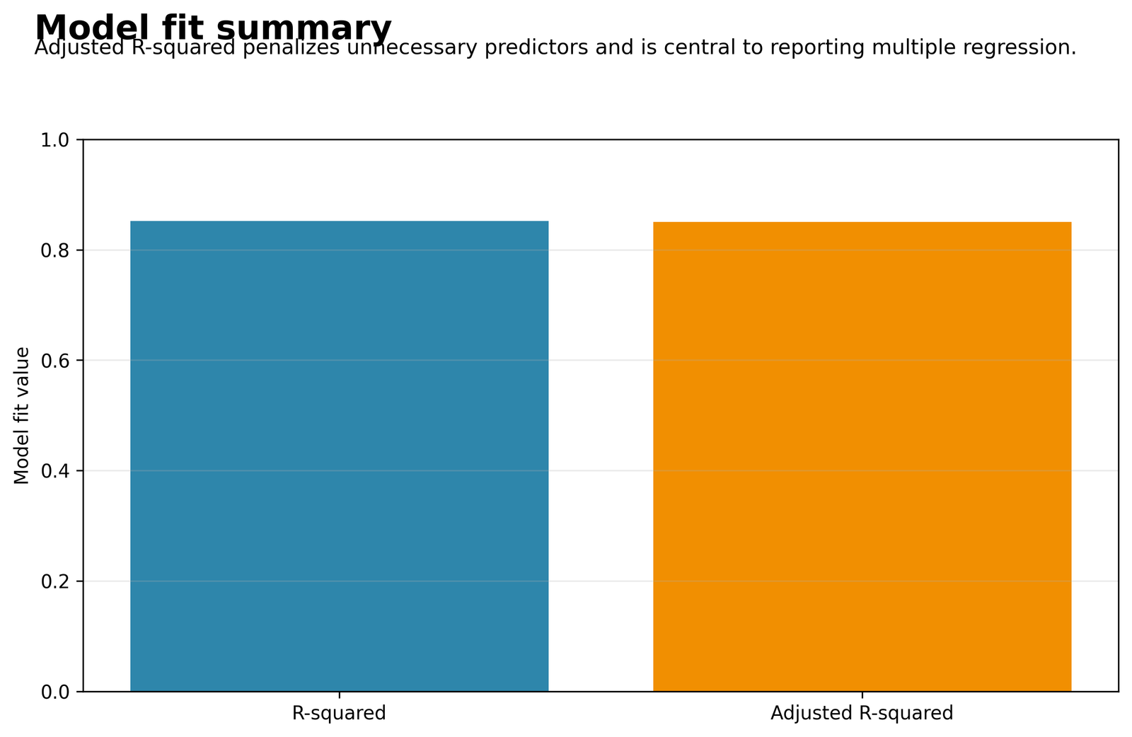
The figure combines the main statistics needed to judge whether the complete equation improves on predicting every student with the mean G3.
R² = 0.8522, adjusted R² = 0.8501, F(9,639) = 409.4514, p < .001, RMSE = 1.2410, MAE = 0.7799.
The complete core equation is highly significant and explains a large proportion of G3 variance. Adjusted R² is only slightly lower, showing that the nine slopes add substantial information.
Use P-Value, Effect Size and Adjusted R-Squared together.
Python Chart 8: Observed and Predicted G3 by G2
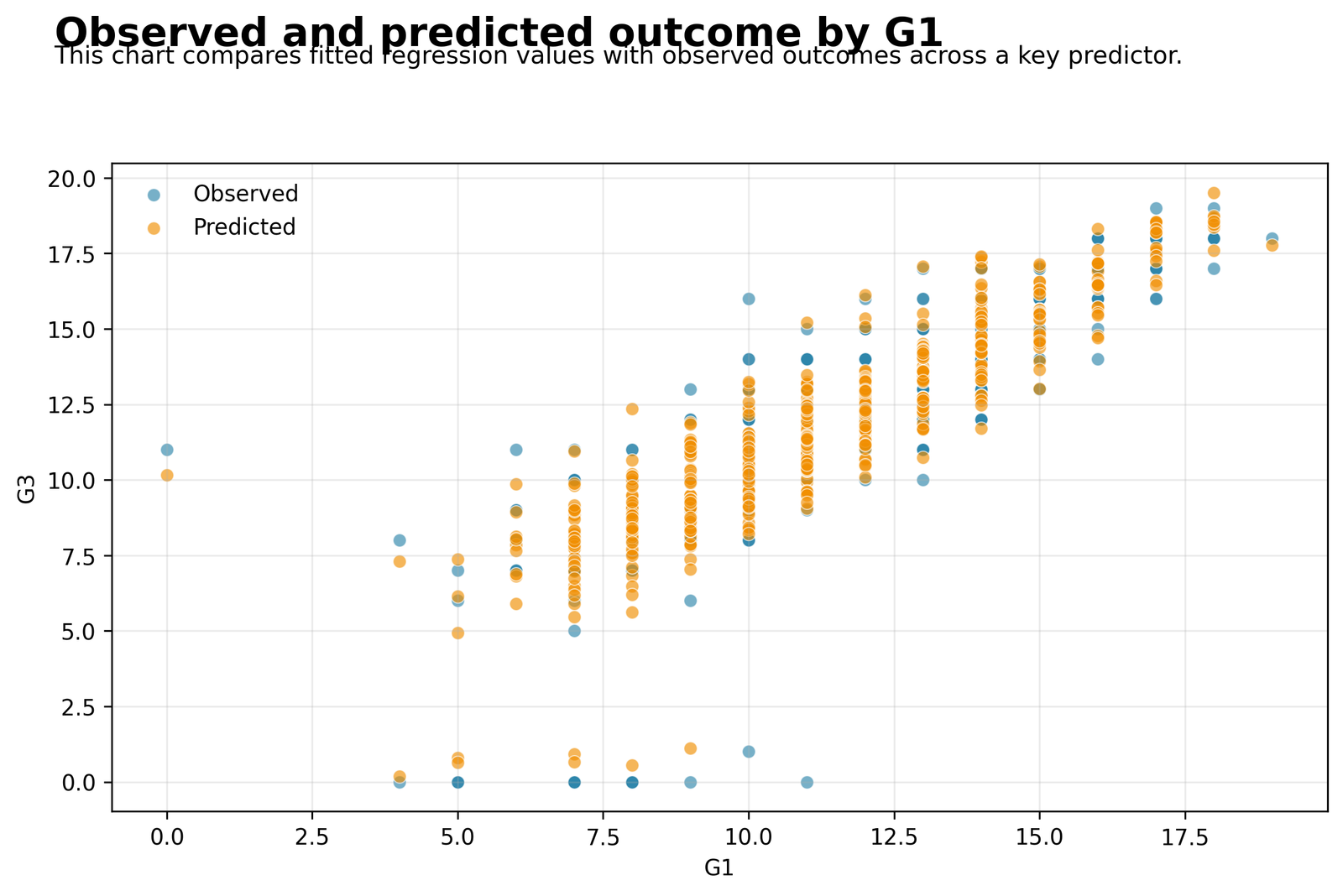
The chart shows why G2 dominates the equation. As G2 increases, both observed and predicted final grades rise strongly.
The G2 coefficient is 0.8794, 95% CI [0.8124, 0.9465], p < .001. The simple G2–G3 Pearson correlation is approximately 0.919.
Holding the other core predictors constant, one additional G2 point is associated with approximately 0.879 additional G3 points.
Compare the simple relationship in Pearson Correlation with the adjusted coefficient and review G1/G2 collinearity.
Open the complete Python Multiple Linear Regression report PDF
R Multiple Linear Regression Analytical Visuals in Paired Layout
The R section uses transparent HTML analytical panels rather than duplicating the hosted Python charts. When the same rows, references and formula are used, R’s lm() reproduces the ordinary least-squares core estimates.
R core formula
Core model metrics
R Visual 1: Core Regression Equation
G3 is predicted from G1, G2, studytime, failures, absences, age, school, sex and address.
R Visual 2: Core Model Fit
R² = 0.8522, adjusted R² = 0.8501, F = 409.4514, RMSE = 1.2410, MAE = 0.7799.
Explained variance
SPSS model comparison
R Visual 3: Core versus Expanded Fit
Core R² = 0.8522; expanded R² = 0.8541; expanded adjusted R² = 0.8507.
R Visual 4: G1 and G2 versus Additional Predictors
G1+G2 R² = 0.848; additional 13 terms add ΔR² = 0.006, F-change = 2.125, p = .011.
Selected coefficient magnitudes
Collinearity diagnostics
R Visual 5: Significant Coefficients
G2 about +0.88; G1 about +0.133; failures about -0.22; sex_M -0.204 in the core model; traveltime +0.143 in the expanded model.
R Visual 6: VIF and Tolerance
G1 VIF = 4.2214, tolerance = 0.2369; G2 VIF = 4.1019, tolerance = 0.2438.
Mean-profile prediction
Expanded-model ANOVA
R Visual 7: Worked Prediction at Mean Inputs
Predicted G3 = 11.9060, matching the observed mean input of approximately 11.9060.
R Visual 8: Residual and ANOVA Summary
Expanded SSE = 986.5652, SSR = 5776.7014, SST = 6763.2666; residual df = 633.
Multiple Linear Regression Coefficients Explained
The core and expanded equations are displayed together so students can see which conclusions remain stable when six additional variables are added.
| Term | Python core B | Core p | SPSS/Excel B | Expanded p | Interpretation |
|---|---|---|---|---|---|
| Intercept | -0.2405 | .7573 | -0.5656 | .5023 | Not significant in either model |
| G1 | 0.1328 | .0003 | 0.1328 | .0003 | Significant positive predictor |
| G2 | 0.8794 | <.001 | 0.8757 | <.001 | Dominant positive predictor |
| studytime | 0.0619 | .3283 | 0.0545 | .3910 | Not significant |
| failures | -0.2266 | .0170 | -0.2186 | .0227 | Significant negative predictor |
| absences | 0.0177 | .1133 | 0.0163 | .1464 | Not significant |
| age | 0.0236 | .5872 | 0.0314 | .4788 | Not significant |
| school_MS | -0.1665 | .1590 | -0.2059 | .0889 | Negative but imprecise |
| sex_M / sex_male | -0.2037 | .0493 | -0.1911 | .0709 | Significant only in core model |
| address_U / address_urban | 0.0989 | .3881 | 0.1639 | .1700 | Not significant |
| Medu | Not included | — | -0.0470 | .4324 | Not significant in expanded model |
| Fedu | Not included | — | 0.0265 | .6542 | Not significant in expanded model |
| traveltime | Not included | — | 0.1435 | .0489 | Small significant positive coefficient |
| health | Not included | — | -0.0485 | .1622 | Not significant |
| higher_yes | Not included | — | 0.1891 | .2919 | Not significant |
| internet_yes | Not included | — | 0.0700 | .5726 | Not significant |
G2: the dominant predictor
G2 is approximately 0.88 in both models. Its standardized SPSS beta is 0.790 in the expanded equation. This shows that second-period grade contributes much more conditional information than any other predictor.
G1: a smaller independent prior-grade effect
G1 remains approximately 0.133 after G2 is controlled. Because G1 and G2 are strongly correlated, the G1 slope represents the part of earlier achievement that is not already represented by G2.
Failures: a stable negative predictor
The failures coefficient is about -0.22 in both specifications. One additional previous failure is associated with approximately 0.22 lower G3 points after the remaining variables are controlled.
Why significance can change
The sex coefficient has p = .0493 in the core model but p = .0709 in the expanded model. Adding correlated or explanatory variables can change a coefficient and its standard error. A small change around the .05 boundary should be described transparently rather than treated as a completely different scientific story.
Core Predictors versus the Expanded Multiple Linear Regression Model
SPSS provides an especially useful comparison. A model containing only G1 and G2 explains 84.8% of G3 variance. Adding thirteen student-background and behavior terms raises R² to 85.4%.
G1 and G2 model
- R² = 0.848
- Adjusted R² = 0.847
- F = 1798.671
- Std. error of estimate = 1.262
Expanded fifteen-slope model
- R² = 0.854
- Adjusted R² = 0.851
- ΔR² = 0.006
- F-change(13,633) = 2.125, p = .011
The added block is statistically significant, but its practical contribution is small because prior grades already explain most of the outcome variance. Statistical significance and practical importance are therefore not the same.
Use Adjusted R-Squared to compare models with different predictor counts and Effect Size to discuss the magnitude of the incremental improvement.
Multiple Linear Regression Assumptions and Diagnostics
Beginner idea: a high R² does not prove that every assumption is satisfied. Diagnostics check whether the equation’s form, residual behavior and coefficient stability are reasonable.
Main assumptions
- G3 is continuous.
- Observations are independent.
- Relationships are reasonably linear.
- Residual variance is reasonably stable.
- Predictors are not destructively collinear.
- No few observations dominate the equation.
Current evidence
- Residual Shapiro-Wilk p < .001.
- G1 VIF = 4.2214.
- G2 VIF = 4.1019.
- Other core VIF values are near 1.07–1.31.
- Expanded residuals range about -8.984 to +5.189.
- Large negative residuals require review.
Linearity and specification
Use residual-versus-fitted patterns and the Ramsey RESET Test to look for omitted nonlinear structure. A straight-line coefficient may be inadequate near grade ceilings or floors.
Homoscedasticity
Use the Breusch-Pagan Test and White Test to check whether residual variance changes with fitted values or predictor combinations.
Residual normality
The Shapiro-Wilk test rejects exact normality. Use the Q-Q Plot, P-P Plot and Skewness and Kurtosis to judge how serious the departure is.
Multicollinearity
G1 and G2 have the largest VIF values because both measure prior achievement. Review the Multicollinearity Check, Variance Inflation Factor and Tolerance Statistic.
Outliers and influence
Use Studentized Residuals, Cook’s Distance, Mahalanobis Distance and Influence Diagnostics.
Independence
For ordered or time-based data, the Durbin-Watson Test can assess first-order residual autocorrelation. For cross-sectional students, independence should primarily follow from the sampling design.
Multiple Linear Regression in Python, R, SPSS and Excel
Python Multiple Linear Regression
Use statsmodels OLS with a formula and categorical coding. New users can begin with Correlation in Python.
- Core nine-slope formula
- ANOVA and coefficients
- VIF diagnostics
- Eight charts
R Multiple Linear Regression
Use lm(), anova(), confint() and VIF functions. New users can begin with Correlation in R.
- Factor-reference control
- Coefficient and ANOVA tables
- Residual plots
- Model comparison
SPSS Multiple Linear Regression
Use Analyze → Regression → Linear. Request coefficients, ANOVA, confidence intervals, collinearity statistics and residual plots. New users can begin with Correlation in SPSS.
- Expanded fifteen-slope model
- Core-versus-expanded change statistics
- Predicted and residual variables
- SPSS PDF output
Excel Multiple Linear Regression
Use the Data Analysis Regression tool or imported coefficient results. New users can begin with Correlation in Excel.
- Dashboard
- Coefficient table
- Model-fit formulas
- Prediction calculator
Multiple Linear Regression Worked Excel File Explained
The workbook contains Dashboard, Coefficients, Model_Fit, Prediction_Calculator and Worked_Data_Sample sheets. It reports the expanded fifteen-slope equation and provides formula-based checks.
Dashboard
The Dashboard reports 649 rows, R² = 0.8541289, adjusted R² = 0.8506722, RMSE = 1.2329360 and an overall model p-value below the worksheet’s displayed precision.
Model_Fit sheet
SSE is 986.5652, SSR is 5776.7014 and SST is 6763.2666. The F statistic is 247.0965 with 15 regression degrees of freedom and 633 residual degrees of freedom.
Prediction Calculator
The calculator multiplies each input by its coefficient and adds every contribution. With mean predictor inputs and average dummy proportions, predicted G3 equals approximately 11.9060, matching the observed outcome mean.
This identity occurs because ordinary least squares with an intercept has mean residual equal to zero. The workbook also calculates residual, squared residual and absolute residual for a user-entered profile.
Why Excel RMSE and SPSS standard error differ
The workbook calculates RMSE as √(SSE/N), producing 1.2329. SPSS reports the standard error of the estimate as √(SSE/residual df), producing approximately 1.248. Both use the same SSE but divide by different denominators.
Multiple Linear Regression Code: Expand the Software You Need
Python core model code
import pandas as pd
import statsmodels.formula.api as smf

df = pd.read_csv("dataset.csv")

formula = (
    "G3 ~ G1 + G2 + studytime + failures + absences + age"
    " + C(school) + C(sex) + C(address)"
)

model = smf.ols(formula, data=df).fit()

print(model.summary())
print(model.conf_int())

df["predicted_G3"] = model.fittedvalues
df["residual_G3"] = model.resid
Python VIF code
import pandas as pd
from patsy import dmatrix
from statsmodels.stats.outliers_influence import variance_inflation_factor

X = dmatrix(
    "G1 + G2 + studytime + failures + absences + age"
    " + C(school) + C(sex) + C(address)",
    data=df,
    return_type="dataframe",
)

X_no_intercept = X.drop(columns=["Intercept"])

vif = pd.DataFrame({
    "term": X_no_intercept.columns,
    "vif": [
        variance_inflation_factor(X_no_intercept.values, i)
        for i in range(X_no_intercept.shape[1])
    ],
})

vif["tolerance"] = 1 / vif["vif"]
print(vif)
R core and expanded models
df <- read.csv("dataset.csv", stringsAsFactors = TRUE)

core <- lm(
  G3 ~ G1 + G2 + studytime + failures + absences +
    age + school + sex + address,
  data = df
)

expanded <- lm(
  G3 ~ G1 + G2 + studytime + failures + absences +
    age + Medu + Fedu + traveltime + health +
    school + sex + address + higher + internet,
  data = df
)

summary(core)
confint(core)
anova(core)
summary(expanded)
anova(core, expanded)
SPSS expanded-model syntax
REGRESSION
 /MISSING LISTWISE
 /STATISTICS COEFF OUTS R ANOVA COLLIN CI(95) ZPP
 /CRITERIA=PIN(.05) POUT(.10) TOLERANCE(.0001)
 /NOORIGIN
 /DEPENDENT G3
 /METHOD=ENTER G1 G2 studytime failures absences age
   Medu Fedu traveltime health school_ms sex_male
   address_urban higher_yes internet_yes
 /SAVE PRED(Predicted_G3) RESID(Residual_G3)
       ZPRED(ZPred_G3) ZRESID(ZResid_G3).

OUTPUT SAVE
 /OUTFILE='D:\DATA ANALYSIS\H Regression Tests and Models\Multiple Linear Regression\SPSS_Output\spv\Multiple-Linear-Regression.spv'.

OUTPUT EXPORT
 /CONTENTS EXPORT=ALL LAYERS=PRINTSETTING MODELVIEWS=PRINTSETTING
 /PDF DOCUMENTFILE='D:\DATA ANALYSIS\H Regression Tests and Models\Multiple Linear Regression\SPSS_Output\pdf\Multiple-Linear-Regression-SPSS-Output.pdf'.
Excel formulas
Predicted G3:
=Intercept
 + G1*Beta_G1
 + G2*Beta_G2
 + Studytime*Beta_Studytime
 + Failures*Beta_Failures
 + Absences*Beta_Absences
 + Age*Beta_Age
 + Other_Predictor_Contributions

Residual:
=Observed_G3-Predicted_G3

Squared residual:
=Residual^2

R squared:
=1-SSE/SST

Adjusted R squared:
=1-(1-R2)*(N-1)/(N-k)

F statistic:
=(SSR/(k-1))/(SSE/(N-k))

RMSE:
=SQRT(SSE/N)

MAE:
=AVERAGE(Absolute_Residual_Range)
How a New Student Should Study This Multiple Linear Regression Example
- Identify Y: G3 is the outcome.
- Identify the predictors: G1, G2 and the control variables are X variables.
- Read R²: the core equation explains 85.22% of G3 variance.
- Read the overall F test: the complete predictor set improves on the mean-only model.
- Read G2 first: it is the strongest adjusted predictor.
- Read every coefficient conditionally: hold the other predictors constant.
- Check VIF: G1 and G2 overlap strongly but remain within the reported acceptable range.
- Check residuals: high R² does not remove outliers or tail departures.
- Compare specifications: do not mix the core and expanded equations.
- Write a balanced conclusion: report fit, coefficients, uncertainty and diagnostics.
Before moving to advanced material, explain the analysis without formulas: the model predicts final grade from several variables, gives each predictor an adjusted coefficient, and checks how close the predictions are to the observed grades.
Review Descriptive Statistics, Standard Error, Confidence Interval and Null and Alternative Hypothesis.
Advanced Multiple Linear Regression Interpretation and Extensions
The main reading path remains beginner-friendly. Expand only the technical topic needed for the study.
Why the intercept is not significant
- The intercept represents a combination of zeros and reference categories.
- That profile is not substantively typical for prior grades and age.
- A non-significant intercept does not weaken the predictor conclusions.
Why a coefficient can change sign
- A simple relationship can differ after other predictors enter.
- Shared variance and suppression can change direction.
- Always compare simple correlations with adjusted slopes carefully.
Suppression effects
- A suppressor can improve prediction by controlling irrelevant variance.
- Its coefficient may look surprising relative to its simple correlation.
- Theory and diagnostics should guide interpretation.
Standard error of a coefficient
- Standard error measures sampling uncertainty around B.
- It depends on residual variance, sample size and collinearity.
- The t statistic equals B divided by its standard error.
Confidence interval interpretation
- An interval gives plausible coefficient values under the model.
- Intervals crossing zero correspond to p-values above .05 in two-sided tests.
- Interval width shows precision.
Overall F test versus individual t tests
- The F test evaluates whether all slopes are zero jointly.
- Individual t tests evaluate one coefficient at a time.
- A significant model can contain several non-significant slopes.
Reference coding and intercept changes
- Changing reference categories alters the intercept and categorical contrasts.
- Fitted predictions and R² remain unchanged.
- Name every reference category in the report.
Prediction for a new student
- Insert the student’s values into the equation.
- Apply the same dummy coding used during fitting.
- Use a prediction interval to show individual uncertainty.
Extrapolation
- Predictions outside the observed predictor ranges are less trustworthy.
- A linear equation may continue beyond realistic grade boundaries.
- State the ranges used to fit the model.
Influence of zero grades
- Zero G3 observations produce some of the largest negative residuals.
- They can be valid academic outcomes.
- Sensitivity analysis should be reported if they strongly affect coefficients.
Robust regression sensitivity
- Robust regression reduces the effect of extreme residuals.
- It answers a slightly different estimation question.
- Compare directions and conclusions rather than expecting identical coefficients.
Transformation decisions
- Transformations can address nonlinearity or unequal variance.
- A transformed outcome changes coefficient interpretation.
- Use transformations only when diagnostics and subject matter support them.
Categorizing continuous predictors
- Turning numeric variables into groups discards information.
- It can create artificial thresholds.
- Retain continuous scales unless a strong reason supports categories.
Adding many weak predictors
- Raw R² always increases or stays the same.
- Adjusted R² may decrease when the added information is insufficient.
- The SPSS change is statistically significant but practically small.
Replicating results across software
- Use identical rows, formulas and reference categories.
- Check whether software reports RMSE or residual standard error.
- Small rounding differences are expected.
Using the correlation matrix
- A correlation matrix summarizes pairwise linear relationships.
- It can identify strong predictor overlap before fitting.
- Use the Correlation Matrix and Correlation Heatmap guides.
Planning a future analysis
- Specify the smallest meaningful effect.
- Account for the number of tested predictors.
- Allow for collinearity when estimating power.
Type I and Type II errors
- A Type I error is a false positive.
- A Type II error is a missed real effect.
- Read Type I and Type II Error for the trade-off.
Practical versus statistical significance
- Large samples can make small effects statistically significant.
- A coefficient should be interpreted on the G3 scale.
- Prediction improvement and collection cost also matter.
Transparent model documentation
- Record why every predictor was selected.
- Preserve the exact formula and coding.
- Report both primary and sensitivity specifications.
Multiple Linear Regression versus simple regression
- Simple regression includes one predictor.
- The multiple model estimates each predictor after controlling the others.
- A simple slope can differ substantially from an adjusted slope.
Multiple Linear Regression versus correlation
- Correlation is symmetric and pairwise.
- Regression distinguishes outcome and predictors.
- A coefficient represents a conditional expected change.
Unstandardized versus standardized coefficients
- Unstandardized B values remain in original units.
- Standardized beta values help compare predictors measured on different scales.
- Standardized magnitude does not replace practical interpretation.
Why G2 dominates the model
- G2 occurs close to G3 in time and correlates about 0.919 with G3.
- Its adjusted coefficient remains near 0.88.
- Strong prediction does not automatically prove a causal effect.
Why G1 remains significant after G2
- G1 and G2 share substantial information.
- G1 still contributes a smaller unique component.
- Its coefficient is conditional on G2 and all controls.
Why failures remains significant
- The coefficient stays near -0.22 across both specifications.
- The interval remains below zero.
- The relationship is adjusted but not automatically causal.
Why sex significance changes
- Its p-value moves from .0493 to .0709.
- Additional variables change the coefficient covariance and uncertainty.
- Borderline significance should be reported without binary exaggeration.
Why traveltime becomes significant
- Traveltime appears only in the expanded model.
- Its estimate is 0.1435 with p = .0489.
- The small positive coefficient requires cautious substantive interpretation.
Dummy-variable coding
- A zero indicates the reference category.
- A one indicates the target category.
- Changing references changes displayed contrasts but not fitted values.
Centering continuous predictors
- Centering can make the intercept more meaningful.
- It does not change R² or fitted values.
- It can simplify interactions and polynomial terms.
Interactions
- An interaction asks whether one slope changes across another variable.
- Main effects must be retained with the product term.
- Interpret conditional effects rather than the product coefficient alone.
Polynomial terms
- Squared terms model curvature.
- Retain the linear term whenever a squared term is included.
- Use plots and theory to justify added complexity.
Model selection
- Automated selection can produce unstable coefficients and optimistic p-values.
- Theory-driven specifications are generally easier to defend.
- Validation should accompany predictive selection.
Cross-validation
- In-sample RMSE describes fitted error.
- Cross-validation estimates error on unseen cases.
- All preprocessing should occur inside training folds.
Train-test split
- A held-out test set should be untouched during model development.
- One split can be unusually easy or difficult.
- Repeated resampling gives a more stable assessment.
Out-of-range predictions
- Ordinary regression predictions are unbounded.
- The expanded SPSS model includes a predicted value slightly below zero.
- Bounded outcomes may require sensitivity analysis.
Heteroskedasticity-consistent standard errors
- Robust covariance estimates can protect inference when variance is not constant.
- They do not change fitted coefficients.
- They do not repair nonlinear or omitted-variable bias.
Bootstrapped coefficients
- Resampling can estimate empirical coefficient uncertainty.
- The full model must be refitted in every sample.
- Report the bootstrap method and number of samples.
Multicollinearity and prediction
- A model can predict well even when individual slopes are unstable.
- G1 and G2 VIF values exceed four.
- Interpret their coefficients as conditional contributions.
Tolerance
- Tolerance equals one divided by VIF.
- Small tolerance indicates that a predictor is strongly explained by the others.
- G1 and G2 have the smallest reported tolerance values.
Residual normality in large samples
- Formal tests detect small departures when N is large.
- Confidence intervals may still be reasonably robust.
- Tail observations and influence should be investigated.
Leverage
- Leverage measures how unusual a predictor profile is.
- High leverage does not necessarily mean a large residual.
- Influence combines leverage and residual size.
Cook’s distance
- Cook’s distance summarizes how fitted results change when one case is removed.
- Use it with leverage and studentized residuals.
- Investigate rather than delete automatically.
Prediction intervals
- A confidence interval estimates the mean G3 for a predictor profile.
- A prediction interval estimates one new student’s G3.
- Prediction intervals are wider because they include residual variation.
ANOVA decomposition
- SST equals SSR plus SSE when an intercept is included.
- The F test compares explained and unexplained mean squares.
- A significant F test does not mean every slope is significant.
R-squared limitations
- R² cannot decrease when predictors are added.
- It does not prove causality or assumption validity.
- Adjusted R² and validation provide important context.
Incremental R-squared
- SPSS shows that thirteen added terms contribute ΔR² = .006.
- The change is significant because the sample is large.
- The practical improvement remains small.
Sample size and power
- There are 649 complete cases.
- Power depends on predictor count, effect size and collinearity.
- Use Statistical Power for planning.
Missing data
- The reported models use complete cases.
- Listwise deletion can change the analyzed population.
- Imputation should preserve the outcome-predictor structure.
Causal interpretation
- Regression adjustment does not prove causation.
- Unmeasured confounding and measurement error remain possible.
- Use causal language only with an appropriate design.
Reproducibility
- Save the formula, rows, coding and references.
- Record software and package versions.
- Export coefficients, predictions, residuals and diagnostic tables.
APA-Style Reporting for Multiple Linear Regression
Multiple Linear Regression Publication Checklist and Common Mistakes
Report these items
- Outcome and analyzed sample size
- Predictors and reference categories
- Model formula and specification
- R², adjusted R² and overall F test
- B, SE, t, p and confidence intervals
- RMSE and MAE with their denominator definitions
- VIF and tolerance
- Residual and influence diagnostics
- Validation method for prediction claims
- Software-specific differences
Avoid these mistakes
- Interpreting a coefficient without holding other predictors constant
- Calling a non-significant term completely unrelated
- Using R² as proof of causation
- Ignoring residual patterns because R² is high
- Mixing coefficients from different model specifications
- Confusing RMSE with SPSS standard error of estimate
- Ignoring dummy-variable references
- Deleting outliers only to improve significance
- Reporting p = .000 instead of p < .001
- Claiming in-sample error is future performance
Multiple Linear Regression Downloads
SPSS Multiple Linear Regression OutputExpanded model, model comparison, coefficients and residual diagnostics.
Multiple Linear Regression Worked Excel FileDashboard, coefficients, model-fit formulas and prediction calculator.
Adjusted R-Squared GuideContinue learning how predictor count affects model comparison.
Frequently Asked Questions About Multiple Linear Regression
What is Multiple Linear Regression?
Multiple Linear Regression predicts one continuous outcome from two or more predictors.
What is the outcome in this example?
G3 is the final-grade outcome.
How many observations are used?
The models use 649 complete student records.
How many predictors are in the Python core model?
The Python core equation has nine slopes.
How many predictors are in the SPSS and Excel expanded model?
The expanded equation has fifteen slopes plus an intercept.
What is the Python core R-squared?
The core R² is 0.8522.
What is the expanded R-squared?
The SPSS and Excel expanded R² is approximately 0.8541.
What is adjusted R-squared?
It is an explained-variance measure that penalizes unnecessary predictors.
What is the strongest predictor?
G2 is the strongest adjusted predictor.
What is the G2 coefficient?
It is 0.8794 in the Python core model and 0.8757 in the expanded model.
Is G1 still significant after G2 is included?
Yes. Its coefficient remains approximately 0.133.
Is failures significant?
Yes. Its coefficient is approximately -0.22 in both specifications.
Is studytime significant?
No. Its p-value exceeds .05 in both reported specifications.
Is sex significant?
It is just significant in the core model but not in the expanded model.
Is travel time significant?
It has p = .0489 in the expanded model.
What does holding predictors constant mean?
It means comparing cases with the same values on all other predictors.
What does R-squared mean?
It is the proportion of observed G3 variation explained by the fitted equation.
Does high R-squared prove causation?
No. It describes fit, not causal identification.
What is RMSE?
RMSE summarizes squared prediction error on the outcome scale.
What is MAE?
MAE is the average absolute difference between observed and predicted G3.
Why is Excel RMSE different from SPSS standard error?
They divide the same SSE by different denominators.
What is VIF?
VIF measures how much predictor overlap inflates coefficient variance.
What are the largest VIF values?
G1 is 4.2214 and G2 is 4.1019.
Are those VIF values severe?
They show noticeable overlap but are reported as acceptable in the Python output.
Why is residual normality rejected?
The large sample and several extreme negative residuals create detectable departures.
Can Excel run the analysis?
Yes, but the worked file is primarily for calculations, auditing and prediction.
Can SPSS run the analysis?
Yes. Use Analyze, Regression, Linear.
Can R run the analysis?
Yes. Use lm() with the same formula and factor references.
Can Python run the analysis?
Yes. Use statsmodels OLS and diagnostic tools.
How should the final result be reported?
Report specification, fit, coefficients, confidence intervals, diagnostics and prediction limits.
Final Multiple Linear Regression Conclusion
Multiple Linear Regression results are most trustworthy when fit, uncertainty, residuals and validation support the same conclusion.
Multiple Linear Regression coefficients are conditional effects and should never be read as simple two-variable relationships.
Multiple Linear Regression should be explained by naming the outcome, predictors, references, equation and diagnostic evidence.
Multiple Linear Regression model comparisons must use the same observations and clearly defined predictor sets.
Multiple Linear Regression results are most trustworthy when fit, uncertainty, residuals and validation support the same conclusion.
Multiple Linear Regression coefficients are conditional effects and should never be read as simple two-variable relationships.
Multiple Linear Regression should be explained by naming the outcome, predictors, references, equation and diagnostic evidence.
Multiple Linear Regression model comparisons must use the same observations and clearly defined predictor sets.
Multiple Linear Regression results are most trustworthy when fit, uncertainty, residuals and validation support the same conclusion.
Multiple Linear Regression coefficients are conditional effects and should never be read as simple two-variable relationships.
Multiple Linear Regression should be explained by naming the outcome, predictors, references, equation and diagnostic evidence.
Multiple Linear Regression model comparisons must use the same observations and clearly defined predictor sets.
Multiple Linear Regression results are most trustworthy when fit, uncertainty, residuals and validation support the same conclusion.
Multiple Linear Regression coefficients are conditional effects and should never be read as simple two-variable relationships.
Multiple Linear Regression should be explained by naming the outcome, predictors, references, equation and diagnostic evidence.
Beginner conclusion: final grade can be predicted accurately from several student variables, but G1 and especially G2 provide most of the useful information.
The Python core model explains 85.22% of G3 variation and has adjusted R² = 0.8501. G2, G1, failures and sex_M have p-values below .05 in that specification. Residual diagnostics show that a small number of unusually low final grades remain difficult to predict.
The SPSS and Excel expanded model explains 85.41% of variation. Adding thirteen terms beyond G1 and G2 produces a statistically significant but small ΔR² of 0.006. This shows why model fit, effect magnitude and parsimony should be discussed together.

