
Heteroscedasticity, Error Covariance, Inverse-Variance Weighting and Feasible GLS
Generalized Least Squares Regression: Interpretation, SPSS, Python, R and Excel Guide
Generalized Least Squares Regression extends ordinary least squares when regression errors do not have equal independent variance. This guide compares OLS, feasible GLS/WLS, diagonal-covariance GLS and GLSAR using G3 final grade as the outcome. It explains the covariance matrix, variance-model weights, Breusch–Pagan and White tests, Durbin–Watson, coefficients, nine Python charts, nine R validation discussions, the current SPSS export problem and a separate formula-driven Excel example.
Quick Answer: Generalized Least Squares Regression Result
The verified Python and R analyses use 649 complete observations. The outcome is G3. Numeric predictors are G1, G2, studytime, failures, absences, age and Medu. Categorical predictors are school, sex and address. The baseline OLS residuals show strong heteroscedasticity, so inverse estimated error-variance weights are used for feasible GLS.
In the Python report, OLS has R² = 0.8524 and adjusted R² = 0.8501. Feasible GLS/WLS has R² = 0.8695 and adjusted R² = 0.8674. Its AIC decreases from 2143.3400 to 2037.0053, and BIC decreases from 2192.5698 to 2086.2351. MAE improves from 0.7791 to 0.7721, while unweighted RMSE changes slightly from 1.2403 to 1.2423.
Main conclusion: Breusch–Pagan and White diagnostics reject constant OLS error variance. Feasible GLS produces a substantially larger weighted R² and lower within-model AIC/BIC, while modestly improving MAE. The correction is motivated by heteroscedasticity, not strong serial correlation, because Durbin–Watson is close to 2 and the GLSAR AR(1) estimate is only 0.0661.
Important fit-metric caution: weighted and unweighted R², likelihood values and residual-error summaries are not always directly comparable across OLS and WLS/GLS. The FGLS weighted R² improvement is meaningful for the weighted objective, but the slight increase in unweighted RMSE shows that GLS does not uniformly improve every prediction metric.
SPSS status: the supplied SPSS PDF is not a completed GLS analysis. It contains only the warning “EMBEDBOOKMARKS is not a recognized subcommand” and says execution stopped. The SPSS output must be regenerated with the compatibility-safe PDF export command before coefficient tables can be reported.
Table of Contents
- What Is Generalized Least Squares Regression?
- Why OLS Can Be Inefficient
- GLS Matrix Formula
- Feasible GLS and Variance Modelling
- GLS vs WLS vs FGLS vs GLSAR
- When to Use Generalized Least Squares
- Dataset and Variables Used
- OLS Diagnostic Results
- OLS, FGLS, Diagonal GLS and GLSAR Comparison
- Coefficient Interpretation
- How GLS Weights Work
- GLS Assumptions
- Python Chart-by-Chart Interpretation
- R Charts, Tables and Independent Validation
- SPSS Output Status and Corrected Workflow
- Excel Worked GLS Results
- Python, R, SPSS and Excel Workflows
- Generalized Least Squares Code
- GLS vs Robust Standard Errors
- Prediction, Fit and Model Selection
- APA-Style Reporting
- Reporting Checklist
- Common Mistakes
- Troubleshooting Guide
- Downloads and Resources
- Related Salar Cafe Guides
- FAQs
What Is Generalized Least Squares Regression?
Generalized Least Squares Regression is a linear regression estimator designed for errors with a non-spherical covariance structure. Ordinary least squares assumes that, conditional on the predictors, errors have equal variance and are uncorrelated. GLS allows error variances to differ and errors to be correlated according to a specified covariance matrix.
When the covariance matrix is known, GLS transforms the data so that the transformed errors satisfy the ordinary least-squares conditions. When the covariance structure is unknown and estimated from data, the method is called feasible generalized least squares.
Simple definition: GLS gives observations and residual patterns different influence according to the estimated error covariance, rather than treating every observation as equally precise.
What Changes from OLS?
GLS can change coefficient estimates, standard errors, confidence intervals, p-values and fitted values. It does not merely replace conventional standard errors. If the weighting or covariance model is correct, GLS can be more efficient than OLS. If it is misspecified, the apparent precision gain can be misleading.
Why Ordinary Least Squares Can Be Inefficient
Under heteroscedasticity, OLS coefficient estimates can remain unbiased when the conditional-mean model is correct, but ordinary OLS standard errors become unreliable and the estimator is no longer the most efficient linear unbiased estimator. High-variance observations receive the same influence as low-variance observations even though their outcomes are less precisely measured.
Under serial or clustered correlation, OLS also ignores dependence between errors. The effective information is smaller than the raw record count suggests. GLS addresses these problems by modelling a covariance matrix rather than assuming the identity matrix multiplied by one variance.
| Error Problem | OLS Consequence | GLS Response | Example |
|---|---|---|---|
| Heteroscedasticity | Incorrect conventional SEs and inefficient coefficients. | Use observation-specific inverse-variance weights. | Error spread increases with fitted G3. |
| AR(1) serial correlation | Residuals depend on the preceding observation. | Model off-diagonal covariance using ρ. | Time-series residuals persist over periods. |
| Cluster correlation | Within-cluster observations are not independent. | Specify block covariance or use mixed/panel methods. | Repeated students within schools. |
| Known measurement precision | All observations are treated equally. | Weight by known inverse measurement variance. | Study estimates with different standard errors. |
Generalized Least Squares Matrix Formula
The linear model is:
When Ω is known and positive definite, the GLS coefficient estimator is:
If Ω = σ²I, the formula reduces to OLS. If Ω is diagonal with observation-specific variances, GLS becomes weighted least squares. If Ω contains off-diagonal correlations, GLS also accounts for error dependence.
Whitening Transformation
Suppose a matrix P satisfies P′P = Ω⁻¹. Multiplying the model by P produces transformed errors with identity covariance:
OLS applied to the transformed outcome and predictors produces the GLS estimator. This interpretation helps explain why GLS is still a least-squares method: it minimizes squared residuals in transformed space.
Feasible Generalized Least Squares and the Variance Model
The complete covariance matrix is rarely known. Feasible GLS first fits OLS, uses OLS residuals to estimate the error-variance pattern, constructs an estimated covariance matrix and then refits the regression using that estimate.
Worked Analysis Variance Model
The predicted log variance is exponentiated to obtain a positive estimated variance. The feasible GLS weight is:
Observations with smaller predicted error variance receive larger weights. Observations with larger predicted variance receive smaller weights. The full-data weight distribution spans approximately 1.9 to 5.1 in the supplied histogram, with the greatest concentration around 2.7 to 3.4.
Why Log Residual Squared?
Squared residuals are nonnegative and highly skewed. Modelling their logarithm ensures that exponentiated predictions are positive and can stabilize the variance relationship. A small constant prevents taking the logarithm of zero.
One-Step vs Iterated FGLS
The supplied workflow is a practical one-step FGLS correction: OLS residuals estimate variance, and the weighted model is fitted once. Iterated FGLS repeats variance estimation and weighting until convergence. Iteration may improve internal consistency but can also amplify a misspecified variance model.
GLS vs WLS vs FGLS vs GLSAR
| Method | Covariance Structure | Weights / Parameters | Use in This Analysis |
|---|---|---|---|
| OLS | σ²I | All observations have equal weight. | Baseline model and source of diagnostic residuals. |
| WLS | Diagonal Ω | Known or supplied weights. | Computational form used for feasible inverse-variance weights. |
| FGLS | Estimated Ω | Weights estimated from OLS residual variance. | Main model. |
| Diagonal GLS | Estimated diagonal covariance matrix | σ̂ᵢ² on the diagonal. | Numerically validates the FGLS/WLS fit. |
| GLSAR | AR(p) covariance | ρ estimated iteratively. | Autocorrelation comparison; ρ = 0.0661. |
The feasible WLS and diagonal GLS models produce nearly identical results: Python R² = 0.8695, adjusted R² = 0.8674 and MAE = 0.7721 for both. Their AIC values differ only from 2037.0053 to 2037.0021 because the implementations represent the same diagonal covariance correction.
When to Use Generalized Least Squares Regression
| Situation | Use GLS? | Reason |
|---|---|---|
| OLS residual variance changes systematically | Possibly | FGLS can model the variance and improve efficiency. |
| Known observation variances | Yes | Inverse known variance is a principled weight. |
| Time-series errors follow AR(1) | Use GLSAR or time-series GLS | Off-diagonal covariance matters. |
| Only standard errors are heteroscedastic but coefficients are the main target | Robust OLS may be preferable | It avoids specifying a variance model. |
| Weights are arbitrary importance scores | No | GLS weights should represent error precision, not subjective importance. |
| Outcome is nonnormal or bounded and mean-variance relation is intrinsic | Consider GLM | A generalized linear model may match the outcome distribution better. |
| Repeated observations within clusters | Consider GEE/mixed models | Correlation structure and subject-level interpretation may require another framework. |
The decision should begin with the error structure and research goal, not with a desire to obtain a larger R² or smaller p-value.
Dataset and Variables Used
The Python and R reports use the same 649 complete observations and the same formula. G3 is the continuous outcome. Seven numeric predictors and three categorical predictors enter both OLS and FGLS.
Variable Dictionary
| Variable | Role | Meaning / Coding | Coefficient Interpretation |
|---|---|---|---|
| G3 | Outcome | Final grade from 0 to 19. | Predicted final-grade points. |
| G1 | Numeric predictor | First-period grade. | Expected G3 change for one higher G1 point. |
| G2 | Numeric predictor | Second-period grade. | Expected G3 change for one higher G2 point. |
| studytime | Numeric predictor | Weekly study-time category. | Expected G3 change for one higher category. |
| failures | Numeric predictor | Previous class failures. | Expected G3 change for one additional failure. |
| absences | Numeric predictor | School absence count. | Expected G3 change for one additional absence. |
| age | Numeric predictor | Student age. | Expected G3 change for one additional year. |
| Medu | Numeric predictor | Mother’s education level. | Expected G3 change for one higher education level. |
| school_MS | Dummy predictor | 1 = MS; 0 = GP reference. | Adjusted MS versus GP difference. |
| sex_M | Dummy predictor | 1 = M; 0 = F reference. | Adjusted M versus F difference. |
| address_U | Dummy predictor | 1 = urban; 0 = rural reference. | Adjusted urban versus rural difference. |
Error-Variance Variables
OLS fitted values, OLS residuals, squared residuals, predicted log variance, estimated variance and inverse estimated variance weights are derived quantities. They are not substantive predictors in the main G3 equation; they define the FGLS covariance correction.
OLS Diagnostic Results That Motivate GLS
| Diagnostic | Python Statistic | Python p-value | R Statistic | R p-value | Interpretation |
|---|---|---|---|---|---|
| Breusch–Pagan LM | 34.4086 | 0.000157 | 19.0968 | 0.0000124 | Strong evidence of nonconstant variance. |
| Breusch–Pagan F | 3.5719 | 0.0001 | Not separately reported | — | Supports the same heteroscedasticity conclusion. |
| White LM | 106.8797 | 0.000348 | 20.0366 | 0.0000446 | General heteroscedasticity pattern is present. |
| White F | 1.8634 | 0.0001 | Not separately reported | — | Supports rejection of constant variance. |
| Durbin–Watson | 1.8723 | Not applicable | 1.8723 | Not applicable | Close to 2; weak first-order residual dependence. |
| Jarque–Bera | 9864.1705 | < .001 | 9795.7819 | < .001 | Residuals strongly deviate from normality. |
Python and R use somewhat different auxiliary-test implementations, so the exact Breusch–Pagan and White statistics differ. Both software packages produce the same decision: heteroscedasticity is statistically clear. The Durbin–Watson statistic and GLSAR estimate show that serial dependence is not the principal problem.
Normality context: Jarque–Bera significance is not the reason for using GLS. GLS corrects the covariance structure. Residual nonnormality may still affect small-sample inference and tail prediction, but it is a separate issue.
OLS, Feasible GLS, Diagonal GLS and GLSAR Model Comparison
Python Model Comparison
| Model | N | df Model | df Residual | R² | Adjusted R² | AIC | BIC | RMSE | MAE | DW |
|---|---|---|---|---|---|---|---|---|---|---|
| OLS baseline | 649 | 10 | 638 | 0.8524 | 0.8501 | 2143.3400 | 2192.5698 | 1.2403 | 0.7791 | 1.8723 |
| Feasible GLS / WLS | 649 | 10 | 638 | 0.8695 | 0.8674 | 2037.0053 | 2086.2351 | 1.2423 | 0.7721 | 1.8716 |
| GLS diagonal covariance | 649 | 10 | 638 | 0.8695 | 0.8674 | 2037.0021 | 2086.2318 | 1.2423 | 0.7721 | 1.8716 |
| GLSAR AR(1) comparison | 649 | 10 | 637 | 0.8500 | 0.8477 | 2137.7207 | 2186.9335 | 1.2405 | 0.7786 | 1.8668 |
Feasible WLS and diagonal GLS are numerically equivalent for the estimated diagonal covariance matrix. Their weighted R² exceeds OLS by approximately 0.0171. MAE improves by 0.0070, but RMSE increases by 0.0020. The results therefore support the variance correction without claiming that every unweighted error criterion improves.
R Model Comparison
R reproduces OLS R² = 0.8523746, adjusted R² = 0.8500607, RMSE = 1.240328 and MAE = 0.7790877. Feasible GLS/WLS has R² = 0.8694957, adjusted R² = 0.8674502, RMSE = 1.242313 and MAE = 0.7721485.
R reports AIC/BIC as 2145.340/2199.045 for OLS and 2039.003/2092.708 for FGLS. These differ from Python by additive likelihood-convention constants. Compare AIC and BIC within the same software, not across different likelihood definitions.
OLS and Feasible GLS Coefficient Interpretation
Exact OLS Coefficients from the Reports
| Term | OLS B | SE | t | p-value | 95% CI | Decision |
|---|---|---|---|---|---|---|
| Intercept | -0.1646 | 0.7837 | -0.2101 | 0.8337 | -1.7035 to 1.3742 | Not significant |
| school: MS vs GP | -0.1788 | 0.1191 | -1.5015 | 0.1337 | -0.4126 to 0.0550 | Not significant |
| sex: M vs F | -0.1917 | 0.1045 | -1.8349 | 0.0670 | -0.3969 to 0.0135 | Not significant |
| address: U vs R | 0.1082 | 0.1151 | 0.9402 | 0.3475 | -0.1178 to 0.3343 | Not significant |
| G1 | 0.1337 | 0.0368 | 3.6344 | 0.0003 | 0.0615 to 0.2060 | Significant positive |
| G2 | 0.8814 | 0.0342 | 25.7364 | < .001 | 0.8142 to 0.9487 | Significant positive |
| studytime | 0.0641 | 0.0633 | 1.0121 | 0.3119 | -0.0602 to 0.1884 | Not significant |
| failures | -0.2315 | 0.0950 | -2.4377 | 0.0151 | -0.4179 to -0.0450 | Significant negative |
| absences | 0.0177 | 0.0112 | 1.5882 | 0.1127 | -0.0042 to 0.0397 | Not significant |
| age | 0.0222 | 0.0436 | 0.5089 | 0.6110 | -0.0634 to 0.1078 | Not significant |
| Medu | -0.0379 | 0.0467 | -0.8112 | 0.4176 | -0.1297 to 0.0539 | Not significant |
FGLS Coefficient Changes Shown in Chart 6
The PDF coefficient table is truncated after the FGLS intercept, which is exactly -0.3473, SE = 0.7111, p = 0.6254, 95% CI [-1.7436, 1.0490]. The comparison chart displays the remaining plotted FGLS coefficients graphically. Approximate bar values are school_MS ≈ -0.15, sex_M ≈ -0.16, address_U ≈ 0.08, G1 ≈ 0.14, G2 ≈ 0.86, studytime ≈ 0.05, failures ≈ -0.29 and absences ≈ 0.01.
The substantive pattern remains stable: G2 is the dominant positive coefficient, G1 is positive, and failures is negative. Weighting changes the magnitudes modestly, particularly making the failures coefficient more negative. Exact FGLS coefficient reporting should use the generated CSV table rather than reverse-reading the bar chart.
Transparency rule: approximate values inferred from an unlabeled coefficient bar chart are identified as approximate. Do not present them as exact four-decimal software output.
How Generalized Least Squares Weights Work
The full model assigns larger weights to observations with smaller estimated error variance. A weight twice as large does not mean an observation is twice as important substantively. It means the fitted covariance model treats it as having greater conditional precision.
| Estimated Variance | Inverse Weight | Influence in FGLS |
|---|---|---|
| Small | Large | Observation contributes more to the weighted objective. |
| Moderate | Moderate | Observation receives typical influence. |
| Large | Small | Observation is down-weighted because its outcome is less precise. |
Weights should be normalized only when needed for interpretation or software stability. Multiplying every weight by the same constant does not change WLS coefficient estimates, although it may affect reported likelihood scales.
Weight Diagnostics
Inspect minimum, maximum, quantiles and relationships with fitted values and predictors. Extremely large weights can cause a few observations to dominate. Extremely small weights can effectively remove observations from coefficient estimation. Trimming weights changes the estimand and requires justification.
Generalized Least Squares Regression Assumptions
| Assumption | Meaning | Diagnostic | Risk if Violated |
|---|---|---|---|
| Correct conditional mean | E(y|X) is represented appropriately. | Residual patterns, theory, transformations and RESET. | Both OLS and GLS coefficients can be biased. |
| Exogeneity | E(ε|X) = 0. | Research design and temporal ordering. | GLS does not fix endogeneity. |
| Covariance model reasonably specified | Estimated Ω reflects the main variance/dependence pattern. | Post-GLS residual plots and sensitivity models. | Efficiency and standard errors may be misleading. |
| Positive weights / positive-definite Ω | The transformation is mathematically valid. | Check finite positive estimated variances and matrix eigenvalues. | Model cannot be fitted stably. |
| No perfect multicollinearity | Predictors are not exact combinations. | Multicollinearity check, VIF and tolerance. | Coefficients are unidentified. |
| Independent observations conditional on Ω | Remaining dependence is represented. | Study design, residual autocorrelation and clustering. | Uncertainty may remain understated. |
GLS does not require raw outcomes to be normally distributed for coefficient consistency. Normality is mainly relevant to exact finite-sample inference and predictive distribution assumptions.
Python Chart-by-Chart Interpretation with Real Values
Python Chart 1: G3 Outcome Distribution
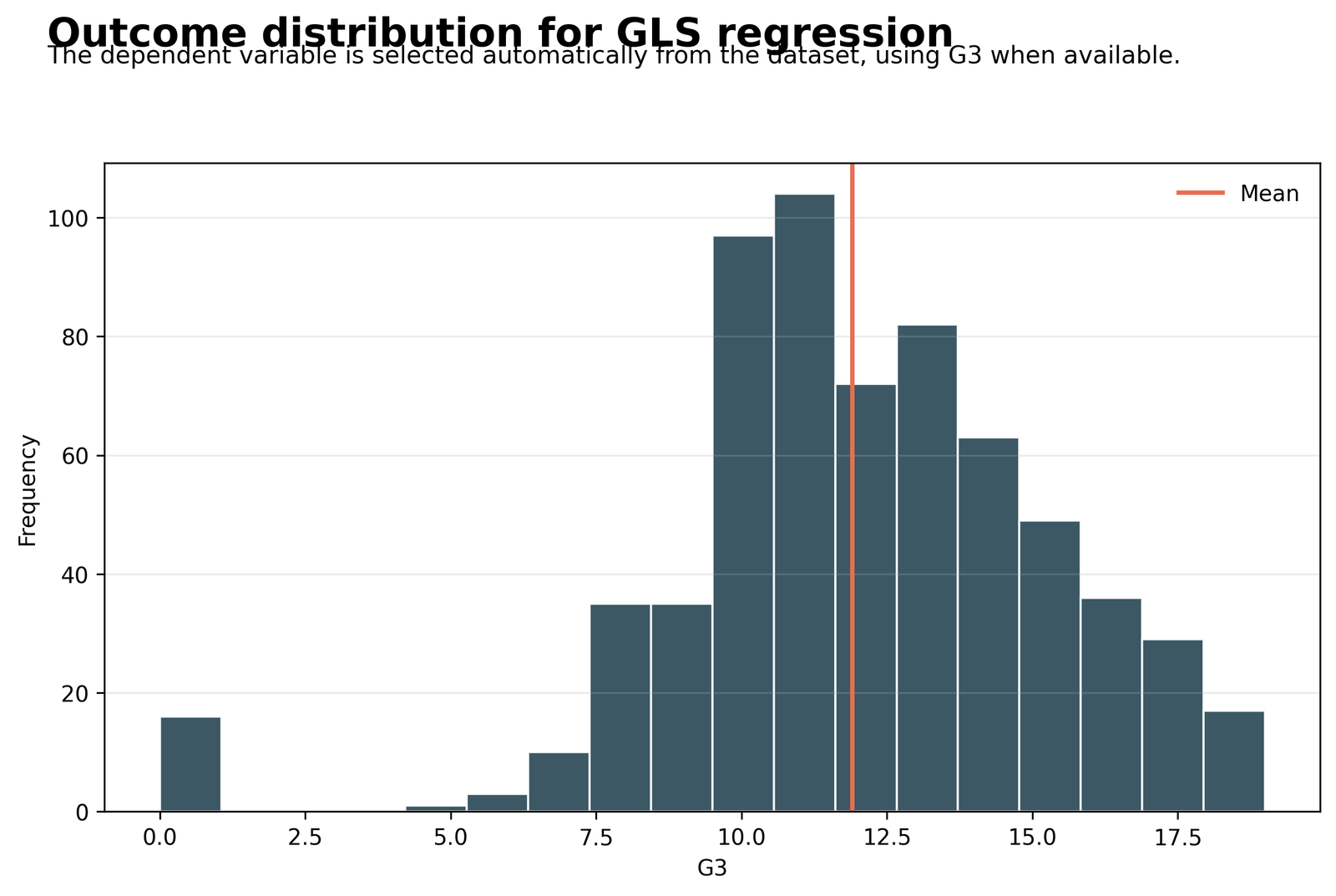
The analysis uses 649 G3 observations. The distribution has mean 11.9060, median 12, SD 3.2307, first quartile 10, third quartile 14, minimum 0 and maximum 19. The highest frequencies occur at G3 = 11 with 104 records, G3 = 10 with 97, G3 = 13 with 82 and G3 = 12 with 72.
The histogram is concentrated around grades 10–15 but includes 15 zero scores. These low outcomes create the long negative residual tail visible in both OLS and FGLS diagnostic plots. GLS changes weighting; it does not transform the bounded integer outcome into a normal variable.
Python Chart 2: Observed vs Fitted Values for OLS and FGLS
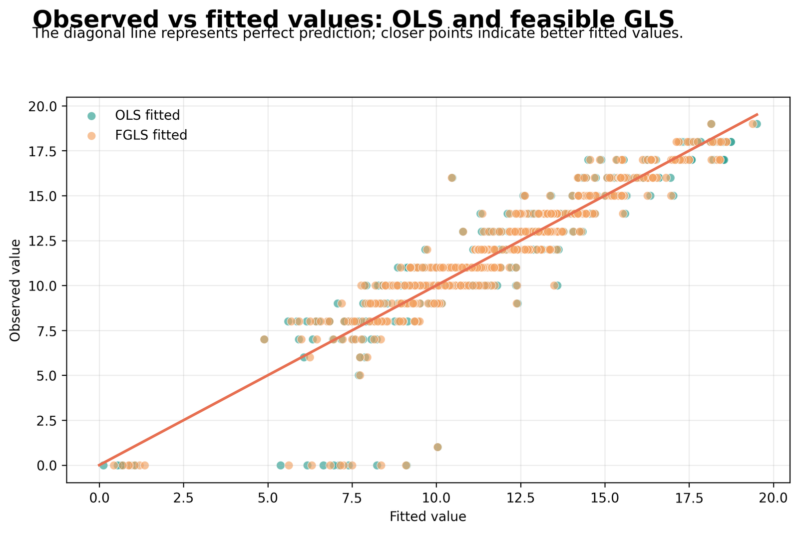
Both fitted series track the 45-degree line closely through the middle of the grade distribution. OLS has R² = 0.8524, RMSE = 1.2403 and MAE = 0.7791. FGLS has weighted R² = 0.8695, RMSE = 1.2423 and MAE = 0.7721.
The two point clouds overlap heavily because coefficient changes are modest. Several zero outcomes receive fitted values between approximately 5 and 10, producing large negative residuals. FGLS improves the weighted objective and MAE, but it does not eliminate these unusual cases.
Python Chart 3: OLS Residuals vs Fitted Values
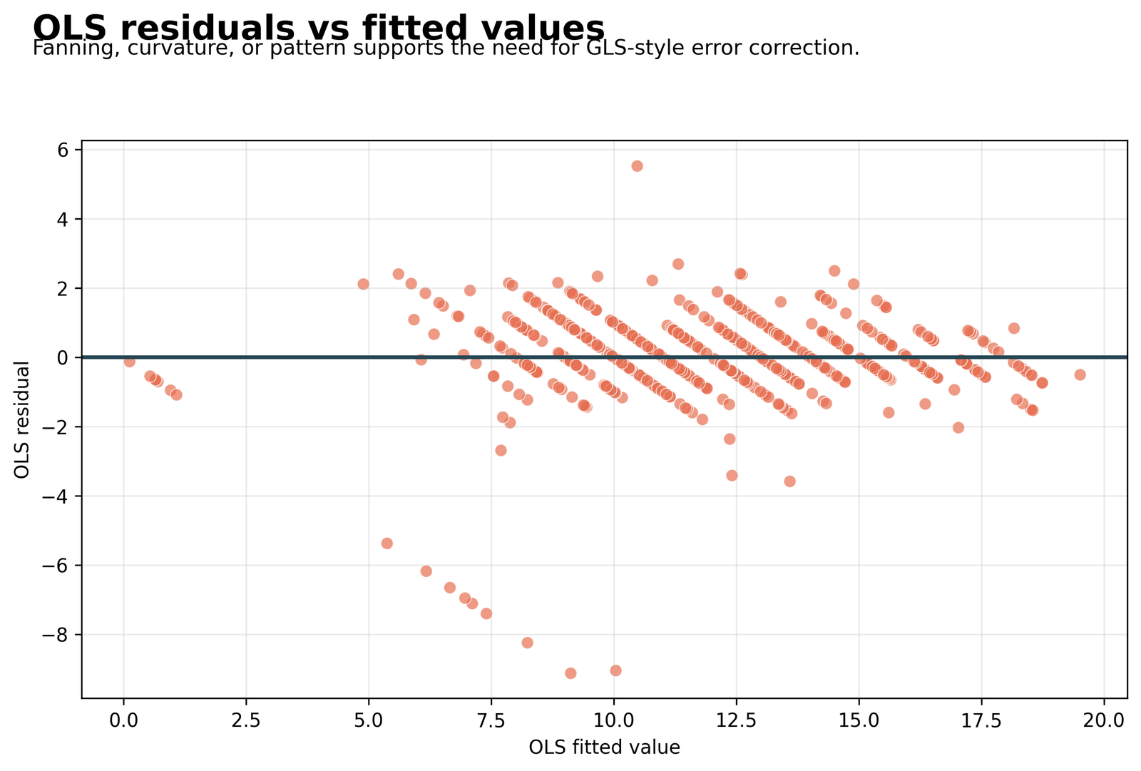
OLS residuals range visually from approximately -9.1 to 5.5. The main residual band is concentrated between about -2 and 2, but the distribution includes large negative points around fitted values 5–10. The diagonal stripes arise because observed G3 is integer valued while fitted values are continuous.
Formal tests confirm that the visible spread is not constant: Breusch–Pagan LM = 34.4086, p = 0.000157, and White LM = 106.8797, p = 0.000348. These values, rather than visual appearance alone, motivate the FGLS correction.
Python Chart 4: Feasible GLS Residuals vs Fitted Values
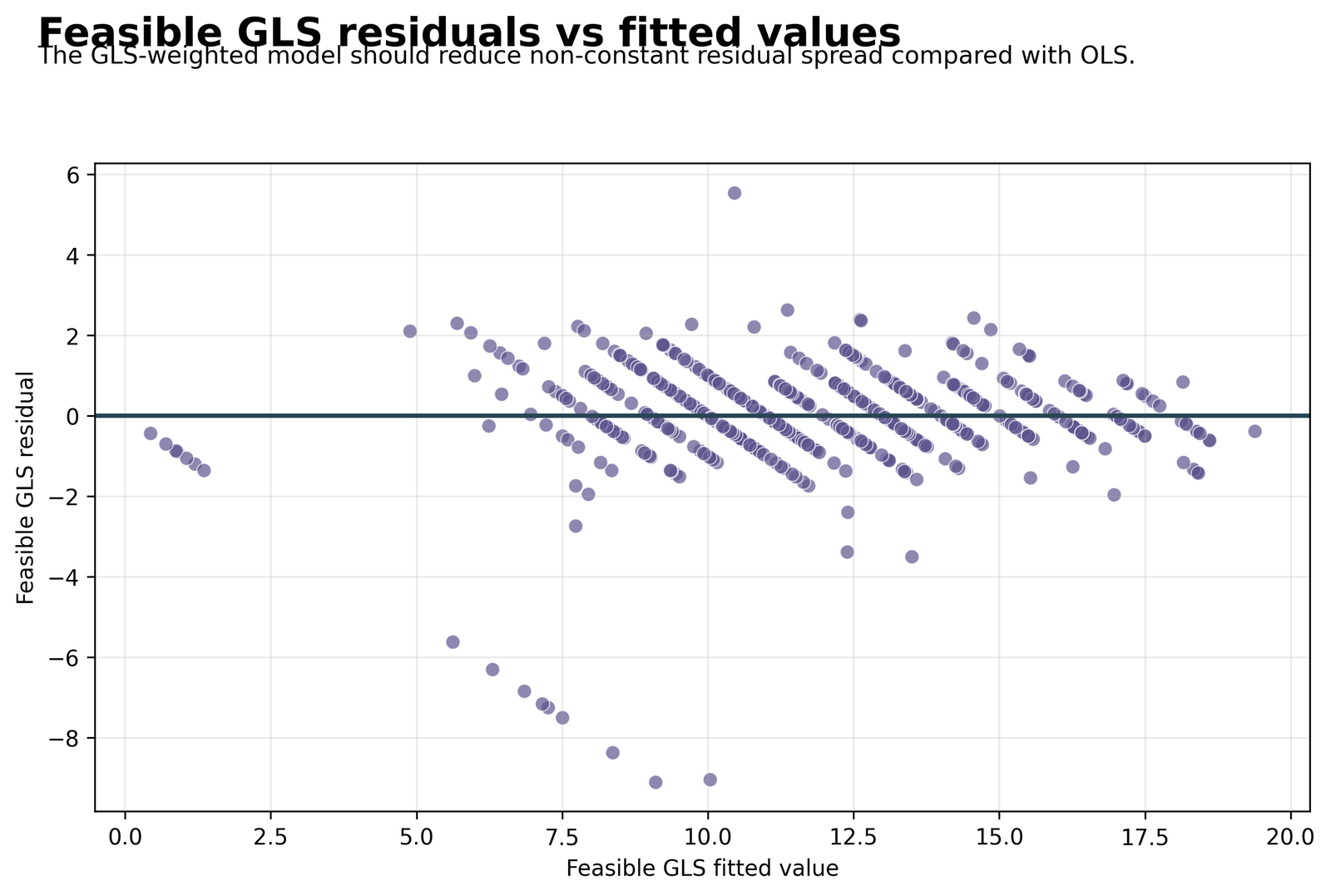
The FGLS residual plot retains a similar raw-residual range, approximately -9.1 to 5.6, because weighting does not guarantee smaller residuals for every observation. The central point band remains near zero and the same integer-outcome diagonal structure is visible.
FGLS MAE decreases from 0.7791 to 0.7721, but RMSE rises slightly from 1.2403 to 1.2423. The correct interpretation is not that every residual became smaller. The model redistributes influence according to estimated precision and improves the weighted likelihood and average absolute error.
Python Chart 5: OLS vs FGLS Absolute Residual Spread
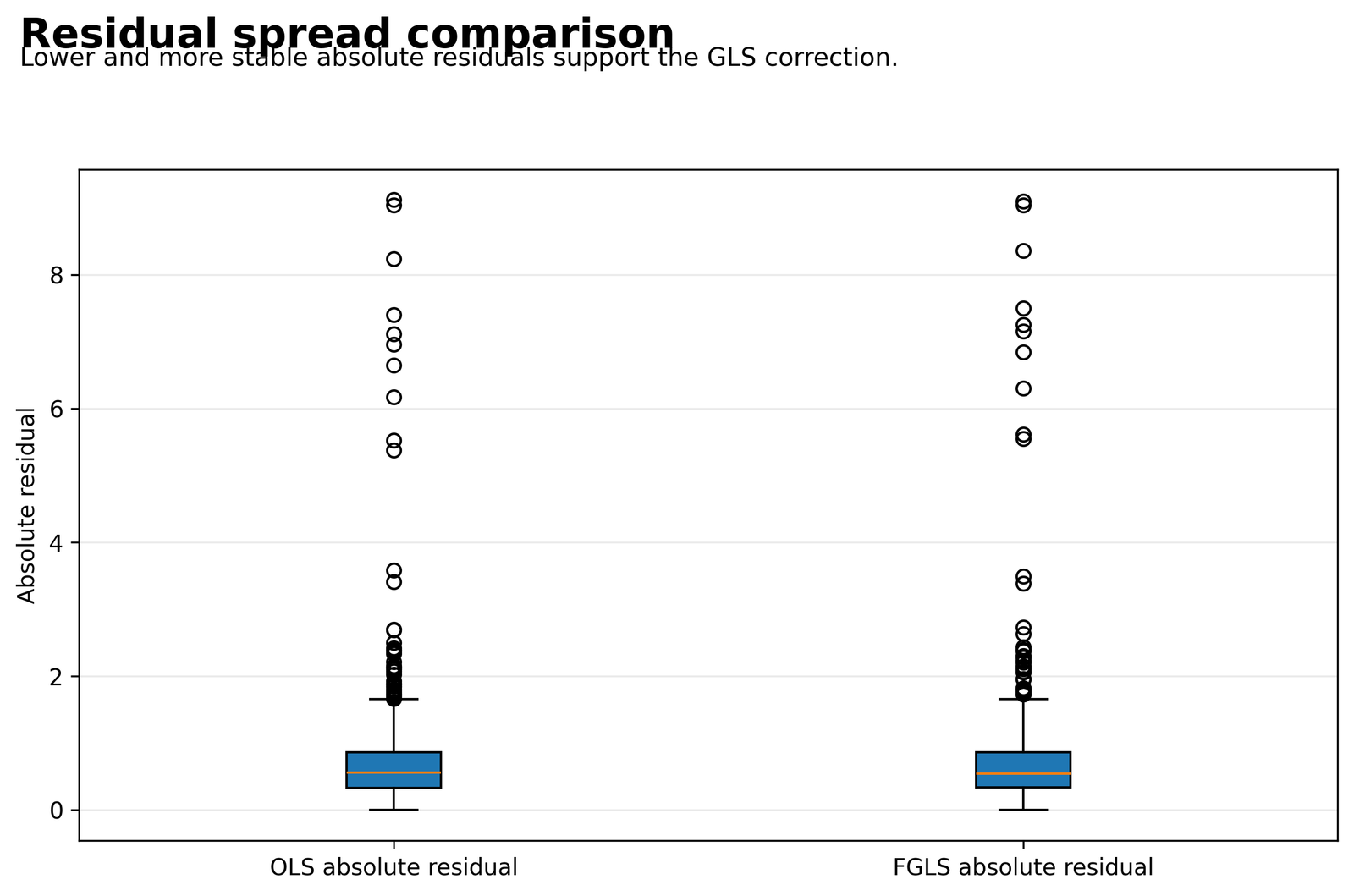
The two boxplots have very similar central ranges and extreme outliers reaching above 9. OLS MAE is 0.7791, while FGLS MAE is 0.7721, an improvement of about 0.0070. The boxplot median appears slightly lower for FGLS, but the difference is small.
The chart is a useful warning against exaggerated claims. GLS is strongly justified by the variance diagnostics, yet the unweighted absolute-residual distribution changes only modestly. Efficiency correction and dramatic point-prediction improvement are not the same thing.
Python Chart 6: OLS vs Feasible GLS Coefficient Comparison
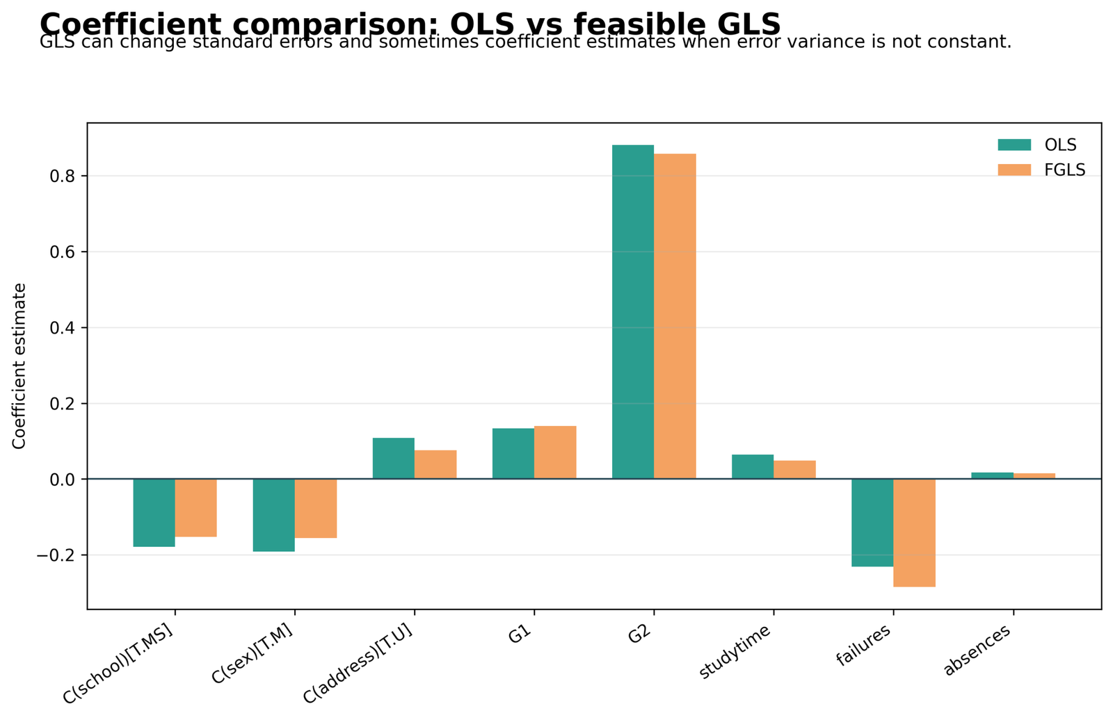
OLS plotted coefficients are school_MS = -0.1788, sex_M = -0.1917, address_U = 0.1082, G1 = 0.1337, G2 = 0.8814, studytime = 0.0641, failures = -0.2315 and absences = 0.0177. The FGLS bars remain close but shift approximately to -0.15, -0.16, 0.08, 0.14, 0.86, 0.05, -0.29 and 0.01.
G2 remains the dominant effect under both estimators. The largest visible change occurs for failures, which becomes more negative under FGLS. Exact FGLS coefficients should be copied from the output CSV because the PDF coefficient table is truncated.
Python Chart 7: Feasible GLS Weight Distribution
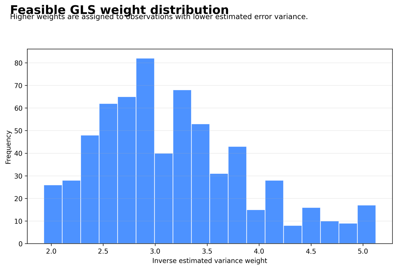
Weights span approximately 1.9 to 5.1. The highest-frequency bin is around 2.8–3.0 with slightly more than 80 observations. Other dense regions occur around 2.5–2.8 and 3.1–3.5. Relatively few records receive weights above 4.5.
The moderate range indicates that the variance model changes influence without creating extremely dominant observations. Higher weights correspond to lower predicted error variance; lower weights correspond to noisier observations.
Python Chart 8: OLS Diagnostic p-Values
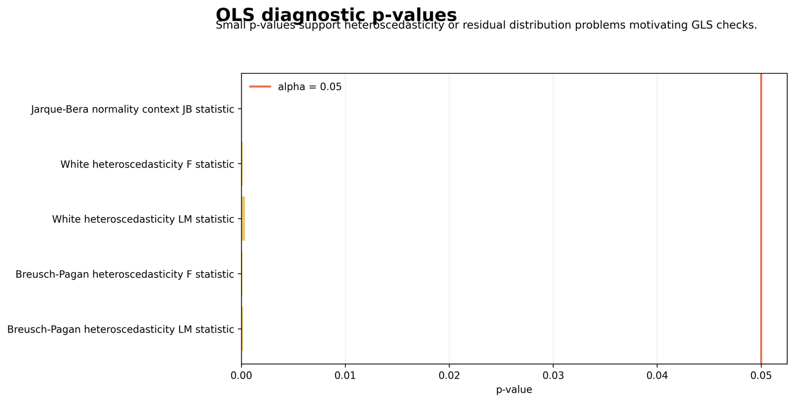
Every displayed p-value is far left of the .05 reference line. Python reports Breusch–Pagan LM p = 0.000157, Breusch–Pagan F p near 0.0001, White LM p = 0.000348, White F p near 0.0001 and Jarque–Bera p < 0.0001.
The heteroscedasticity tests support GLS. The Jarque–Bera result supports residual-distribution caution but does not determine the choice between OLS and GLS. Durbin–Watson is excluded because it is a statistic rather than a p-value.
Python Chart 9: Observed and Fitted Means by G1
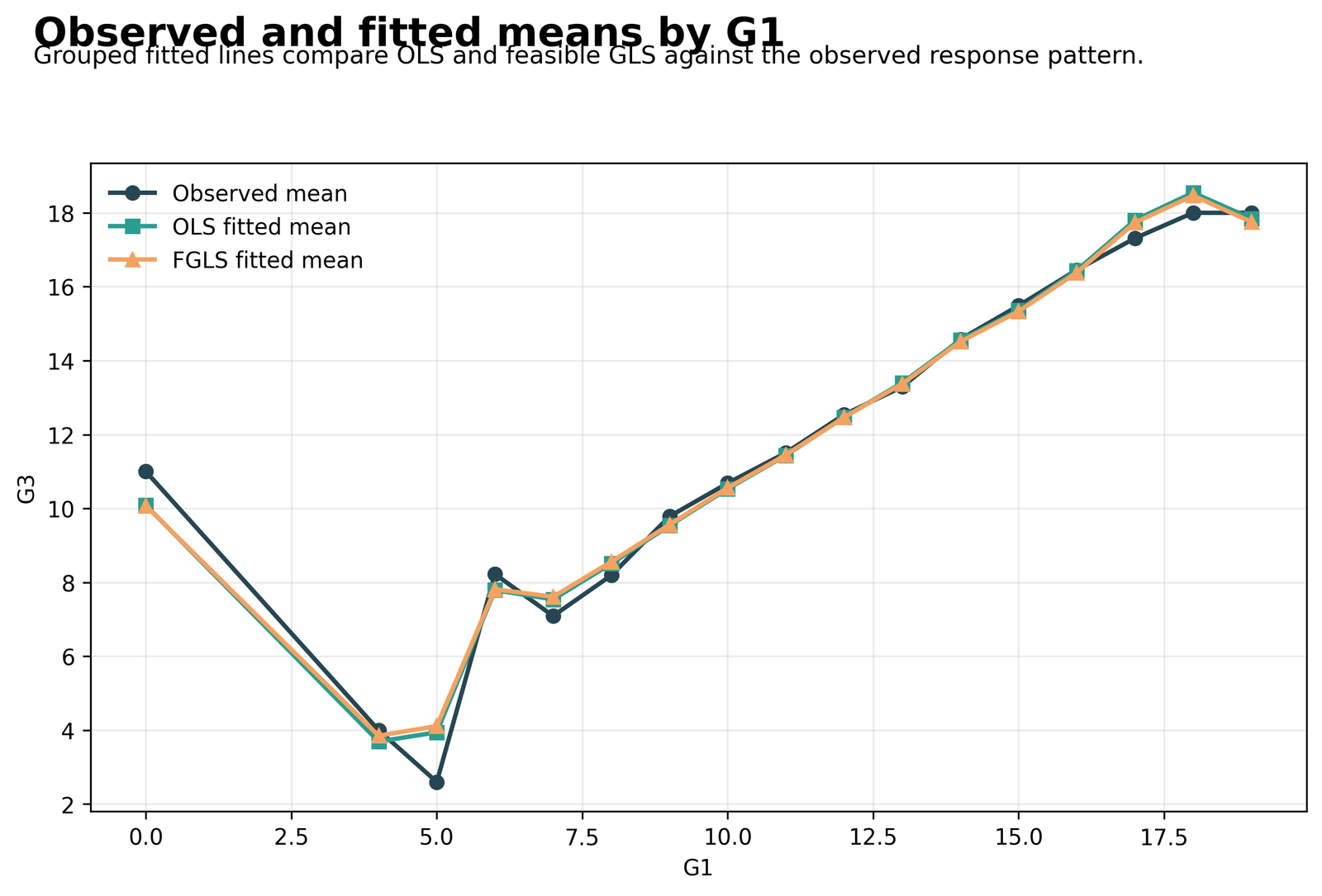
At G1 = 0, the observed mean is approximately 11.0, while OLS and FGLS means are near 10.1. At G1 = 5, the observed mean is approximately 2.6, whereas both fitted means are near 4.0. From G1 = 8 through 17, the three lines generally track closely.
At G1 = 18, the fitted means rise to about 18.5, compared with an observed mean near 18.0. At G1 = 19, the observed mean is about 18.0 and fitted means are about 17.7–17.8. The chart shows excellent central calibration with larger discrepancies at sparse extreme G1 levels.
R Charts, Tables and Independent Validation
The R report independently reproduces the 649-row formula, heteroscedasticity decision, model comparison and nine chart topics. The supplied list repeats the same chart URLs, so the R section uses those confirmed assets while interpreting the R-specific numerical results.
Open the complete Generalized Least Squares Regression R report PDF
R Chart 1: Outcome Distribution Validation
R uses the same outcome mean 11.9060, median 12, SD 3.2307 and range 0–19. This confirms that OLS and FGLS differences are estimator differences rather than changes in the analyzed sample.
R Chart 2: Observed vs Fitted Validation
R reports OLS RMSE = 1.240328 and MAE = 0.7790877. FGLS reports RMSE = 1.242313 and MAE = 0.7721485. The same conclusion holds: average absolute error improves slightly, while RMSE changes minimally in the opposite direction.
R Chart 3: OLS Residual Diagnostic Validation
R’s Breusch–Pagan LM statistic is 19.0968 with p = 1.24 × 10⁻⁵. The White statistic is 20.0366 with p = 4.46 × 10⁻⁵. Both validate the nonconstant variance decision despite differing from Python’s auxiliary-test statistics.
R Chart 4: FGLS Residual Diagnostic Validation
The weighted fit modifies the coefficient solution and influence structure, but raw residual outliers remain. Post-FGLS residual checks should evaluate whether the variance relationship is reduced in transformed or standardized residuals, not only whether every raw residual shrinks.
R Chart 5: Residual Spread Validation
R MAE decreases by approximately 0.00694. The boxplots remain similar because the strongest correction is to observation influence and likelihood, not a universal compression of raw residual magnitudes.
R Chart 6: Coefficient Comparison Validation
R reproduces exact OLS coefficients G1 = 0.133732, G2 = 0.881441 and failures = -0.231465. The FGLS comparison preserves the dominant G2 effect and negative failures direction.
R Chart 7: Weight Distribution Validation
The distribution concentrates between approximately 2 and 4, with a thinner upper tail to about 5.1. This indicates meaningful but not extreme reweighting.
R Chart 8: Diagnostic p-Value Validation
R’s heteroscedasticity p-values are even smaller than Python’s: 0.0000124 and 0.0000446. Both are far below .05. Jarque–Bera is effectively zero, confirming nonnormal residual tails.
R Chart 9: Observed and Fitted Means by G1 Validation
The observed and fitted mean lines nearly overlap for most G1 values, with the largest discrepancy near G1 = 5. R therefore confirms strong central fit and sparse-level instability at the extremes.
R validation conclusion: R reproduces the same model hierarchy and practical conclusion as Python. FGLS is justified by heteroscedasticity and improves the weighted fit and MAE, while the basic academic coefficient pattern remains stable.
SPSS Output Status and Corrected GLS Workflow
Open the currently supplied SPSS PDF
Current file is invalid: the one-page PDF contains only an SPSS warning that EMBEDBOOKMARKS is not a recognized subcommand and that command execution stopped. It contains no regression model summary, ANOVA table, coefficient table, saved residuals or weight diagnostics.
Required SPSS Export Correction
OUTPUT EXPORT
  /CONTENTS EXPORT=ALL LAYERS=PRINTSETTING MODELVIEWS=PRINTSETTING
  /PDF DOCUMENTFILE=
'D:\DATA ANALYSIS\H Regression Tests and Models\Generalized Least Squares Regression\SPSS_Output\pdf\generalized_least_squares_regression_spss_report.pdf'.
Do not use EMBEDBOOKMARKS or EMBEDFONTS as separate OUTPUT EXPORT subcommands. Regenerate the Viewer output and PDF after removing them.
Practical SPSS FGLS Procedure
SPSS does not provide the same one-command heteroscedastic FGLS workflow as the Python/R scripts. A compatible approach is:
- Fit baseline REGRESSION and save predicted values and residuals.
- Compute squared residuals and log squared residuals with a small constant.
- Regress log residual squared on absolute fitted value or selected variance predictors.
- Save predicted log variance.
- Compute estimated variance as EXP(predicted log variance).
- Compute inverse variance weight.
- Use WLS or weighted REGRESSION with the estimated weight.
- Save a valid SAV, SPV and PDF.
| Expected SPSS Output | Required Content | Current Status |
|---|---|---|
| Case processing | N = 649 complete observations. | Missing |
| OLS model summary | R², adjusted R², standard error. | Missing |
| OLS coefficients | B, SE, t, Sig., 95% CI. | Missing |
| Variance model | Predicted log variance and weights. | Missing |
| Weighted regression | FGLS coefficient table and model summary. | Missing |
| Diagnostics | Residual charts, BP/White equivalent context and DW. | Missing |
| PDF export | Compatibility-safe OUTPUT EXPORT. | Failed due obsolete subcommand |
Excel Worked Generalized Least Squares Results
The Excel workbook is a separate 10-row formula demonstration. It does not reproduce the 649-row model coefficients. It explains how OLS residuals lead to estimated variances, inverse weights and FGLS fitted values.
Excel Demonstration Summary
| Metric | Excel Value | Interpretation |
|---|---|---|
| Rows | 10 | Small teaching example. |
| OLS RMSE | 0.673795 | Root mean squared OLS residual. |
| FGLS RMSE | 0.459347 | Lower demonstration error after weighting. |
| Mean OLS absolute residual | 0.620000 | Average unweighted absolute OLS error. |
| Mean FGLS absolute residual | 0.410000 | Average absolute FGLS error. |
| Mean GLS weight | 0.305738 | Average inverse estimated variance. |
| Largest weight | 0.406570 | Most precise demonstration observation. |
| Smallest weight | 0.173774 | Least precise demonstration observation. |
Ten-Row Formula Demonstration
For row 1, observed Y = 10, OLS fitted = 10.4 and OLS residual = -0.4. The predicted log variance is 1.15, estimated variance is 3.1582, inverse weight is 0.3166, FGLS fitted = 10.2 and FGLS residual = -0.2.
Row 7 has the smallest weight, approximately 0.1738, because its estimated variance is 5.7546. Row 8 has the largest weight, approximately 0.4066, because its estimated variance is 2.4596. This directly demonstrates inverse-variance weighting.
Excel Formula Patterns
| Quantity | Formula Pattern | Purpose |
|---|---|---|
| OLS residual | =ObservedY-OLSFitted | Initial model error. |
| Residual squared | =OLSResidual^2 | Variance proxy. |
| Log residual squared | =LN(ResidualSquared+0.000001) | Variance-model outcome. |
| Estimated variance | =EXP(PredictedLogVariance) | Positive variance estimate. |
| GLS weight | =1/EstimatedVariance | Inverse estimated precision weight. |
| FGLS residual | =ObservedY-FGLSFitted | Weighted-model error. |
| RMSE | =SQRT(AVERAGE(ResidualSquaredRange)) | Root mean squared error. |
| MAE | =AVERAGE(AbsoluteResidualRange) | Mean absolute error. |
Do not mix workbook and full-data results: Excel RMSE 0.4593 describes the 10-row demonstration. The 649-row FGLS RMSE is 1.2423.
Python, R, SPSS and Excel GLS Workflows
| Software | Main Workflow | Outputs | Status |
|---|---|---|---|
| Python | statsmodels OLS, variance regression, WLS, GLS diagonal covariance and GLSAR. | Nine charts, CSV tables, TXT report and confirmed PDF. | Complete |
| R | lm baseline, variance model, weighted lm/FGLS and diagnostic tests. | Nine charts, CSV tables, TXT report and confirmed PDF. | Complete |
| SPSS | Baseline REGRESSION, saved residuals, variance model, computed weights and weighted regression. | SAV, SPV and PDF expected. | PDF export failed and must be regenerated |
| Excel | Ten-row residual, variance, weight and fitted-value formulas. | Worked explanatory workbook. | Complete teaching example |
Generalized Least Squares Regression Code
Python Code
import numpy as np
import pandas as pd
import statsmodels.api as sm
import statsmodels.formula.api as smf
from statsmodels.stats.diagnostic import het_breuschpagan, het_white
from statsmodels.stats.stattools import durbin_watson

df = pd.read_csv("dataset.csv")

formula = (
    "G3 ~ G1 + G2 + studytime + failures + absences + age + Medu"
    " + C(school) + C(sex) + C(address)"
)

work = df[
    ["G3", "G1", "G2", "studytime", "failures",
     "absences", "age", "Medu", "school", "sex", "address"]
].dropna().copy()

# OLS baseline
ols = smf.ols(formula, data=work).fit()
work["ols_fitted"] = ols.fittedvalues
work["ols_resid"] = ols.resid

# Heteroscedasticity tests
bp = het_breuschpagan(ols.resid, ols.model.exog)
white = het_white(ols.resid, ols.model.exog)
print("BP LM p:", bp[1])
print("White LM p:", white[1])
print("DW:", durbin_watson(ols.resid))

# Variance model
small = 1e-8
work["log_resid_sq"] = np.log(work["ols_resid"] ** 2 + small)
variance_model = smf.ols(
    "log_resid_sq ~ I(abs(ols_fitted))",
    data=work
).fit()

work["predicted_log_variance"] = variance_model.predict(work)
work["estimated_variance"] = np.exp(work["predicted_log_variance"])
work["gls_weight"] = 1.0 / work["estimated_variance"]

# Feasible GLS as WLS
fgls = smf.wls(
    formula,
    data=work,
    weights=work["gls_weight"]
).fit()

# Equivalent diagonal GLS
sigma = np.diag(work["estimated_variance"].to_numpy())
gls = sm.GLS(
    ols.model.endog,
    ols.model.exog,
    sigma=sigma
).fit()

print(fgls.summary())
print(gls.summary())
R Code
df <- read.csv("dataset.csv", stringsAsFactors = TRUE)

formula_gls <- G3 ~ G1 + G2 + studytime + failures +
  absences + age + Medu + school + sex + address

work <- na.omit(df[
  c("G3", "G1", "G2", "studytime", "failures",
    "absences", "age", "Medu", "school", "sex", "address")
])

ols <- lm(formula_gls, data = work)
work$ols_fitted <- fitted(ols)
work$ols_residual <- residuals(ols)

small <- 1e-8
work$log_resid_sq <- log(work$ols_residual^2 + small)

variance_model <- lm(
  log_resid_sq ~ abs(ols_fitted),
  data = work
)

work$predicted_log_variance <- predict(variance_model)
work$estimated_variance <- exp(work$predicted_log_variance)
work$gls_weight <- 1 / work$estimated_variance

fgls <- lm(
  formula_gls,
  data = work,
  weights = gls_weight
)

summary(ols)
summary(fgls)

library(lmtest)
library(sandwich)
bptest(ols)
dwtest(ols)
SPSS Compatibility-Safe Syntax Pattern
* Baseline OLS.
REGRESSION
  /DEPENDENT G3
  /METHOD=ENTER G1 G2 studytime failures absences age Medu
    school_MS sex_M address_U
  /STATISTICS COEFF OUTS R ANOVA CI(95) COLLIN TOL
  /SAVE PRED(ols_pred) RESID(ols_resid).

COMPUTE resid_sq = ols_resid**2.
COMPUTE log_resid_sq = LN(resid_sq + .000001).
COMPUTE abs_ols_pred = ABS(ols_pred).
EXECUTE.

* Variance model.
REGRESSION
  /DEPENDENT log_resid_sq
  /METHOD=ENTER abs_ols_pred
  /SAVE PRED(pred_log_variance).

COMPUTE estimated_variance = EXP(pred_log_variance).
COMPUTE gls_weight = 1 / estimated_variance.
EXECUTE.

WEIGHT BY gls_weight.

REGRESSION
  /DEPENDENT G3
  /METHOD=ENTER G1 G2 studytime failures absences age Medu
    school_MS sex_M address_U
  /STATISTICS COEFF OUTS R ANOVA CI(95) COLLIN TOL
  /SAVE PRED(fgls_pred) RESID(fgls_resid).

WEIGHT OFF.

OUTPUT SAVE OUTFILE=
'D:\DATA ANALYSIS\H Regression Tests and Models\Generalized Least Squares Regression\SPSS_Output\spv\generalized_least_squares_regression_spss_output.spv'.

OUTPUT EXPORT
  /CONTENTS EXPORT=ALL LAYERS=PRINTSETTING MODELVIEWS=PRINTSETTING
  /PDF DOCUMENTFILE=
'D:\DATA ANALYSIS\H Regression Tests and Models\Generalized Least Squares Regression\SPSS_Output\pdf\generalized_least_squares_regression_spss_report.pdf'.
Excel Formula Pattern
OLS residual:
=ObservedY-OLSFitted

Residual squared:
=OLSResidual^2

Log residual squared:
=LN(ResidualSquared+0.000001)

Estimated variance:
=EXP(PredictedLogVariance)

GLS inverse variance weight:
=1/EstimatedVariance

Weighted least squares objective:
=SUMPRODUCT(WeightRange,ResidualRange,ResidualRange)
Generalized Least Squares vs Heteroscedasticity-Robust Standard Errors
| Feature | GLS / FGLS | OLS with Robust SE |
|---|---|---|
| Coefficient estimates | Can change because observations are reweighted/transformed. | Remain equal to OLS coefficients. |
| Covariance model | Must be specified or estimated. | No explicit variance model required. |
| Efficiency | Can improve if Ω is well specified. | Consistent uncertainty but not necessarily efficient coefficients. |
| Misspecification risk | Incorrect weights can harm efficiency and inference. | More robust to unknown heteroscedasticity. |
| Prediction | Weighted fit may change predictions. | Predictions remain OLS predictions. |
| Recommended use | Strong, interpretable variance/dependence structure. | Heteroscedasticity is present but variance model is uncertain. |
A useful sensitivity analysis reports OLS with HC3 standard errors alongside FGLS. If substantive conclusions change dramatically, investigate whether a small set of weights or variance-model assumptions drives the difference.
Prediction, Fit and Model Selection in GLS
Weighted R² is calculated using the weighted residual objective and should not automatically be compared with unweighted OLS R² as though they were the same quantity. AIC and BIC also depend on likelihood conventions and weight scaling.
How to Interpret This Model Comparison
| Metric | OLS | FGLS | Conclusion |
|---|---|---|---|
| Weighted / reported R² | 0.8524 | 0.8695 | FGLS better under its weighted objective. |
| Adjusted R² | 0.8501 | 0.8674 | FGLS weighted fit remains higher after df adjustment. |
| MAE | 0.7791 | 0.7721 | Small FGLS improvement. |
| RMSE | 1.2403 | 1.2423 | Small OLS advantage on unweighted squared error. |
| AIC within Python | 2143.3400 | 2037.0053 | FGLS likelihood fit is much better under Python’s implementation. |
| Durbin–Watson | 1.8723 | 1.8716 | Weighting does not materially change weak serial dependence. |
For prediction, evaluate cross-validated unweighted error, weighted error and calibration across variance strata. In-sample weighted AIC improvement is not enough to establish superior out-of-sample prediction.
APA-Style Reporting for Generalized Least Squares Regression
Full Python Result
A feasible generalized least squares regression was fitted to predict G3 from G1, G2, studytime, failures, absences, age, maternal education, school, sex and address using 649 complete observations. OLS residual diagnostics indicated heteroscedasticity, Breusch–Pagan LM = 34.41, p < .001, and White LM = 106.88, p < .001. Durbin–Watson was 1.87, indicating little first-order residual dependence. Inverse estimated error-variance weights were derived from a log residual-variance model. The feasible GLS model reported R² = .870, adjusted R² = .867, MAE = .772 and RMSE = 1.242, compared with OLS R² = .852, adjusted R² = .850, MAE = .779 and RMSE = 1.240.
Coefficient Summary
The OLS and FGLS coefficient patterns were substantively similar. G2 remained the dominant positive predictor, OLS B = 0.881, 95% CI [0.814, 0.949], p < .001. G1 was positive, B = 0.134, 95% CI [0.061, 0.206], p < .001, and failures was negative, B = -0.231, 95% CI [-0.418, -0.045], p = .015. The FGLS coefficient-comparison chart showed modest weighting-related changes rather than sign reversals.
SPSS Qualification
The supplied SPSS PDF could not be interpreted because export stopped after an unrecognized EMBEDBOOKMARKS subcommand. SPSS results should be reported only after regenerating the output with the compatibility-safe OUTPUT EXPORT syntax.
Generalized Least Squares Reporting Checklist
| Reporting Item | Required Detail | Why It Matters |
|---|---|---|
| Outcome | Name, units and range. | Defines coefficient scale. |
| Predictors | Numeric variables, factors and reference levels. | Supports interpretation and replication. |
| OLS baseline | Coefficients, fit and residual diagnostics. | Shows why GLS was considered. |
| Covariance problem | Heteroscedasticity, autocorrelation or clustering. | Defines the correction target. |
| Variance/correlation model | Exact equation or covariance structure. | FGLS depends on this specification. |
| Weight construction | Inverse known or estimated variance. | Explains differential influence. |
| Weight range | Minimum, maximum and quantiles. | Identifies influential precision weights. |
| GLS coefficient table | B, SE, statistic, p and 95% CI. | Primary inferential result. |
| Model comparison | R² type, AIC/BIC, MAE and RMSE. | Prevents metric cherry-picking. |
| Post-fit diagnostics | Weighted/standardized residual checks. | Evaluates covariance correction quality. |
| Sensitivity analysis | OLS robust SE and alternative variance models. | Tests dependence on FGLS assumptions. |
| Software details | Package, tie/likelihood convention and weight scaling. | Explains implementation differences. |
Common Generalized Least Squares Mistakes
| Mistake | Why It Is Wrong | Better Practice |
|---|---|---|
| Using GLS only because OLS residuals are nonnormal | GLS targets covariance, not distribution shape alone. | Identify heteroscedasticity or dependence explicitly. |
| Treating arbitrary case weights as inverse variances | The estimator no longer has the intended precision interpretation. | Document where every weight comes from. |
| Claiming FGLS improves every prediction metric | Here MAE improves but RMSE slightly worsens. | Report all relevant metrics. |
| Comparing AIC across Python and R directly | Likelihood constants and weight conventions differ. | Compare candidate models within the same software. |
| Ignoring weight extremes | A few high weights can dominate coefficients. | Inspect distribution and sensitivity to trimming. |
| Using FGLS without post-fit diagnostics | The estimated variance model may remain inadequate. | Review weighted and standardized residuals. |
| Assuming GLS fixes endogeneity | It changes error covariance, not predictor exogeneity. | Use design or instrumental-variable methods. |
| Reporting the current SPSS PDF as output | It contains only an export error. | Regenerate SAV/SPV/PDF with safe syntax. |
| Using the GEE PDF in the GLS post | GEE is a different correlated-data estimator. | Keep Generalized Estimating Equations in its own article. |
Generalized Least Squares Troubleshooting Guide
Weights Are Infinite or Missing
Predicted variance may be zero, negative before exponentiation, missing or numerically extreme. Use a log-variance model, verify finite fitted values and apply reasonable numerical bounds only with documented justification.
FGLS Coefficients Change Dramatically
Inspect whether a small number of observations receive very large weights. Compare with OLS HC3 results and refit after checking data errors. Dramatic changes may indicate variance-model misspecification.
FGLS R Squared Is Higher but RMSE Is Worse
This is possible because weighted R² optimizes a different objective than unweighted RMSE. In this analysis, FGLS adjusted R² rises to .8674 while RMSE changes from 1.2403 to 1.2423.
Python and R AIC Values Differ by a Constant
Different implementations include different likelihood constants or weight normalizations. Compare differences between OLS and FGLS inside Python or inside R, not raw values across languages.
Breusch–Pagan and White Statistics Differ Across Software
The auxiliary regressions and degrees of freedom may differ. Focus on whether the same null decision is reached. Here every implementation strongly rejects constant variance.
Durbin–Watson Is Near 2 but GLSAR Is Included
GLSAR is a comparison model. With ρ = 0.0661 and DW = 1.8723, autocorrelation is weak; the main correction remains heteroscedastic FGLS.
SPSS PDF Contains Only EMBEDBOOKMARKS Error
Remove the unsupported subcommand, rerun the entire syntax, save the Viewer file and export with the safe PDF block. Do not merely rename the failed one-page PDF.
FGLS Residual Plot Still Has Outliers
GLS does not guarantee elimination of unusual outcomes. Check studentized residuals, Cook’s distance, Mahalanobis distance and outlier detection.
Variance Model Produces No Improvement
The chosen variance predictor may not describe heteroscedasticity. Consider multiple variance predictors, group-specific variances, smooth functions or robust OLS instead of forcing FGLS.
Downloads and Resources
R GLS Report PDFConfirmed 13-page R report with model validation and nine charts.
Current SPSS PDF — Regeneration RequiredContains only the EMBEDBOOKMARKS export error; not valid analysis output.
Worked Excel FileExpected hosted filename for the 10-row formula and interpretation workbook.
FAQs About Generalized Least Squares Regression
What is generalized least squares regression?
GLS is linear regression that estimates coefficients while accounting for unequal error variances or correlations through an error covariance matrix.
What is feasible generalized least squares?
FGLS estimates the unknown error covariance from preliminary residuals and then fits GLS using the estimated covariance.
Why was GLS used in this example?
Breusch–Pagan and White tests strongly rejected constant OLS error variance, while Durbin–Watson showed only weak serial dependence.
What variables were used?
G3 was predicted from G1, G2, studytime, failures, absences, age, Medu, school, sex and address.
What was the FGLS adjusted R squared?
The Python report gives adjusted R² = 0.8674, compared with 0.8501 for OLS.
Did FGLS improve prediction?
MAE improved slightly from 0.7791 to 0.7721, while RMSE changed slightly from 1.2403 to 1.2423. Improvement depends on the metric and weighting objective.
What is the GLS weight?
The workflow uses the inverse of estimated observation-specific error variance. Higher weights indicate greater estimated precision.
Is WLS the same as GLS?
WLS is a special case of GLS with a diagonal covariance matrix. General GLS can also model correlations between errors.
Is GLS better than robust standard errors?
GLS can be more efficient when the covariance model is correct. Robust OLS requires fewer covariance assumptions and keeps OLS coefficients.
Why do Python and R AIC values differ?
The packages use different likelihood constants or weight scaling. Model comparisons should be made within each software.
Was autocorrelation a major problem?
No. Durbin–Watson was 1.8723 and the GLSAR rho estimate was only 0.0661.
Can GLS be done in SPSS?
Yes through a saved-residual variance model and weighted regression, but the supplied PDF failed during export and must be regenerated.
What is wrong with the supplied SPSS PDF?
It contains only an error saying EMBEDBOOKMARKS is not recognized. No regression results were exported.
Can GLS be calculated in Excel?
Excel can demonstrate residual variance, inverse weights and weighted fitted values. Python or R is preferable for complete coefficient estimation and diagnostics.
Does GLS fix endogeneity?
No. GLS corrects the error covariance structure. It does not make endogenous predictors exogenous.
Final Generalized Least Squares Regression Conclusion
The 649-row analysis provides strong evidence that OLS errors are heteroscedastic. Feasible GLS uses inverse estimated error-variance weights and increases the reported weighted adjusted R² from 0.8501 to 0.8674. It lowers MAE from 0.7791 to 0.7721 and substantially improves within-software likelihood criteria, while unweighted RMSE remains nearly unchanged.
G2 remains the dominant academic predictor, G1 remains positive, and failures remains negative. The correction changes coefficient magnitude and influence modestly rather than reversing the substantive model.
The correct final report should state the variance model, explain the weight construction, distinguish weighted from unweighted fit measures, provide sensitivity analysis against robust OLS and regenerate the SPSS output with compatibility-safe PDF syntax before publishing SPSS-specific numerical conclusions.

