
Gaussian, Binomial and Poisson Regression in One Unified Framework
Generalized Linear Model: Formula, Interpretation, SPSS, Python, R and Excel Guide
Generalized Linear Models connect an outcome distribution to a linear predictor through a link function. This complete Salar Cafe guide uses three fully named outcomes: continuous final grade G3, binary pass status glm_pass, and absence count glm_count. It reports exact model-fit values, coefficients, diagnostics, seven Python charts, two distinct R chart exports, worked Excel calculations, SPSS procedures, reproducible code and APA reporting.
Quick Answer: Generalized Linear Model Results
The analysis fits three separate GLMs to the same 649-student dataset. The Gaussian identity-link model predicts G3. The binomial logit-link model predicts glm_pass = 1 when G3 is at least 10. The Poisson log-link model predicts glm_count, created by rounding absences and clipping negative values at zero.
All three models use G1, G2, studytime, failures, age, Medu, Fedu, school, sex, and address. The Gaussian model has deviance 1002.1000 and AIC 2145.7210. The binomial model has deviance 176.1896 and AIC 198.1896. The Poisson model has deviance 3067.1642, AIC 4462.2974, and a Pearson dispersion ratio of approximately 4.9549.
Gaussian conclusion: G1, G2 and failures are statistically significant. G2 is the dominant predictor, B = 0.8804, SE = 0.0343, p < .001, 95% CI [0.8131, 0.9477].
Binomial conclusion: the model provides probabilities and odds ratios, but calibration must be interpreted together with discrimination, classification and the large Pearson statistic.
Poisson conclusion: severe overdispersion means the simple Poisson variance is not adequate. Negative-binomial, quasi-Poisson, hurdle or zero-inflated alternatives should be evaluated according to the scientific count process.
Table of Contents
- What Is a Generalized Linear Model?
- Why Use a Generalized Linear Model?
- Generalized Linear Model Formula
- How to Interpret GLM Coefficients
- Link Functions and Response Scales
- IRLS, Deviance and Robust Inference
- GLM vs Linear, GAM, GEE and Mixed Models
- Gaussian, Binomial and Poisson Families
- GLM Assumptions and Requirements
- Variables Used and Data Dictionary
- Python GLM Design
- Python Model-Fit and Coefficient Results
- Python Chart-by-Chart Interpretation
- Binomial Calibration and Poisson Overdispersion
- R GLM Design and Reproduction Workflow
- R Verification Results
- R-Specific Chart Exports
- How to Choose a GLM Family and Model
- Dispersion, Exposure and Count-Model Issues
- GLM Residuals, Influence and Diagnostics
- Worked Excel File
- SPSS Generalized Linear Model Workflow
- Python, R and SPSS Code
- APA-Style Reporting
- Common GLM Mistakes
- Generalized Linear Model Downloads
- Related Salar Cafe Statistical Guides
- FAQs About Generalized Linear Models
What Is a Generalized Linear Model?
A Generalized Linear Model, usually abbreviated as GLM, is a flexible regression framework that allows the expected value of an outcome to be modeled as a function of one or more predictor variables even when the outcome is not normally distributed. It extends ordinary linear regression by separating the analysis into three connected parts: the probability distribution of the outcome, the linear predictor formed from the explanatory variables, and a link function that connects the expected outcome to that linear predictor.
Ordinary linear regression assumes that the outcome is continuous, that its conditional mean is a direct linear combination of the predictors, and that the residual variance is constant. These assumptions are suitable for many measurements, such as height, weight, income after an appropriate transformation, or the final grade G3 used in this post. They are not suitable for every statistical outcome. A pass/fail response contains only two possible values, and an absence count cannot be negative. Generalized Linear Models preserve the familiar regression structure while adapting the outcome distribution and prediction scale to the type of data being analyzed.
In this expression, Yi is the outcome for observation i, E[Yi | Xi] is its conditional expected value, g() is the link function, ηi is the linear predictor, β0 is the intercept, and the remaining β coefficients represent adjusted predictor effects. The predictors may be continuous, ordinal, binary, categorical, transformed, or combined through interactions.
Why the Word “Generalized” Is Used
The model is called generalized because it generalizes the structure of ordinary linear regression to several outcome distributions. The Gaussian identity-link model reproduces conventional multiple linear regression. A binomial logit-link model produces logistic regression. A Poisson log-link model produces Poisson regression. These models look different in practical use, but they share the same mathematical framework.
The framework is not “general” in the sense that every possible statistical model is a GLM. Standard GLMs usually use outcome distributions from the exponential family and assume that observations are independent after conditioning on the predictors. Models with random effects, smooth nonlinear functions, zero-generating processes, serial dependence, survival times, latent variables, or complex mixtures may require extensions or different methods.
The Three Connected Parts of a GLM
| GLM Component | Statistical Meaning | Worked Example in This Post |
|---|---|---|
| Random component | Specifies the probability distribution and variance pattern of the outcome. | Gaussian for G3, binomial for glm_pass, and Poisson for glm_count. |
| Systematic component | Combines the predictors in the linear predictor η = Xβ. | G1, G2, studytime, failures, age, Medu, Fedu, school, sex, and address. |
| Link function | Transforms the expected outcome so it can be represented by the unrestricted linear predictor. | Identity for expected G3, logit for pass probability, and log for expected absences. |
1. The Random Component
The random component identifies the probability distribution used for the outcome and determines how the conditional variance is expected to behave. In a Gaussian GLM, the conditional variance is estimated as a separate scale parameter and is treated as approximately constant. In a binomial GLM, the variance depends on the event probability through p(1 − p). In a Poisson GLM, the theoretical variance equals the conditional mean.
This distributional choice is not a cosmetic software setting. It determines the likelihood, standard errors, deviance, residual definitions, confidence intervals, and valid coefficient interpretation. A continuous grade should not normally be forced into a Poisson model, and an absence count should not be analyzed with ordinary linear regression without first considering its nonnegative, discrete, and potentially overdispersed nature.
2. The Systematic Component
The systematic component is the familiar regression equation constructed from the predictors. It is called the linear predictor because coefficients and model terms enter additively on the link scale. The word linear refers to linearity in the coefficients, not necessarily to a simple straight-line relationship in the raw outcome.
For example, the Gaussian model in this post predicts G3 from G1, G2, studytime, failures, age, parental education, school, sex, and address. The binomial and Poisson models use the same systematic component but apply it to different transformed expected outcomes. Categorical variables enter through indicator contrasts, and interaction or polynomial terms may be added when theoretically justified.
The systematic component can therefore contain terms such as G2, G2², school × G2, or a transformed absence measure. However, a standard GLM still assumes that the transformed expected outcome is an additive linear combination of the specified terms. If the functional shape is unknown and smoothly nonlinear, a Generalized Additive Model may be more appropriate.
3. The Link Function
The link function connects the expected outcome to the linear predictor. It allows the unrestricted value of η, which can range from negative infinity to positive infinity, to produce predictions that respect the outcome’s valid range.
| Outcome | Link | Why the Link Is Useful | Inverse-Link Prediction |
|---|---|---|---|
| Continuous G3 | Identity | No transformation is needed because expected grade is modeled directly. | μ = η |
| Binary glm_pass | Logit | Maps every real-valued η to a probability between 0 and 1. | p = 1 / (1 + e−η) |
| Count glm_count | Log | Maps every real-valued η to a positive expected count. | μ = eη |
The link function also determines the coefficient scale. Under the identity link, a coefficient is an adjusted mean difference in outcome units. Under the logit link, a coefficient is an adjusted change in log odds, and its exponential is an odds ratio. Under the log link, a coefficient is an adjusted change in log rate, and its exponential is a rate ratio.
How the Same Predictors Produce Different Statistical Questions
The three models in this post use the same predictor set but do not answer the same question. The Gaussian model asks how G1, G2, studytime, failures, age, parental education, school, sex, and address relate to expected final-grade points. The binomial model asks how those predictors relate to the probability and odds of achieving G3 ≥ 10. The Poisson model asks how they relate to the expected number of absences.
Because the outcomes differ, their likelihoods, residuals, coefficients, confidence intervals, and AIC values are not directly interchangeable. A predictor can be strongly related to G3 while having little association with absence count. The same numerical coefficient would also have different meanings under identity, logit, and log links.
GLM as a Family of Regression Models
| Common Model | GLM Family | Link Function | Typical Outcome |
|---|---|---|---|
| Ordinary multiple linear regression | Gaussian | Identity | Continuous measurement. |
| Binary logistic regression | Binomial | Logit | Event versus non-event. |
| Probit regression | Binomial | Probit | Binary probability modeled through a normal cumulative function. |
| Poisson regression | Poisson | Log | Nonnegative event count. |
| Gamma regression | Gamma | Log or inverse | Positive, right-skewed continuous outcome. |
What a GLM Estimates
A GLM estimates a conditional mean rather than reproducing every individual outcome perfectly. The Gaussian model estimates the expected G3 for a given predictor profile. The binomial model estimates the probability of passing. The Poisson model estimates the expected absence count. Individual observations can differ substantially from these expected values because of unmeasured factors, random variation, unusual circumstances, and model misspecification.
Maximum-likelihood estimation identifies the coefficient values that make the observed outcomes most plausible under the selected family and link. Software commonly uses Iteratively Reweighted Least Squares to obtain these estimates. Model adequacy is then assessed using deviance, Pearson chi-square, residuals, influence measures, calibration, dispersion, information criteria, and validation performance.
What a GLM Does Not Automatically Solve
Choosing a GLM does not automatically correct nonlinear predictor effects, multicollinearity, omitted variables, influential observations, clustering, repeated measurements, missing-data bias, overdispersion, zero inflation, or causal confounding. These issues require separate diagnosis and, where necessary, a different model or an extension of the GLM framework.
| Problem | Why Standard GLM May Be Insufficient | Possible Alternative or Extension |
|---|---|---|
| Smooth nonlinear effects | One constant coefficient may not describe the relationship. | Generalized Additive Model. |
| Repeated or clustered observations | Independence assumption is violated. | Generalized Estimating Equations or generalized mixed model. |
| Poisson overdispersion | Conditional variance is much larger than the mean. | Negative-binomial or quasi-Poisson regression. |
| Excess structural zeros | One count-generating process may not explain all zeros. | Hurdle or zero-inflated model. |
| Individual random effects | Population mean alone does not model subject-specific variation. | Mixed-effects model. |
| Time-to-event outcome | Censoring and hazard structure are not represented. | Cox regression or accelerated failure-time model. |
Why GLMs Are Useful in Applied Research
GLMs allow researchers to use one coherent modeling language across different outcome types. Predictors, interactions, categorical contrasts, confidence intervals, hypothesis tests, predicted values, and model diagnostics can all be organized within the same framework. This consistency makes it easier to move from continuous regression to binary or count regression without treating each method as an unrelated procedure.
The framework also provides interpretable transformed effects. Odds ratios summarize multiplicative changes in odds, and rate ratios summarize multiplicative changes in expected counts. Predicted probabilities and expected counts can then be calculated for meaningful covariate patterns, making the model useful for explanation, classification, forecasting, and decision support.
Worked Meaning in the Student Dataset
For the Gaussian model, the statistically significant G2 coefficient of 0.8804 means that one additional G2 point is associated with approximately 0.880 additional expected G3 points after controlling the other predictors. The significant failures coefficient of −0.2253 represents a negative adjusted difference in expected G3 points.
For the binomial model, coefficients operate on the log-odds scale and must be exponentiated for odds-ratio interpretation. For the Poisson model, coefficients operate on the log expected-count scale and their exponentials are rate ratios. The Poisson model’s dispersion ratio of approximately 4.9549 demonstrates that selecting the correct outcome family must be followed by checking whether its variance assumption is actually supported.
Core interpretation: a Generalized Linear Model is not one single regression test. It is a family of regression models that combines an outcome distribution, a linear predictor, and a link function so that continuous means, event probabilities, and expected counts can be analyzed with statistically appropriate prediction scales.
Important distinction: the term GLM can also be used in some software to mean the “General Linear Model,” covering ANOVA, ANCOVA, and ordinary linear regression. In this article, GLM means Generalized Linear Model, which includes Gaussian, binomial, Poisson, Gamma, and related outcome families.
Why Use a Generalized Linear Model?
Ordinary linear regression is a special case of the generalized linear-model framework. It uses a Gaussian response distribution, identity link and constant conditional variance. GLM extends this structure to binary probabilities, counts and other supported outcomes without forcing every response into an ordinary least-squares model.
| Feature | Ordinary Linear Regression | Generalized Linear Model |
|---|---|---|
| Outcome | Normally treated as continuous. | Continuous, binary, count and other exponential-family outcomes. |
| Mean scale | Outcome mean is directly linear in predictors. | A link-transformed mean is linear in predictors. |
| Variance | Usually constant conditional variance. | Variance depends on the selected family and mean. |
| Coefficient scale | Outcome-unit mean difference. | Mean difference, log odds, log rate or another link-scale effect. |
| Estimation | Ordinary least squares. | Maximum likelihood, commonly through IRLS. |
The Gaussian model in this post is therefore both a GLM and a standard multiple linear regression. The binomial and Poisson models require GLM because probabilities must remain between zero and one and expected counts must remain nonnegative.
Research Questions Answered by the Three Models
| Question | Outcome | Model |
|---|---|---|
| How do predictors change expected final grade? | G3 | Gaussian identity GLM. |
| How do predictors change pass probability and odds? | glm_pass | Binomial logit GLM. |
| How do predictors change expected absence rate? | glm_count | Poisson log GLM, with overdispersion correction needed. |
The same predictor can have different importance across outcomes. G2 may dominate final-grade prediction and pass odds but have little relationship with absence counts. Each outcome represents a different research question.
The choice of outcome changes the research question. Gaussian GLM asks how predictors change expected final-grade points. Binomial GLM asks how predictors change passing probability and odds. Poisson GLM asks how predictors change the expected absence rate.
Generalized Linear Model Formula
The outcome distribution defines the variance function, the linear predictor combines the predictors, and the link function connects the expected response to that linear predictor. The inverse link converts fitted link-scale values back to means, probabilities or expected counts.
Iteratively Reweighted Least Squares
GLMs are commonly estimated through iteratively reweighted least squares. The algorithm starts with provisional coefficients, calculates fitted means, obtains a working response and weights, solves a weighted least-squares problem, and repeats until convergence. The Gaussian identity model reduces to ordinary least squares because its weights remain constant.
For binomial and Poisson models, observations receive weights determined by their fitted means and variance functions. Convergence should be checked explicitly. A converged model may still fit poorly, while separation, extreme counts, collinearity or an unsuitable link can prevent reliable convergence.
| Model | Mean Formula | Inverse Link |
|---|---|---|
| Gaussian | E(G3) = η | μ = η |
| Binomial | log[p/(1−p)] = η | p = 1/(1+e−η) |
| Poisson | log(μ) = η | μ = eη |
Exact Formulas Used in This Post
How to Interpret Generalized Linear Model Coefficients
The same numerical coefficient has a different meaning under each link. In the Gaussian identity model, B is an adjusted change in expected G3 points. In the binomial logit model, B is a log-odds change and exp(B) is an odds ratio. In the Poisson log model, B is a log-rate change and exp(B) is a rate ratio.
| Scale | Null Value | Example Interpretation |
|---|---|---|
| Gaussian B | 0 | G2 B = 0.8804 means approximately 0.880 additional expected G3 points per one-point G2 increase. |
| Binomial B | 0 | A positive coefficient raises log odds of glm_pass. |
| Binomial exp(B) | 1 | An odds ratio above 1 indicates higher adjusted passing odds. |
| Poisson B | 0 | A positive coefficient raises the log expected absence rate. |
| Poisson exp(B) | 1 | A rate ratio above 1 indicates a multiplicative increase in expected count. |
Odds ratios and rate ratios should not be described as probability changes or raw count differences. Predicted probabilities and predicted counts are often needed to communicate practical magnitude on the response scale.
Confidence Intervals and Decisions
A 95% confidence interval gives a range of coefficient values compatible with the fitted model and sampling assumptions. For Gaussian coefficients, the null value is zero. For odds ratios and rate ratios, the null value is one. The G2 Gaussian interval, 0.8131 to 0.9477, is far from zero and indicates a precise positive association. The failures interval, −0.4118 to −0.0389, is wider but still excludes zero.
The school_MS interval, −0.4456 to 0.0117, crosses zero. Although most of the interval is negative and p = .0629 is close to .05, it should not be described as statistically significant at the stated threshold. The same applies to sex_M, whose interval is −0.4032 to 0.0069 and p = .0583.
Statistical significance is not the same as practical importance. A very precise coefficient can be statistically significant but small. Conversely, a large estimated effect can be uncertain when the sample provides limited information. Report coefficient size, confidence interval, p-value and subject-matter meaning together.
Predicted Values and Marginal Effects
Raw coefficients are not always the easiest way to communicate a GLM. Predicted means, probabilities and counts can translate the model into directly interpretable quantities. For Gaussian GLM, fitted G3 values are already on the original scale. For binomial GLM, the linear predictor must be transformed through the logistic function. For Poisson GLM, the log mean must be exponentiated.
Marginal effects describe how the expected outcome changes when a predictor changes while other variables are held fixed or averaged over the sample. In a Gaussian identity model, the marginal effect of a numeric predictor equals its coefficient. In binomial and Poisson models, the marginal effect depends on the current predictor pattern because the inverse link is nonlinear.
A useful binomial presentation reports predicted pass probabilities for meaningful G2 values while holding other variables at representative settings. A useful Poisson presentation reports predicted absence counts for selected levels of failures or studytime. These displays complement odds ratios and rate ratios without replacing them.
The coefficient’s null value is zero on the link scale. After exponentiation, the null value for odds ratios and rate ratios is one. Practical interpretation should combine the link-scale coefficient, transformed effect, confidence interval and predicted response-scale values.
Link Functions and Response Scales
| Model | Outcome | Link | Coefficient Meaning |
|---|---|---|---|
| Gaussian identity | G3 | Identity | Adjusted mean difference in G3 points. |
| Binomial logit | glm_pass | Logit | Log odds; exp(B) is odds ratio. |
| Poisson log | glm_count | Log | Log rate; exp(B) is rate ratio. |
Choosing the Correct Link
The identity link is natural when a one-unit change in the linear predictor should correspond directly to a one-unit change in the expected continuous outcome. The logit link maps every real-valued linear predictor to a probability between zero and one. The log link maps every real-valued linear predictor to a positive expected count.
An incorrect link can leave systematic residual patterns and distort interpretation. Alternative binomial links include probit and complementary log-log. Alternative positive-outcome links include log, inverse and identity. Link choice should be based on outcome support, theory, diagnostics and predictive validation.
Linearity on the Link Scale
Linearity in a GLM refers to the relationship between predictors and the transformed expected outcome, not necessarily the raw outcome. In the Gaussian identity model, G3 itself is modeled linearly. In the binomial model, the log odds of passing are modeled linearly. In the Poisson model, the log expected count is modeled linearly.
This distinction changes diagnostic interpretation. A curved probability relationship may still be linear on the logit scale. A multiplicative count relationship becomes additive after the log transformation. Analysts should therefore assess linearity on the scale implied by the link function.
Continuous predictors can be checked using component-plus-residual plots, spline comparisons, fractional polynomials, categorized descriptive plots or interaction terms. If G2 has diminishing effects near the upper grade range, a spline or polynomial term may fit better than one constant slope. If absences have a threshold effect on passing, the logit-linear assumption may need revision.
IRLS Estimation, Deviance and Robust Inference
Deviance compares the fitted model with a saturated model that reproduces every observation. Lower deviance generally indicates closer fit for models using the same outcome and likelihood. The Gaussian deviance is 1002.1000, the binomial deviance is 176.1896 and the Poisson deviance is 3067.1642, but these cannot be ranked across different outcomes.
Pearson chi-square is the sum of squared Pearson residuals. Dividing it by residual degrees of freedom gives a dispersion estimate. The Gaussian ratio is approximately 1002.1000/638 = 1.5707, matching the reported scale. The binomial ratio is about 2.081, suggesting extra-binomial variability or lack of fit. The Poisson ratio is about 4.955, demonstrating severe overdispersion.
For Gaussian models, a non-unit scale is expected because the residual variance is estimated. For binomial and Poisson GLMs, theoretical dispersion is commonly fixed at one, so ratios far above one are diagnostic warnings.
Residual Types Used in GLM Diagnostics
Raw residuals are observed minus fitted values. They are intuitive but have different variances across observations in binomial and Poisson models. Pearson residuals divide raw residuals by their modeled standard deviation. Deviance residuals measure each observation’s contribution to model deviance and are often preferred for diagnostic plots.
For Gaussian identity GLM, raw, Pearson and deviance residuals are closely related. For binomial data, residuals depend on predicted probability and observed event status. For Poisson counts, large positive residuals identify observed counts far above expected counts, while large negative residuals identify unexpectedly low counts.
Residual plots should be examined against fitted values, major predictors, observation order and leverage. A systematic curve suggests missing nonlinearity. A funnel suggests variance misspecification. Isolated large residuals require case review. Repeated structure or clustering suggests a GEE or mixed-effects model rather than an independent-observation GLM.
IRLS estimates coefficients by repeatedly solving weighted least-squares problems. Deviance and Pearson residuals then describe lack of fit on family-appropriate scales. Robust covariance can protect standard errors against some variance misspecification, but it does not correct an unsuitable mean structure or outcome family.
Generalized Linear Models vs GAM, GEE and Mixed Models
| Method | Use When | Main Interpretation |
|---|---|---|
| GLM | Independent observations with a suitable family and linear predictor. | Adjusted mean, odds or rate effects. |
| Generalized Additive Model | Predictor effects may be nonlinear and smooth. | Adjusted smooth functions. |
| Generalized Estimating Equations | Observations are correlated within clusters and population-average effects are wanted. | Marginal population effects. |
| Mixed-effects model | Subject-specific effects and random variation are required. | Conditional fixed effects and random effects. |
The correct method depends on the outcome, dependence structure and research question. A binomial GLM is appropriate for independent pass statuses, while repeated pass measurements would require GEE or a generalized mixed model.
Valid and Invalid Model Comparisons
Likelihood-ratio tests, AIC and BIC comparisons require compatible models. The observations and outcome should be the same, and one should understand whether the models are nested. Comparing Gaussian G3 AIC with binomial pass AIC is invalid because the likelihoods represent different outcomes.
Within the Poisson outcome, it is reasonable to compare alternative predictor sets, interactions or links when likelihood assumptions permit. Negative-binomial AIC may be compared with Poisson AIC if both are estimated by full likelihood on the same count outcome. Quasi-Poisson does not provide a conventional likelihood AIC.
Final Method Interpretation
The Gaussian model is the strongest straightforward fit for explaining continuous G3 because the outcome is naturally numeric and G1 and G2 contain substantial predictive information. G2 is the dominant adjusted predictor, G1 adds a smaller independent contribution, and failures has a modest negative association. The residual diagnostics are generally stable through the main grade range but reveal several unusual low outcomes.
The binomial model answers a different question: which variables change the probability that G3 reaches at least 10? It provides odds ratios and calibrated probabilities rather than predicted grade points. Its fit should be evaluated with calibration, discrimination and the unusually large Pearson statistic.
The Poisson model demonstrates why selecting a family solely because the outcome is a count is insufficient. Absence counts are overdispersed, and the variance assumption is badly violated. The proper conclusion is not that count regression is impossible, but that a more flexible count family is needed.
Together, the three models show the central strength of the GLM framework: one predictor structure can be connected to different outcome types through appropriate distributions and links. They also show its central responsibility: every coefficient must be interpreted on the scale defined by the chosen link and every model must be checked against its family-specific assumptions.
Gaussian, Binomial and Poisson GLM Families
| Model | Outcome | Family | Link | Effect Scale |
|---|---|---|---|---|
| Gaussian | G3 | Gaussian | Identity | Adjusted mean difference in grade points. |
| Binomial | glm_pass | Binomial | Logit | Log odds; exp(B) is an odds ratio. |
| Poisson | glm_count | Poisson | Log | Log rate; exp(B) is a rate ratio. |
Count outcomes often depend on how long each observation was at risk. A person observed for twelve months has more opportunity to accumulate events than a person observed for three months. A Poisson or negative-binomial model handles unequal exposure by adding the logarithm of exposure as an offset with its coefficient fixed at one.
The resulting exponentiated coefficients are rate ratios rather than simple count ratios. In the current student-absence example, every student is assumed to represent a comparable school period, so no offset is used. If enrollment duration, attendance eligibility or observation time differed, ignoring exposure would make fitted rates incomparable.
The same predictor can have different meaning and importance across outcomes. G2 may dominate final-grade and pass models while having a different relationship with absence counts. Never transfer a Gaussian interpretation to a binomial or Poisson coefficient.
Generalized Linear Model Assumptions and Requirements
| Requirement | Meaning | Application in This Example |
|---|---|---|
| Independent observations | Rows should not contain unmodeled clustering or repeated measurements. | Each row represents one student. Use GEE or mixed models when observations are clustered. |
| Correct family | The response support and variance should match the selected distribution. | Gaussian for G3, binomial for glm_pass and Poisson for glm_count. |
| Correct link | The transformed conditional mean should be appropriately related to predictors. | Identity, logit and log links are used. |
| Linearity on link scale | Continuous predictors should be linear in η unless transformed. | G1, G2 and other numeric terms enter with one slope. |
| No severe multicollinearity | Predictors should not be redundant enough to destabilize coefficients. | G1 and G2 require VIF and tolerance review. |
| No complete separation | Binomial categories should not be perfectly predicted by a covariate pattern. | Check coefficient size, convergence and fitted probabilities. |
| Appropriate count dispersion | Poisson conditional variance should be close to its mean. | Dispersion ≈ 4.9549 shows serious violation. |
| No excessive influence | Individual observations should not dominate estimates. | Several G3 = 0 cases have residuals near −9. |
| Comparable exposure | Count outcomes need an offset when observation time differs. | All students are assumed to share a comparable school observation period. |
Multicollinearity
G1 and G2 are strongly related because they measure academic performance at consecutive periods. Including both improves final-grade prediction, but it also means that each coefficient represents only the predictor’s incremental information after the other is controlled. The G1 coefficient is much smaller than the G2 coefficient partly because G2 is closer in time to G3 and shares substantial information with G1.
Multicollinearity does not necessarily reduce predictive accuracy, but it can inflate standard errors, destabilize coefficients and make individual effects sensitive to model specification. Review the multicollinearity check, variance inflation factor and tolerance statistic. Centering, combining variables, regularization or selecting one theoretically preferred predictor may be appropriate depending on the research objective.
Categorical contrasts can also be associated with numeric predictors. For example, school, address and parental education may reflect overlapping socioeconomic patterns. Their non-significant adjusted coefficients do not prove the absence of group differences; they indicate limited independent contribution after the academic variables and other controls enter the model.
Interactions
An interaction asks whether the relationship between one predictor and the outcome changes across another predictor. A G1 × school interaction would test whether the adjusted relationship between first-period and final grade differs between GP and MS schools. A G2 × failures interaction would test whether prior failures modify the strength of the G2 association.
In a Gaussian identity model, an interaction coefficient is an additional mean-difference slope. In a logit model, it is an interaction on the log-odds scale, and the corresponding probability interaction is not constant across baseline risk. In a Poisson model, exponentiating an interaction coefficient gives a ratio of rate ratios.
Interactions should be included because of theory, prior evidence or a clearly stated exploratory goal. Adding many interactions without validation increases overfitting and makes interpretation difficult. Main effects should normally remain when their interaction is included, even when an individual main-effect p-value is not significant.
Missing Data and Sample Information
The report states that all 649 rows were used, so the selected outcomes and predictors were complete in this model dataset. In other applications, complete-case deletion can reduce power and introduce bias when missingness depends on observed or unobserved variables.
Before fitting a GLM, report missing counts for every outcome and predictor. Examine whether missingness differs across groups or outcome levels. Multiple imputation can preserve information when its assumptions are reasonable. Outcome transformation and derived-variable coding should be performed consistently within the imputation workflow.
The Gaussian model has 649 observations and ten non-intercept model degrees of freedom, providing a large ratio of observations to estimated slopes. The binomial model also has 649 observations, but its effective information depends on both passes and non-passes. A highly imbalanced event distribution can reduce precision for the smaller class even when total N is large.
The Poisson model uses all 649 count observations, but high dispersion reduces effective precision. Sample-size adequacy should therefore not be judged from N alone. Outcome variability, rare categories, separation, cluster structure and model complexity all matter.
Penalized regression, dimension reduction or carefully pre-specified predictors may be needed when the number of candidate effects is large relative to the available information. Predictor selection based solely on univariate p-values is generally discouraged.
Variables Used and Data Dictionary
| Variable | Role | Meaning |
|---|---|---|
| G3 | Gaussian outcome | Final grade, 0–19. |
| glm_pass | Binomial outcome | 1 when G3 ≥ 10, otherwise 0. |
| glm_count | Poisson outcome | Rounded nonnegative absences. |
| G1 | Predictor | First-period grade. |
| G2 | Predictor | Second-period grade. |
| studytime | Predictor | Weekly study-time category. |
| failures | Predictor | Previous failures. |
| age | Predictor | Age in years. |
| Medu / Fedu | Predictors | Mother’s and father’s education. |
| school | Categorical | GP reference; MS comparison. |
| sex | Categorical | Female reference; male comparison. |
| address | Categorical | Rural reference; urban comparison. |
Reference categories: GP is the reference school, female is the reference sex and rural is the reference address. Changing reference groups changes displayed contrast coefficients but not fitted values or overall model fit.
Python Generalized Linear Model Design
Python fits three statsmodels GLMs to the same 649 rows. Categorical variables use GP school, female sex and rural address as reference categories. Every model contains ten non-intercept predictor terms and one intercept.
Gaussian Identity Model
Binomial Logit Model
Poisson Log Model
The three formulas deliberately use the same predictors, but they answer different questions. Gaussian coefficients predict final-grade points, binomial coefficients predict passing odds, and Poisson coefficients predict expected absence rates.
The original file contains 649 rows and 33 columns, and all 649 rows enter each GLM. The Python report creates exactly seven charts and uses ten non-intercept model degrees of freedom with 638 residual degrees of freedom.
Python GLM Model-Fit and Coefficient Results
Gaussian Identity GLM
The Gaussian model is equivalent in mean structure to multiple linear regression but is fitted and reported in GLM form. Significant predictors are G1, G2 and failures.
| Term | B | SE | p | 95% CI |
|---|---|---|---|---|
| G1 | 0.1295 | 0.0368 | .0004 | [0.0575, 0.2016] |
| G2 | 0.8804 | 0.0343 | <.001 | [0.8131, 0.9477] |
| failures | −0.2253 | 0.0951 | .0179 | [−0.4118, −0.0389] |
| school_MS | −0.2170 | 0.1167 | .0629 | [−0.4456, 0.0117] |
| sex_M | −0.1981 | 0.1046 | .0583 | [−0.4032, 0.0069] |
G2 is the dominant predictor. One additional G2 point corresponds to approximately 0.880 additional final-grade points, holding all other variables constant.
The G2 coefficient is nearly seven times the G1 coefficient, showing that the second-period grade contains much more direct information about final grade. Failures remains significantly negative after both prior grades are controlled. The non-significant parental-education terms indicate that Medu and Fedu do not add a detectable adjusted mean difference in this specification.
School and sex are close to the .05 threshold but their confidence intervals cross zero. Reporting them as significant would overstate the evidence. Their direction may still be discussed descriptively, provided the uncertainty is stated clearly.
The residual plot shows no dominant smooth curve, but the low-grade outliers create a long negative tail. A robust regression or sensitivity analysis can determine whether the core G1 and G2 conclusions depend on these cases.
The Gaussian model’s deviance and Pearson chi-square are both 1002.1000 because, with identity link and estimated constant variance, the residual sum of squares underlies both quantities. Dividing by 638 residual degrees of freedom gives scale 1.5707. The square root, approximately 1.2533, represents the residual standard deviation.
AIC 2145.7210 combines the maximized likelihood with a penalty for the 11 estimated coefficients, including the intercept. A lower AIC would indicate a preferred Gaussian model when comparing alternative predictor sets or transformations fitted to the same 649 G3 observations.
The log likelihood is −1061.8605. By itself, this value has no simple substantive interpretation. It becomes useful for likelihood-ratio tests and information-criterion comparisons with compatible Gaussian models.
Binomial Logit GLM
The outcome glm_pass equals 1 for G3 ≥ 10. The model estimates probabilities and population-independent odds ratios. Its deviance is 176.1896 and AIC is 198.1896. Pearson χ² is 1327.5772, which is large relative to 638 residual degrees of freedom.
Interpret each coefficient by exponentiating B. A positive coefficient raises the odds of passing; a negative coefficient lowers them. Calibration, ROC AUC, sensitivity, specificity and confusion counts should be reported together.
Binary GLM interpretation should distinguish probability, odds and log odds. A probability of .80 corresponds to odds of 4, while a probability of .20 corresponds to odds of .25. The same absolute probability change can imply different log-odds changes depending on the starting probability.
Odds ratios are multiplicative. An odds ratio of 2 means the odds double, not that probability doubles. The practical probability change depends on the baseline. Predicted probabilities should therefore be shown for meaningful predictor combinations in addition to odds ratios.
Class imbalance also matters. Most students meet the G3 ≥ 10 threshold, so overall accuracy can look high even when specificity is weaker. Report sensitivity, specificity, precision, negative predictive value, F1 and ROC AUC where available.
The binomial deviance of 176.1896 summarizes discrepancy between observed pass statuses and fitted probabilities. AIC is 198.1896 after accounting for model complexity. The log likelihood is −88.0948.
Pearson chi-square is 1327.5772, yielding a ratio of approximately 2.081 to residual degrees of freedom. For Bernoulli data with one binary observation per student, a large ratio can reflect lack of fit, influential observations, omitted interactions, nonlinearity or other structure not captured by the model. It should not be dismissed simply because the GLM software fixes binomial scale at one.
Calibration can be assessed globally and locally. Grouped plots show average agreement across risk bands. Calibration intercept and slope, Brier score and flexible calibration curves provide additional information. Discrimination should be measured separately through ROC AUC and classification metrics.
Poisson Log GLM
The count outcome glm_count is rounded absences. The Poisson model has deviance 3067.1642 and Pearson χ² 3161.2421. Dividing Pearson χ² by 638 gives approximately 4.9549, which is much larger than 1 and indicates severe overdispersion.
A Poisson rate ratio is exp(B). However, standard errors and p-values may be too optimistic under overdispersion. Consider negative-binomial regression, quasi-Poisson regression or robust covariance.
Poisson regression assumes the conditional mean equals the conditional variance. Student absences often violate this assumption because many students have low counts while a smaller group has very high counts. The observed Pearson dispersion near 4.95 confirms that the variance is much larger than the model expects.
Under overdispersion, Poisson coefficient estimates may remain useful for the mean structure, but standard errors are too small if the variance problem is ignored. Quasi-Poisson rescales uncertainty, while negative-binomial regression adds an explicit dispersion parameter. Zero-inflated or hurdle models may be appropriate if structural zeros and separate participation processes are present.
Observed-versus-fitted count plots should be inspected across the full count range. Systematic underprediction of high counts is a common sign that a simple Poisson model is too restrictive.
The Poisson deviance of 3067.1642 and Pearson chi-square of 3161.2421 are both very large relative to 638 residual degrees of freedom. The dispersion ratio of 4.9549 means the observed conditional variation is almost five times the Poisson expectation.
AIC 4462.2974 is meaningful when comparing alternative full-likelihood count models fitted to glm_count. It should not be compared with Gaussian or binomial AIC. A negative-binomial model is a natural next step because it introduces a dispersion parameter and can accommodate variance greater than the mean.
Zero inflation should be evaluated separately. A count dataset can be overdispersed without being zero-inflated. Compare the observed number of zeros with the fitted distribution, inspect the full frequency distribution and consider whether some students are structurally unable to accumulate absences.
Consolidated Fit Table
| Model | N | df Model | df Residual | Deviance | Pearson χ² | AIC | Log Likelihood |
|---|---|---|---|---|---|---|---|
| Gaussian identity | 649 | 10 | 638 | 1002.1000 | 1002.1000 | 2145.7210 | −1061.8605 |
| Binomial logit | 649 | 10 | 638 | 176.1896 | 1327.5772 | 198.1896 | −88.0948 |
| Poisson log | 649 | 10 | 638 | 3067.1642 | 3161.2421 | 4462.2974 | −2220.1487 |
Python Chart-by-Chart Interpretation with Real Data Values
The seven Python figures are embedded once each. Every explanation names the outcome and predictors and includes the real sample size, coefficients, residual values, AIC values, calibration pattern or dispersion information rather than placing a separate data table under every chart.
Python Chart 1: Continuous G3 Outcome Distribution
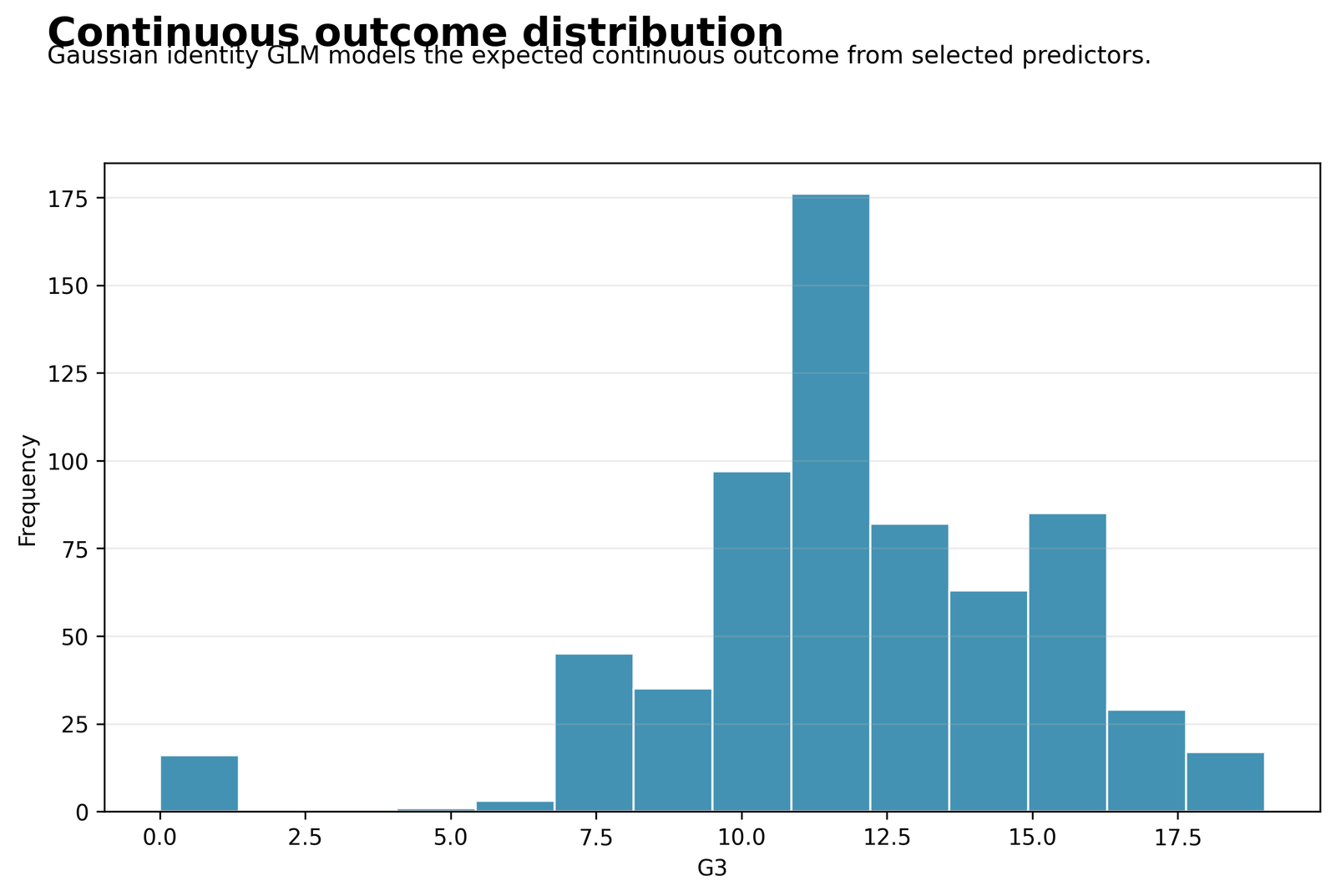
The continuous response is G3, the final grade. All 649 students are used. G3 ranges from 0 to 19, with a mean of approximately 11.906 and a standard deviation of about 3.231. Most scores lie between roughly 8 and 16, while a small group has G3 = 0. This lower tail is important because it creates the most extreme negative residuals in the Gaussian model.
The chart establishes that the Gaussian identity model predicts G3 on its original grade scale. It does not require converting grades into categories. The main fitted model has deviance 1002.1000, Pearson χ² 1002.1000, scale 1.5707, AIC 2145.7210, and log likelihood −1061.8605.
Python Chart 2: Gaussian GLM Observed vs Fitted Values
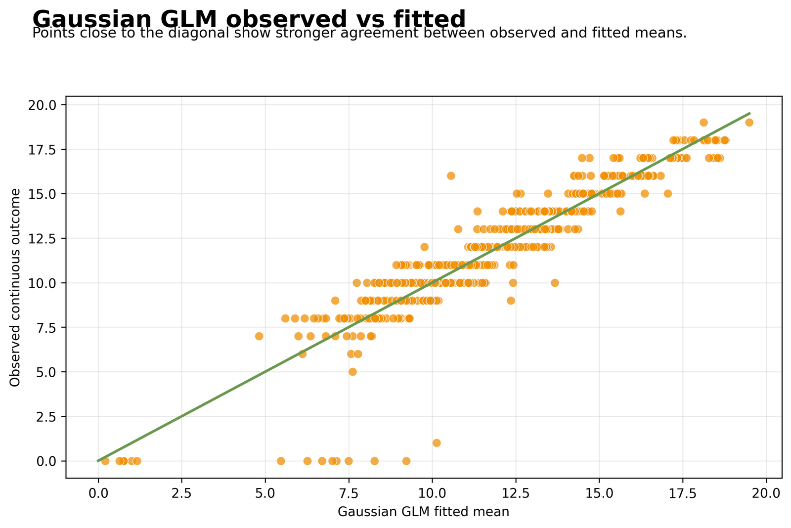
The observed-versus-fitted plot compares each student’s observed G3 with the Gaussian GLM fitted mean. Most of the 649 points lie near the diagonal between fitted values of approximately 7 and 19. The horizontal bands occur because G3 is integer-valued, whereas fitted means are continuous.
The largest discrepancies occur among students whose observed G3 is 0 but whose fitted value is between approximately 5 and 10. The model nevertheless fits the central academic range closely because G2 has B = 0.8804 and G1 has B = 0.1295. Holding the remaining predictors constant, each additional G2 point is associated with about 0.880 additional G3 points, and each G1 point with about 0.130 additional G3 points.
Python Chart 3: Gaussian GLM Residuals vs Fitted Values
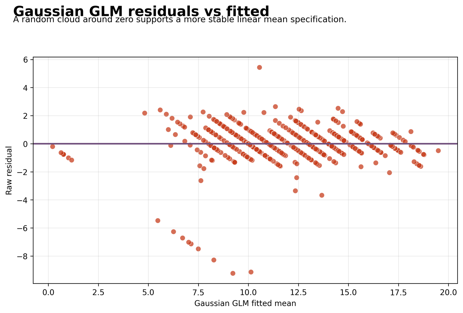
Residuals are calculated as observed G3 minus the Gaussian fitted mean. Most residuals lie between approximately −2 and +2.5 around zero. The diagonal stripes are caused by the integer outcome and are not automatically evidence of model failure.
Several extreme negative residuals reach approximately −9.3, while the largest positive residual is about +5.5. These points represent students whose final grades were substantially lower or higher than predicted from G1, G2, studytime, failures, age, Medu, Fedu, school, sex and address. The model’s Gaussian scale is 1.5707, implying a residual standard deviation of roughly 1.253.
The broad cloud is reasonably centered, but the extreme tail should be checked with studentized residuals, Cook’s distance, Mahalanobis distance, and influence diagnostics.
Python Chart 4: Binomial GLM Probability Calibration
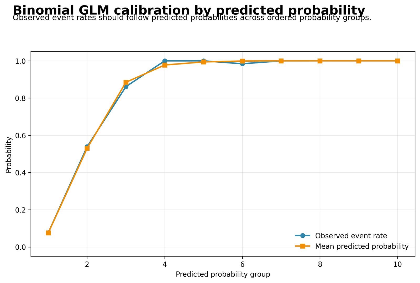
The binomial outcome is glm_pass, coded 1 when G3 ≥ 10 and 0 otherwise. The calibration plot groups predicted probabilities and compares each group’s mean predicted probability with its observed pass rate. Points close to the diagonal indicate agreement between predicted and observed event frequencies.
The fitted binomial model has deviance 176.1896, Pearson χ² 1327.5772, AIC 198.1896, and log likelihood −88.0948. The large Pearson statistic relative to 638 residual degrees of freedom suggests overdispersion or lack of fit that deserves attention even when discrimination is strong.
The coefficient scale is log odds. For example, the fitted G1 and G2 terms should be exponentiated to obtain odds ratios. The calibration chart must be interpreted together with classification, ROC, and dispersion diagnostics rather than used alone.
Python Chart 5: Poisson GLM Observed vs Fitted Counts
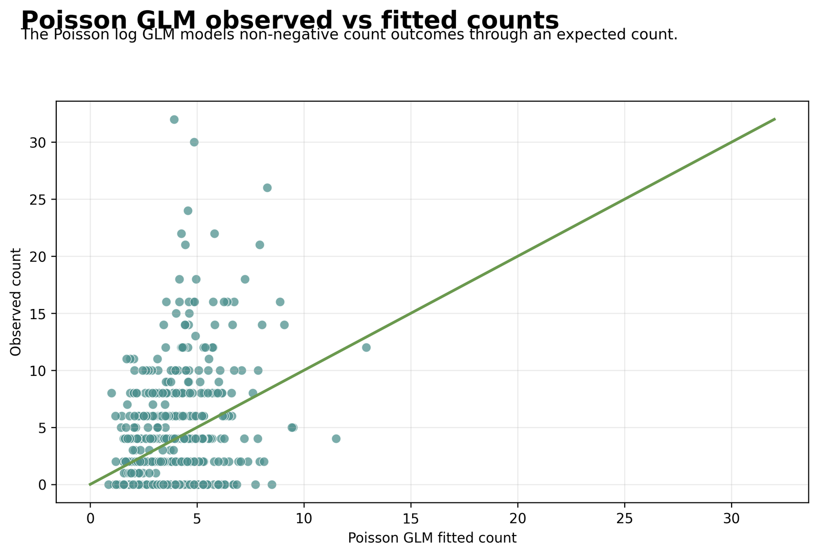
The Poisson outcome is glm_count, created by rounding absences and clipping negative values at zero. The observed-versus-fitted chart shows that fitted Poisson means are compressed relative to the wide observed count range. Many students have low counts, but several observed absence counts are much larger than their predicted values.
The Poisson model has deviance 3067.1642 and Pearson χ² 3161.2421 with 638 residual degrees of freedom. The Pearson dispersion ratio is therefore approximately 3161.2421 / 638 = 4.9549, far above 1. This is strong evidence of overdispersion. The Poisson AIC is 4462.2974 and log likelihood is −2220.1487.
Because the variance greatly exceeds the mean assumption of Poisson regression, a negative-binomial or quasi-Poisson model may be more appropriate. The coefficient scale is the log count rate, and exp(B) is interpreted as a rate ratio.
Python Chart 6: Gaussian GLM Coefficients with 95% Confidence Intervals
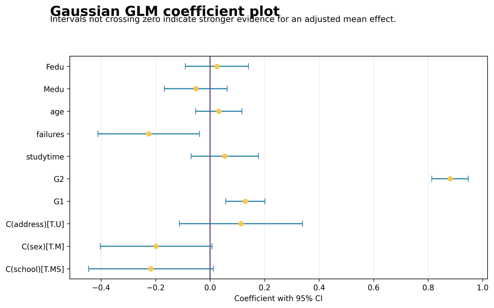
The Gaussian coefficient plot displays adjusted mean effects and 95% confidence intervals. Three predictors are statistically significant at α = .05. G1 has B = 0.1295, SE = 0.0368, p = .0004, CI [0.0575, 0.2016]. G2 has B = 0.8804, SE = 0.0343, p < .001, CI [0.8131, 0.9477]. failures has B = −0.2253, SE = 0.0951, p = .0179, CI [−0.4118, −0.0389].
School_MS, sex_M, address_U, studytime, age, Medu and Fedu have intervals crossing zero. School_MS is close to significance, B = −0.2170, p = .0629; sex_M is also close, B = −0.1981, p = .0583. These should be described as non-significant at .05 rather than significant trends.
Python Chart 7: AIC Summary Across Gaussian, Binomial and Poisson GLMs
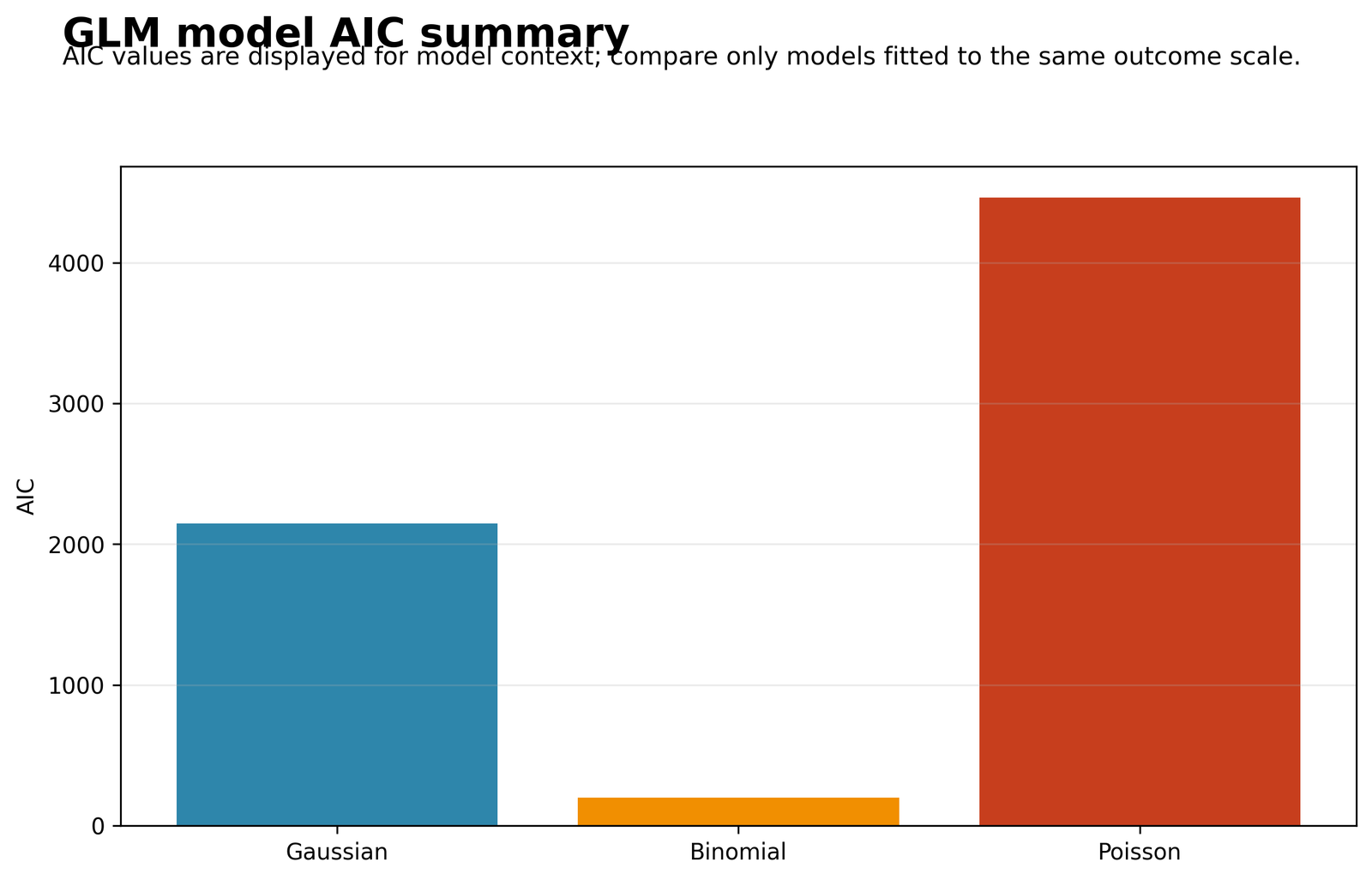
The AIC chart places the three model AIC values side by side: 198.1896 for the binomial logit model, 2145.7210 for the Gaussian identity model, and 4462.2974 for the Poisson log model. These bars should not be used to choose one outcome model over another because the models use different response variables and likelihood scales.
AIC is meaningful only when models are fitted to the same outcome and data. The chart is therefore a summary of each fitted model’s own information criterion, not proof that the binomial model is universally superior. Valid comparisons would involve alternative binomial specifications for glm_pass, alternative Gaussian specifications for G3, or Poisson versus negative-binomial specifications for glm_count.
Binomial Calibration and Poisson Overdispersion Interpretation
Calibration, Discrimination and Classification
Calibration asks whether predicted probabilities agree with observed event frequencies. Discrimination asks whether higher-risk students receive larger predicted probabilities than lower-risk students. Classification applies a threshold to turn probabilities into predicted classes.
The supplied calibration chart groups predicted probabilities and compares them with observed pass rates. A model can calibrate well but discriminate poorly, or discriminate well while probabilities are systematically too high or too low. Therefore, report grouped calibration, calibration slope and intercept when available, ROC AUC, sensitivity, specificity, precision and the threshold-selection rule.
Because most students pass under the G3 ≥ 10 definition, overall accuracy alone may be misleading. A classifier that predicts pass for nearly everyone can achieve high accuracy while failing to identify the non-pass group.
Dispersion Diagnostics
Dispersion compares observed residual variation with the variance expected by the family. For the binomial model, Pearson χ² divided by 638 residual degrees of freedom is approximately 2.0808. For the Poisson model, the ratio is approximately 4.9549.
A ratio near one supports the theoretical variance. Ratios substantially above one indicate extra variation, omitted structure, influential observations, dependence or an unsuitable family. Binomial overdispersion may arise from unmodeled heterogeneity or clustering. Poisson overdispersion is common when counts have a long upper tail.
Robust standard errors can protect inference against some variance misspecification, but they do not change fitted means. Negative-binomial regression changes the count variance model, while quasi-Poisson estimates a dispersion multiplier. Hurdle and zero-inflated models address separate zero-generating mechanisms rather than overdispersion in general.
Count-Model Alternatives
Quasi-likelihood methods specify the mean–variance relationship without requiring a complete response likelihood. Quasi-Poisson keeps the Poisson log mean but estimates a dispersion parameter, inflating standard errors when variance exceeds the mean. This directly addresses the observed dispersion ratio near 4.95.
Because quasi-Poisson does not use a full likelihood, it does not provide a conventional AIC. Negative-binomial regression does use a likelihood and is therefore suitable when AIC-based comparison is needed. Robust sandwich covariance is another option for protecting standard errors, although it does not change fitted Poisson means or solve severe mean misspecification.
The choice among Poisson, quasi-Poisson and negative binomial should consider dispersion, zero frequency, residual shape, prediction and scientific interpretation. A hurdle or zero-inflated model is only justified when a distinct zero-generating mechanism is plausible.
R Generalized Linear Model Design and Reproduction Workflow
R reproduces the same three formulas with glm(). The data must use the same 649 rows, the same derived outcomes, the same predictor coding and the same reference groups. Gaussian uses gaussian(link = "identity"), binomial uses binomial(link = "logit"), and Poisson uses poisson(link = "log").
No complete hosted R report was supplied with the GLM media. The post therefore does not invent an R PDF or pretend that duplicated Python image URLs are independent R charts. The R section provides exact reproduction instructions and includes only the two distinct R-specific chart exports actually supplied.
| R Outcome | Creation | Model Call |
|---|---|---|
| G3 | Use original continuous final grade. | glm(..., family = gaussian(link="identity")) |
| glm_pass | as.integer(G3 >= 10) | glm(..., family = binomial(link="logit")) |
| glm_count | Round absences and keep nonnegative. | glm(..., family = poisson(link="log")) |
R GLM Verification Results and Cross-Software Checks
When R is fitted with identical data and coding, its maximum-likelihood results should agree with the verified Python benchmark to ordinary rounding tolerance. The following values are validation targets, not fabricated results from a missing R report.
| Verification Target | Gaussian | Binomial | Poisson |
|---|---|---|---|
| N | 649 | 649 | 649 |
| Deviance | 1002.1000 | 176.1896 | 3067.1642 |
| Pearson χ² | 1002.1000 | 1327.5772 | 3161.2421 |
| AIC | 2145.7210 | 198.1896 | 4462.2974 |
| Log likelihood | −1061.8605 | −88.0948 | −2220.1487 |
| Dispersion diagnostic | 1.5707 | 2.0808 | 4.9549 |
Reproducibility Requirements
Equivalent GLM results require identical rows, outcome coding, predictor coding, categorical reference groups, family, link, convergence criteria and covariance type. Small differences can arise from how software handles categorical contrasts, missing values, dispersion and confidence intervals.
Python and R should reproduce the same maximum-likelihood estimates when the formula and data are identical. SPSS GENLIN may display Wald statistics and fit measures with different rounding. Excel can reproduce fitted values once coefficients are supplied, but the worked workbook is not a replacement for IRLS estimation.
Every published workflow should state the formula explicitly. For this article, the Gaussian, binomial and Poisson formulas use the same predictors, but the response transformation and link change. Keeping those distinctions visible prevents accidental mixing of odds-ratio, rate-ratio and mean-difference interpretations.
R-Specific GLM Chart Exports with Real Values
Only two distinct R-specific image exports were supplied. Repeated URLs for the outcome distribution, observed-versus-fitted, residual, calibration and Poisson count charts are identical to the Python files and are not embedded again.
R Chart 1: Gaussian GLM Coefficients with 95% Confidence Intervals
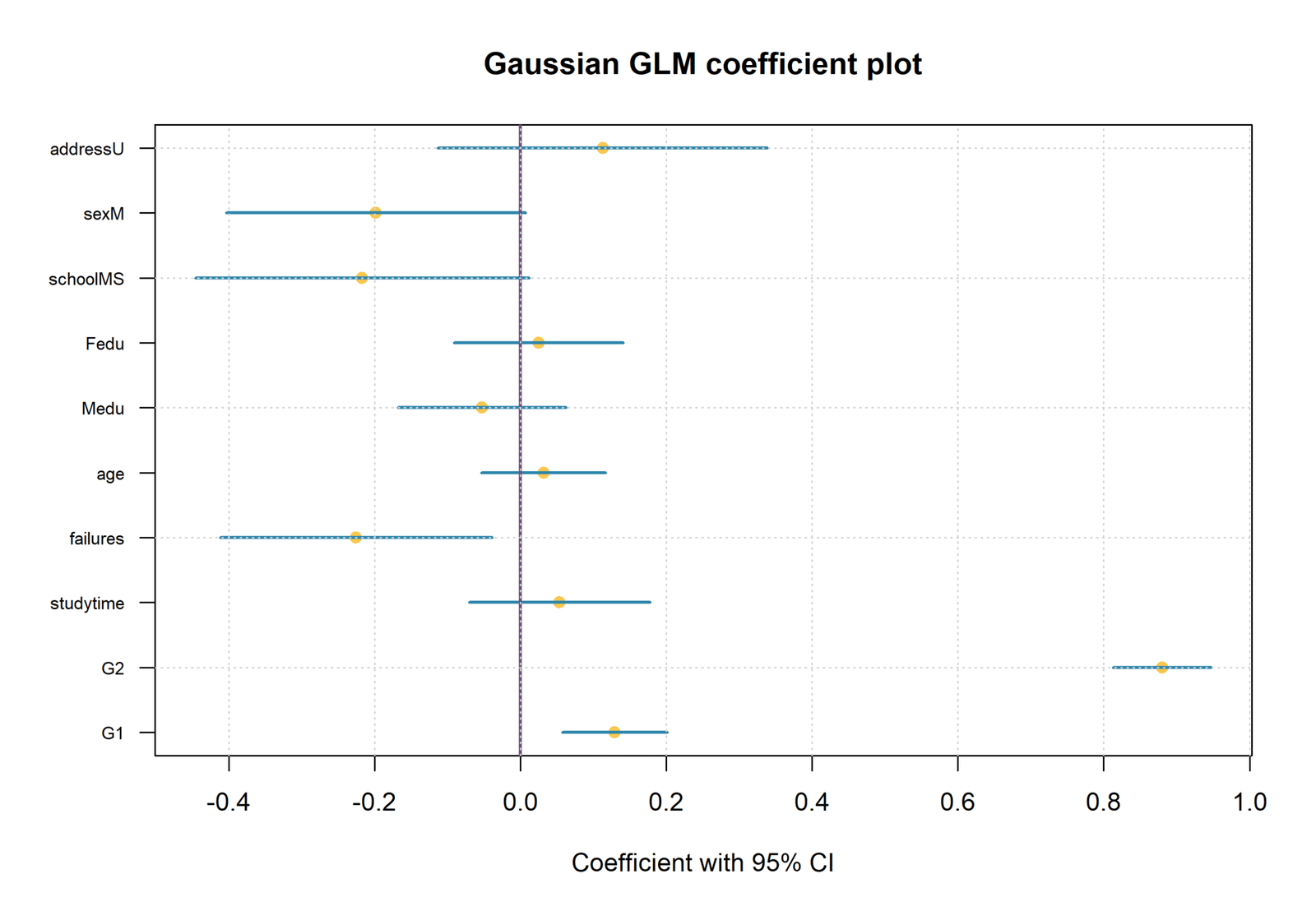
The R coefficient export reproduces the verified Gaussian pattern. G2 = 0.8804 with 95% CI [0.8131, 0.9477], G1 = 0.1295 with CI [0.0575, 0.2016], and failures = −0.2253 with CI [−0.4118, −0.0389]. These three intervals exclude zero.
School_MS, sex_M, address_U, studytime, age, Medu and Fedu have intervals crossing zero. School_MS has B = −0.2170, p = .0629, and sex_M has B = −0.1981, p = .0583. They are close to the threshold but remain non-significant at α = .05.
R Chart 2: Gaussian, Binomial and Poisson AIC Summary
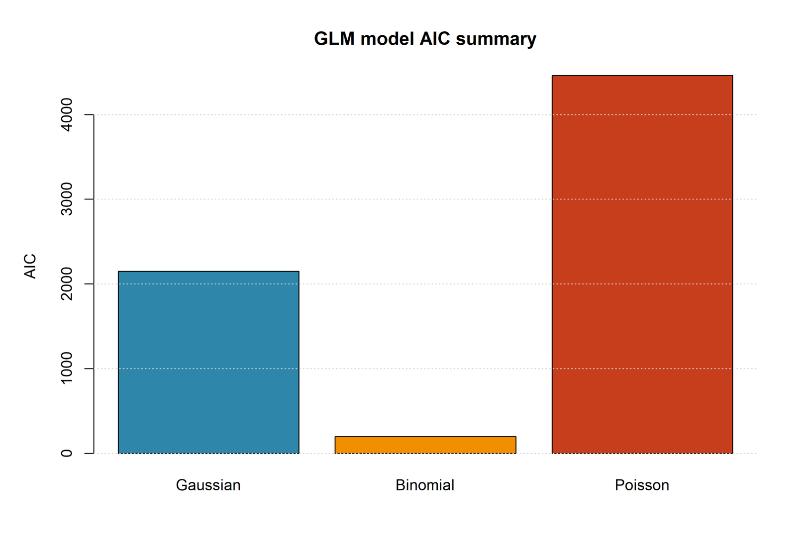
The chart displays AIC values of 2145.7210 for Gaussian, 198.1896 for binomial and 4462.2974 for Poisson. The bars cannot be used to select one universal winner because the outcome variables and likelihood scales differ.
Valid AIC comparisons require the same response and the same observations. Compare Gaussian alternatives for G3, binomial alternatives for glm_pass, or full-likelihood count alternatives for glm_count.
How to Choose the Correct GLM Family and Model
Likelihood-ratio tests, AIC and BIC comparisons require compatible models. The observations and outcome should be the same, and one should understand whether the models are nested. Comparing Gaussian G3 AIC with binomial pass AIC is invalid because the likelihoods represent different outcomes.
Within the Poisson outcome, it is reasonable to compare alternative predictor sets, interactions or links when likelihood assumptions permit. Negative-binomial AIC may be compared with Poisson AIC if both are estimated by full likelihood on the same count outcome. Quasi-Poisson does not provide a conventional likelihood AIC.
Outcome-Driven Selection
| Research Goal | Outcome | Recommended Starting Model |
|---|---|---|
| Predict expected final grade | Continuous G3 | Gaussian identity GLM. |
| Predict probability of passing | Binary glm_pass | Binomial logit GLM. |
| Predict expected absences | Count glm_count | Poisson log GLM, followed by dispersion assessment. |
| Model smooth nonlinear effects | Any supported outcome | Generalized additive model. |
| Account for correlated clusters | Repeated or clustered outcome | GEE or generalized mixed model. |
The fitted coefficients describe adjusted associations in an observational student dataset. They do not prove that changing G1, G2, studytime, school or any background variable causes a change in G3, pass status or absences. Causal interpretation requires a defensible design, temporal ordering, confounding assumptions and appropriate sensitivity analysis.
G1 and G2 are previous grades measured before G3 and therefore have a plausible predictive role, but they may also summarize many prior influences. Group coefficients for school, sex and address should be interpreted as adjusted differences under the model, not as inherent characteristics or policy effects.
The models are most defensible as explanatory and predictive summaries of the analyzed sample. External validation is required before applying their numerical predictions to a different school system, cohort or grading policy.
Dispersion, Exposure and Count-Model Issues
Dispersion compares observed residual variation with the variance expected by the family. For the binomial model, Pearson χ² divided by 638 residual degrees of freedom is approximately 2.0808. For the Poisson model, the ratio is approximately 4.9549.
A ratio near one supports the theoretical variance. Ratios substantially above one indicate extra variation, omitted structure, influential observations, dependence or an unsuitable family. Binomial overdispersion may arise from unmodeled heterogeneity or clustering. Poisson overdispersion is common when counts have a long upper tail.
Robust standard errors can protect inference against some variance misspecification, but they do not change fitted means. Negative-binomial regression changes the count variance model, while quasi-Poisson estimates a dispersion multiplier. Hurdle and zero-inflated models address separate zero-generating mechanisms rather than overdispersion in general.
Offsets and Exposure
Count outcomes often depend on how long each observation was at risk. A person observed for twelve months has more opportunity to accumulate events than a person observed for three months. A Poisson or negative-binomial model handles unequal exposure by adding the logarithm of exposure as an offset with its coefficient fixed at one.
The resulting exponentiated coefficients are rate ratios rather than simple count ratios. In the current student-absence example, every student is assumed to represent a comparable school period, so no offset is used. If enrollment duration, attendance eligibility or observation time differed, ignoring exposure would make fitted rates incomparable.
Quasi-Likelihood and Robust Alternatives
Quasi-likelihood methods specify the mean–variance relationship without requiring a complete response likelihood. Quasi-Poisson keeps the Poisson log mean but estimates a dispersion parameter, inflating standard errors when variance exceeds the mean. This directly addresses the observed dispersion ratio near 4.95.
Because quasi-Poisson does not use a full likelihood, it does not provide a conventional AIC. Negative-binomial regression does use a likelihood and is therefore suitable when AIC-based comparison is needed. Robust sandwich covariance is another option for protecting standard errors, although it does not change fitted Poisson means or solve severe mean misspecification.
The choice among Poisson, quasi-Poisson and negative binomial should consider dispersion, zero frequency, residual shape, prediction and scientific interpretation. A hurdle or zero-inflated model is only justified when a distinct zero-generating mechanism is plausible.
The present absence count assumes a comparable observation period for every student. If students were observed for different durations, the logarithm of exposure should enter as an offset with coefficient fixed at one.
GLM Residuals, Influence and Diagnostic Checks
| Family | Primary Diagnostics | Main Warning in This Example |
|---|---|---|
| Gaussian | Residual vs fitted, Q–Q plot, influence, variance pattern | Extreme negative residuals. |
| Binomial | Calibration, ROC, classification, deviance residuals, separation | Large Pearson statistic. |
| Poisson | Dispersion, zeros, residuals, observed vs fitted counts | Dispersion ratio about 4.95. |
Useful internal diagnostic guides include Q–Q plots, outlier detection, VIF and tolerance.
Influence and Leverage
Leverage measures how unusual an observation’s predictor pattern is. Influence measures how much the fitted model changes when an observation is removed or down-weighted. A case can have a large residual but low leverage, or high leverage but a small residual. The most influential cases combine unusual predictors with poor fit.
The Gaussian residual chart contains several students with observed G3 = 0 but fitted values around 6 to 10. Their influence depends on whether their G1, G2 and other predictors are also unusual. Use Cook’s distance, Mahalanobis distance and influence diagnostics.
Influential observations should be investigated for data-entry errors, unusual circumstances and scientific plausibility. Report sensitivity analyses when important conclusions change after an influential case is excluded. Do not silently delete observations to improve model fit.
Validation and Generalization
The supplied report focuses on full-sample fitted models. Fitted residuals and AIC describe the analyzed data but do not directly estimate performance in new observations. For prediction, use train/test evaluation, k-fold cross-validation or bootstrap validation.
All preprocessing must occur inside the training folds. This includes dummy coding, transformations, predictor selection and threshold choices. For binomial classification, select cutoffs using training or validation data rather than optimizing them on the final test set.
External validation is required before applying the model to students from another school system, later cohort or different grading environment. Differences in grade distributions, absence recording and educational policies can change calibration and coefficient values.
Interpretive and Causal Limits
The fitted coefficients describe adjusted associations in an observational student dataset. They do not prove that changing G1, G2, studytime, school or any background variable causes a change in G3, pass status or absences. Causal interpretation requires a defensible design, temporal ordering, confounding assumptions and appropriate sensitivity analysis.
G1 and G2 are previous grades measured before G3 and therefore have a plausible predictive role, but they may also summarize many prior influences. Group coefficients for school, sex and address should be interpreted as adjusted differences under the model, not as inherent characteristics or policy effects.
The models are most defensible as explanatory and predictive summaries of the analyzed sample. External validation is required before applying their numerical predictions to a different school system, cohort or grading policy.
Worked Excel File for Generalized Linear Models
The hosted workbook contains Gaussian_GLM, Binomial_GLM, Poisson_GLM and Reporting_Guide sheets. It demonstrates formulas rather than estimating coefficients through IRLS.
Download the worked GLM Excel file
Gaussian worked example
The illustrative coefficients are intercept 1.50, G1 0.12, G2 0.72, studytime 0.25, failures −0.85 and absences −0.03. Across 20 example rows, mean observed G3 is 11.60, RMSE 1.0555 and MAE 0.8415.
Binomial worked example
The example event rate is 0.75, mean predicted probability 0.5608 and classification accuracy 0.85. Probability is calculated as 1/(1+EXP(−η)).
Poisson worked example
The illustrative mean observed count is 4.35, mean fitted count 1.8903 and RMSE 3.5572. The large underprediction demonstrates why the count model needs careful fit assessment.
Gaussian fitted mean:
=Intercept+B1*G1+B2*G2+...

Binomial probability:
=1/(1+EXP(-Eta))

Poisson fitted count:
=EXP(Eta)

Odds ratio or rate ratio:
=EXP(Coefficient)
Reporting Guide Included in the Workbook
The workbook’s Reporting_Guide sheet states that Gaussian results require coefficients, standard errors, 95% confidence intervals, p-values, fitted means and residual patterns. Binomial results require odds ratios, confidence intervals, predicted probabilities and classification context. Poisson results require rate ratios, fitted counts and explicit dispersion assessment.
Excel limitation: the workbook demonstrates prediction equations and interpretation. It does not replace the iterative maximum-likelihood fitting performed by Python, R or SPSS.
SPSS Generalized Linear Model Workflow
Use GENLIN and specify the outcome distribution and link separately for each model. Do not use one output interpretation across all families.
GENLIN G3 BY school sex address
  WITH G1 G2 studytime failures age Medu Fedu
  /MODEL G1 G2 studytime failures age Medu Fedu school sex address
    DISTRIBUTION=NORMAL LINK=IDENTITY
  /PRINT MODELINFO FIT SUMMARY SOLUTION.

GENLIN glm_pass BY school sex address
  WITH G1 G2 studytime failures age Medu Fedu
  /MODEL G1 G2 studytime failures age Medu Fedu school sex address
    DISTRIBUTION=BINOMIAL LINK=LOGIT
  /PRINT MODELINFO FIT SUMMARY SOLUTION.

GENLIN glm_count BY school sex address
  WITH G1 G2 studytime failures age Medu Fedu
  /MODEL G1 G2 studytime failures age Medu Fedu school sex address
    DISTRIBUTION=POISSON LINK=LOG
  /PRINT MODELINFO FIT SUMMARY SOLUTION.
No GLM-specific SPSS PDF URL was supplied with the current media. The workflow is included without inventing a download or unsupported SPSS coefficient table.
Python, R and SPSS Code for Generalized Linear Models
# Python
gaussian = smf.glm(formula_gaussian, data=df,
    family=sm.families.Gaussian(sm.families.links.Identity())).fit()
binomial = smf.glm(formula_binomial, data=df,
    family=sm.families.Binomial(sm.families.links.Logit())).fit()
poisson = smf.glm(formula_poisson, data=df,
    family=sm.families.Poisson(sm.families.links.Log())).fit()
# R
gaussian <- glm(G3 ~ G1 + G2 + studytime + failures + age +
Medu + Fedu + school + sex + address,
data=df, family=gaussian(link="identity"))
binomial <- glm(glm_pass ~ G1 + G2 + studytime + failures + age +
Medu + Fedu + school + sex + address,
data=df, family=binomial(link="logit"))
poisson <- glm(glm_count ~ G1 + G2 + studytime + failures + age +
Medu + Fedu + school + sex + address,
data=df, family=poisson(link="log"))R Reproduction Code
df <- read.csv("dataset.csv")
df$glm_pass <- as.integer(df$G3 >= 10)
df$glm_count <- pmax(round(df$absences), 0)

gaussian_model <- glm(
  G3 ~ G1 + G2 + studytime + failures + age +
    Medu + Fedu + school + sex + address,
  data = df,
  family = gaussian(link = "identity")
)

binomial_model <- glm(
  glm_pass ~ G1 + G2 + studytime + failures + age +
    Medu + Fedu + school + sex + address,
  data = df,
  family = binomial(link = "logit")
)

poisson_model <- glm(
  glm_count ~ G1 + G2 + studytime + failures + age +
    Medu + Fedu + school + sex + address,
  data = df,
  family = poisson(link = "log")
)

summary(gaussian_model)
summary(binomial_model)
summary(poisson_model)

deviance(poisson_model)
sum(residuals(poisson_model, type = "pearson")^2) /
  df.residual(poisson_model)
APA-Style Reporting for Generalized Linear Models
| Item | What to State |
|---|---|
| Outcome | Name, scale and coding of G3, glm_pass or glm_count. |
| Family and link | Gaussian identity, binomial logit or Poisson log. |
| Sample | N = 649 and any exclusion criteria. |
| Predictors | Exact variable names and categorical reference groups. |
| Fit | Deviance, Pearson chi-square, scale, AIC and log likelihood as appropriate. |
| Effects | B, SE, confidence interval, p-value and exp(B) where relevant. |
| Diagnostics | Residual patterns, calibration, dispersion and influence. |
| Validation | Held-out or cross-validated performance when prediction is claimed. |
| Limitations | Overdispersion, imbalance, nonlinearity, missingness and generalizability. |
A Gaussian identity-link generalized linear model was fitted to predict G3 from academic and demographic predictors for 649 students. G1, B = 0.130, SE = 0.037, p < .001, G2, B = 0.880, SE = 0.034, p < .001, and failures, B = −0.225, SE = 0.095, p = .018, were significant. The model had deviance = 1002.10 and AIC = 2145.72.
A binomial logit GLM predicted glm_pass, coded 1 when G3 ≥ 10. Model deviance was 176.19 and AIC was 198.19. Coefficients were interpreted as log odds and exponentiated to obtain odds ratios. Calibration and the large Pearson χ² were considered when assessing fit.
A Poisson log GLM predicted rounded absence counts. The Pearson dispersion ratio was approximately 4.95, indicating substantial overdispersion; therefore, Poisson standard errors require caution and an alternative count model should be considered.
Cross-Software Reporting
Equivalent GLM results require identical rows, outcome coding, predictor coding, categorical reference groups, family, link, convergence criteria and covariance type. Small differences can arise from how software handles categorical contrasts, missing values, dispersion and confidence intervals.
Python and R should reproduce the same maximum-likelihood estimates when the formula and data are identical. SPSS GENLIN may display Wald statistics and fit measures with different rounding. Excel can reproduce fitted values once coefficients are supplied, but the worked workbook is not a replacement for IRLS estimation.
Every published workflow should state the formula explicitly. For this article, the Gaussian, binomial and Poisson formulas use the same predictors, but the response transformation and link change. Keeping those distinctions visible prevents accidental mixing of odds-ratio, rate-ratio and mean-difference interpretations.
Common Generalized Linear Model Mistakes
| Mistake | Correction |
|---|---|
| Not naming outcome variables | State G3, glm_pass and glm_count with coding. |
| Interpreting all coefficients as mean differences | Use mean difference, odds ratio or rate ratio according to link. |
| Comparing AIC across different outcomes | Compare AIC only for models fitted to the same outcome. |
| Ignoring Poisson overdispersion | Report Pearson dispersion and consider negative binomial. |
| Using calibration alone | Add discrimination and classification for binomial models. |
| Calling non-significant terms significant | School and sex Gaussian p-values exceed .05. |
Most important correction: never compare the Gaussian, binomial and Poisson AIC bars as though they were alternative models for the same outcome. Their responses and likelihood scales differ.
Generalized Linear Model Downloads
Gaussian, binomial and Poisson results with seven charts.Worked Excel File
Formula-based Gaussian, binomial and Poisson examples.
No complete R report or SPSS report URL was supplied, so only the verified Python PDF and hosted Excel workbook are included as downloads.
FAQs About Generalized Linear Models
What is a GLM?
A GLM combines an outcome family, a linear predictor and a link function.
What are the three outcomes here?
G3, glm_pass and glm_count.
Which Gaussian predictors are significant?
G1, G2 and failures.
How is glm_pass coded?
1 when G3 ≥ 10 and 0 otherwise.
How is glm_count created?
Rounded absences clipped at zero.
What does exp(B) mean in binomial GLM?
An odds ratio.
What does exp(B) mean in Poisson GLM?
A rate ratio.
Is the Poisson model overdispersed?
Yes. Pearson χ² divided by residual df is about 4.95.
Can AIC be compared across these three outcomes?
No. AIC comparisons require the same response and data.
Can Excel estimate GLM coefficients?
The workbook demonstrates formulas; Python, R or SPSS should perform IRLS estimation.

