
Relative Risk: Formula, Calculation, Interpretation, Calculator, Python, R, SPSS, SAS and Excel Guide
This Relative Risk guide analyses 649 student records rather than relying on a generic example. The event is a final grade of at least 10. MS recorded 158 passes among 226 students, while GP recorded 391 passes among 423 students. The complete analysis reports the exact 2 × 2 table, group risks, relative risk, confidence interval, absolute difference, complementary failure-risk result, software calculations, chart evidence and reporting language.
Relative Risk Model Overview
Relative risk, also called the risk ratio, compares the probability of an event in one group with the probability of the same event in a reference group. It is calculated from group-specific denominators, not from the total sample and not from odds. In the worked data, MS is the comparison group, GP is the reference group, and the event is G3 ≥ 10.
The analysis begins with the observed counts. MS has 158 passes and 68 failures, for a pass risk of 69.91%. GP has 391 passes and 32 failures, for a pass risk of 92.43%. Dividing the two risks gives RR = 0.756332. This means the observed probability of passing in MS is 75.63% of the probability in GP. Equivalently, the MS pass probability is 24.37% lower on the relative scale.
The Exact Data Question
How does the probability of obtaining G3 ≥ 10 in MS compare with the probability in GP, and how precisely is that comparison estimated?
What the Observed Data Show Before Any Formula
Different Denominators
GP contains 423 students and MS contains 226. A simple comparison of 391 passes with 158 passes would therefore mix group size with outcome probability. Converting each count to a within-school risk removes that denominator imbalance.
Different Outcome Mixes
GP records 391 passes and 32 failures, so failures form only 7.57% of its row. MS records 158 passes and 68 failures, so failures form 30.09% of its row. The ratio analysis summarizes this difference on the pass-probability scale.
Three Numerically Equivalent Ways to State the Main Result
MS pass probability is 0.7563 times GP pass probability.
One minus the ratio gives the relative difference from the GP baseline.
GP pass probability is 1.3222 times the MS pass probability.
These statements are algebraically connected, but they are not interchangeable in wording. The first preserves the selected MS/GP direction. The second expresses distance below the reference as a percentage. The reciprocal reverses the comparison and must explicitly name GP as the numerator.
Quick Answer: Relative Risk Result
The observed pass probability is 69.91% in MS and 92.43% in GP. Their ratio is 0.756332. The confidence interval does not cross the null value of 1, and the absolute risk difference is -22.52%.
Statistical Reading
- Null value: RR = 1
- Observed estimate: RR = 0.756332
- Log standard error: 0.045802
- Wald z: -6.097
- Confidence-interval decision: interval excludes 1
Data Meaning
- MS: 158 of 226 passed.
- GP: 391 of 423 passed.
- MS had 24.37% lower pass risk relatively.
- The absolute pass-rate gap was 22.52%.
- MS had 3.98 times the failure risk of GP.
Table of Contents
- Meaning of relative risk
- Research question and hypotheses
- When to use relative risk
- Risk measures and variants
- Variables and raw-data audit
- Formula and manual calculation
- Observed tables and data patterns
- Complete results
- Assumptions and sensitivity checks
- Comparison with related measures
- Calculator workflow
- Python chart interpretations
- Paired R chart interpretations
- Software workflows
- Expandable code
- Interpretation and APA reporting
- Common mistakes
- Practice questions
- Downloads
- Related guides
- Frequently asked questions
- Conclusion
What Is Relative Risk?
Relative risk is a ratio of two probabilities. The numerator is the event risk in the focal or exposed group, and the denominator is the event risk in the reference or unexposed group. A value of 1 indicates equal observed risks. A value below 1 indicates lower risk in the numerator group. A value above 1 indicates higher risk in the numerator group.
Risk Is Not the Same as a Share of All Events
MS contributed 28.78% of all passes, but that is not the MS pass risk. The correct MS risk is 158 divided by all 226 MS students, which equals 69.91%. GP contributed 71.22% of all passes, but its risk is 391 divided by 423, which equals 92.43%. Relative risk requires these within-group denominators.
The Reference Group Controls the Direction
This post calculates MS divided by GP. Reversing the groups gives 1/RR = 1.3222; that reciprocal says GP has about 1.32 times the pass probability of MS. Both calculations describe the same two risks, but the written interpretation must match the chosen numerator and denominator.
Event Coding Also Controls the Meaning
When “pass” is the event, RR = 0.7563. When “failure” is the event, RR = 3.9773. These are not contradictions. They answer complementary questions: the pass probability is lower in MS, and the failure probability is higher in MS.
Relative Risk Is a Conditional Probability Comparison
The two probabilities are conditional on school membership: P(pass | MS) and P(pass | GP). The vertical bar means “given.” The calculation therefore asks what fraction of students passed within each school, not what fraction of the total sample belonged to each school. This conditional structure is the defining feature of relative risk.
Why the Baseline Risk Must Be Printed
A relative risk of 0.7563 cannot be interpreted fully without the GP baseline of 92.43%. Applying the same ratio to a baseline of 10% would imply 7.56%, an absolute gap of only 2.44 percentage points. Here the high GP baseline converts the same ratio into a much larger 22.52-point absolute gap. This is why responsible reporting displays both group risks beside the ratio.
Risk, Rate and Odds Are Different Quantities
The current denominator is the number of students in each school, so the result is a risk or proportion. A rate would require person-time, such as student-years of observation. Odds divide events by non-events: MS pass odds are 158/68, whereas MS pass risk is 158/226. The distinction explains why the odds ratio is 0.1902 while the risk ratio is 0.7563.
Research Question, Hypotheses and Data Design
Research Question
Among the 649 observed students, how does the probability of G3 ≥ 10 in MS compare with the probability in GP?
Null and Alternative Hypotheses
| Component | Expression | Data meaning |
|---|---|---|
| Null hypothesis | H0: RR = 1 | MS and GP have equal pass probabilities. |
| Two-sided alternative | H1: RR ≠ 1 | The pass probabilities differ. |
| Observed direction | RR < 1 | MS has the lower observed pass probability. |
| Confidence-interval rule | Reject equality when the 95% CI excludes 1 | The current interval is entirely below 1. |
Design Statement
This is an independent two-group comparison based on school membership and a binary outcome derived from G3. It is not a matched design, repeated-measures design or randomized intervention. Each student contributes once to one school row and one pass/fail column.
Unit of Analysis and Estimand
The unit of analysis is one student record. The estimand is the unadjusted ratio of the two observed pass probabilities. It does not average school-specific effects across another stratifier, estimate an individual treatment effect or model the full G3 scale. Stating the estimand prevents the analysis from being confused with a mean comparison or an adjusted regression coefficient.
Why the Hypothesis Is About a Ratio
Equality of risks means 158/226 and 391/423 estimate the same underlying probability. On the ratio scale, equality becomes RR = 1. On the log scale used for the confidence interval, equality becomes ln(RR) = 0. The observed ln(RR) is −0.2793, so the estimate lies below both null representations.
When to Use Relative Risk
Use Relative Risk When
- The outcome is binary.
- Both group denominators are observed.
- Each observation belongs to one independent group.
- The event probability is directly estimable.
- A ratio of probabilities is scientifically meaningful.
- Cohort, trial or complete cross-sectional counts are available.
- The reference group is clearly defined.
- The event direction is fixed before interpretation.
Use Another Method When
- Only case-control sampling fractions are available.
- Observations are matched or repeated.
- Time to event and censoring matter.
- Many covariates require adjusted estimation.
- Survey weights or complex clustering determine precision.
- There are zero cells and an unqualified log interval is unstable.
- The outcome has more than two categories.
- The goal is causal attribution from non-randomized data.
Decision Flow
Use events divided by each group total.
Use relative risk; use risk difference for an absolute gap.
Use log-binomial, robust Poisson or another adjusted model.
In the current data, all four cells are positive and both group denominators are known, so the direct risk-ratio calculation is appropriate as an unadjusted descriptive and inferential comparison.
Why Direct Relative Risk Is Available in This Dataset
Both complete group denominators are present: all 226 MS observations and all 423 GP observations in the workbook. The analysis is not conditioned on a fixed number of passes or failures. Consequently, 158/226 and 391/423 are estimable event probabilities. This denominator information is exactly what is missing in a typical case-control sample, where direct relative risk is usually unavailable.
When an Adjusted Model Would Improve the Analysis
If age, prior grades, attendance, study time or other student characteristics differ between schools, an unadjusted 2 × 2 table may combine school association with compositional differences. A log-binomial model or a Poisson model with robust standard errors can estimate an adjusted risk ratio. The unadjusted table should still be retained because it provides the transparent starting point and a check on model direction.
Relative Risk, Risk Difference and Related Effect Measures
No single effect measure is sufficient for every interpretation. The same observed table can be expressed on relative, absolute, odds and complementary-outcome scales. Reporting the measures together prevents a large-sounding relative statement from hiding the actual event rates.
Probability ratio: 0.7563.
Probability subtraction: -0.2252.
Odds comparison: 0.1902.
Complementary event ratio: 3.9773.
| Measure | Formula from the observed data | Estimate | Correct interpretation |
|---|---|---|---|
| Relative risk | (158/226)/(391/423) | 0.756332 | MS pass risk is 75.63% of GP pass risk. |
| Relative risk reduction | 1 − RR | 0.243668 | MS pass risk is 24.37% lower relatively. |
| Risk difference | 158/226 − 391/423 | -0.225235 | MS has 22.52% fewer passes on the absolute probability scale. |
| Odds ratio | (158×32)/(68×391) | 0.190161 | MS pass odds are 19.02% of GP pass odds. |
| Failure-risk ratio | (68/226)/(32/423) | 3.977323 | MS failure risk is 3.98 times GP failure risk. |
Translate Every Effect Back to the Observed Risks
The relative pass shortfall of 24.37% is calculated against GP’s 92.43% pass risk. Multiplying 92.43% by 24.37% gives the 22.52-percentage-point absolute gap. Conversely, dividing the 22.52-point gap by the 92.43% GP baseline returns 24.37%. This arithmetic link confirms that the relative and absolute summaries describe the same observed table rather than separate findings.
Why the Failure Ratio Is Not the Reciprocal of the Pass Ratio
The reciprocal of the pass RR is 1.3222 because it reverses the groups but retains “pass” as the event. The failure RR of 3.9773 keeps the MS/GP group order but changes the event to failure. Complementing probabilities is not the same operation as inverting a ratio, so these two values should never be substituted for one another.
Variables, Coding and Raw-Data Audit
| Variable | Role | Coding | Valid N | Analytical use |
|---|---|---|---|---|
| school | Group variable | MS or GP | 649 | Defines comparison and reference denominators. |
| G3 | Original numeric outcome | 0 to 19 | 649 | Original final grade retained for audit and threshold analysis. |
| G3 pass | Derived binary event | 1 when G3 ≥ 10; 0 otherwise | 649 | Supplies event and non-event counts for relative risk. |
Group Composition and Grade Distribution
| School | N | Share of sample | Mean G3 | SD | Median | IQR | Range |
|---|---|---|---|---|---|---|---|
| MS | 226 | 34.82% | 10.650 | 3.834 | 11 | 9–13 | 0–19 |
| GP | 423 | 65.18% | 12.577 | 2.626 | 13 | 11–14 | 0–19 |
| Total | 649 | 100.00% | — | — | — | — | 0–19 |
The binary result is consistent with the underlying numeric distribution. GP has a higher mean and median G3, while MS has greater spread. The pass threshold of 10 lies below the GP first quartile of 11 but above the MS first quartile of 9, which helps explain why the binary pass rates separate sharply.
Data Completeness and Coding Audit
| Audit item | Observed result | Why it matters |
|---|---|---|
| Rows represented | 649 | Matches the 2 × 2 table total. |
| School totals | 226 MS; 423 GP | Each record enters one denominator. |
| Event totals | 549 pass; 100 fail | Matches the column totals. |
| Zero cells | None | The ordinary Katz log interval is defined. |
| Threshold | G3 ≥ 10 | The event rule is explicit and reproducible. |
| Direction | MS / GP | All ratio interpretations use the same reference. |
Distributional Evidence Behind the Binary Event
The mean G3 difference is 12.577 − 10.650 = 1.926 points in favor of GP. The medians differ by two grade points, and the interquartile ranges are 11–14 for GP versus 9–13 for MS. MS also has the larger standard deviation, 3.834 compared with 2.626, indicating a wider spread that includes more observations below the pass threshold.
The threshold G3 ≥ 10 converts the numeric outcome into a policy-relevant binary indicator while discarding within-category detail. A student with G3 = 10 and a student with G3 = 19 both count as passes, while G3 = 9 and G3 = 0 both count as failures. The raw-data audit therefore remains necessary even when the target measure is binary.
Sample Balance Does Not Determine the Risk Ratio
GP represents 65.18% of the sample and MS represents 34.82%. Unequal group size affects precision, but it does not invalidate the ratio because each risk uses its own denominator. The smaller MS group contributes most of the log-RR variance, which is examined explicitly in the formula section.
Relative Risk Formula and Manual Calculation
Let a be events in the comparison group, b non-events in the comparison group, c events in the reference group and d non-events in the reference group.
| Symbol | Current value | Definition |
|---|---|---|
| a | 158 | MS passes |
| b | 68 | MS failures |
| c | 391 | GP passes |
| d | 32 | GP failures |
| a+b | 226 | MS total |
| c+d | 423 | GP total |
Step 1: Calculate Each Group Risk
Step 2: Divide the Risks
Step 3: Calculate the Katz Log Standard Error
Step 4: Form the 95% Confidence Interval
Step-by-Step Arithmetic Audit
| Quantity | Substitution | Result |
|---|---|---|
| MS risk | 158 ÷ 226 | 0.699115044 |
| GP risk | 391 ÷ 423 | 0.924349882 |
| Risk ratio | 0.699115044 ÷ 0.924349882 | 0.756331621 |
| Natural log | ln(RR) | -0.279275347 |
| Log SE | Katz formula | 0.045801897 |
| Lower limit | exp[ln(RR) − 1.959964SE] | 0.691394010 |
| Upper limit | exp[ln(RR) + 1.959964SE] | 0.827368349 |
Where the Confidence-Interval Uncertainty Comes From
| Variance component | Formula | Value | Share of log variance |
|---|---|---|---|
| MS contribution | 1/158 − 1/226 | 0.001904335 | 90.78% |
| GP contribution | 1/391 − 1/423 | 0.000193479 | 9.22% |
| Total variance | Sum of components | 0.002097814 | 100.00% |
| Standard error | Square root of total | 0.045801897 | — |
MS contributes about 90.78% of the log-scale variance because it has fewer observations and fewer events than GP. This does not mean MS “causes” the uncertainty; it means the MS risk is estimated less precisely. The Wilson interval width for MS is about 11.88 percentage points compared with 5.08 points for GP.
Why the Ratio Interval Is Asymmetric
The confidence limits are symmetric around ln(RR) on the log scale, not around RR on the original scale. Exponentiation produces a lower distance of 0.0649 and an upper distance of 0.0710 around the point estimate. This asymmetry is expected for a multiplicative measure and should not be “corrected” by forcing equal distances.
Endpoint Interpretation
At the lower endpoint, MS pass risk is 69.14% of GP pass risk, corresponding to a 30.86% relative shortfall. At the upper endpoint, MS pass risk is 82.74% of GP pass risk, corresponding to a 17.26% relative shortfall. Thus, uncertainty changes the magnitude but not the direction of the observed association.
Observed Table, Group Risks and Data Patterns
Observed 2 × 2 Table
| School | Pass: G3 ≥ 10 | Fail: G3 < 10 | Row total |
|---|---|---|---|
| MS | 158 | 68 | 226 |
| GP | 391 | 32 | 423 |
| Column total | 549 | 100 | 649 |
Within-School Percentages
| School | Pass risk | Failure risk | Passes per 1,000 | Failures per 1,000 |
|---|---|---|---|---|
| MS | 69.91% | 30.09% | 699.1 | 300.9 |
| GP | 92.43% | 7.57% | 924.3 | 75.7 |
Contribution to All Outcomes
| Outcome | MS count | GP count | Total | MS share of outcome | GP share of outcome |
|---|---|---|---|---|---|
| Pass | 158 | 391 | 549 | 28.78% | 71.22% |
| Fail | 68 | 32 | 100 | 68.00% | 32.00% |
MS contains only 34.82% of the full sample but contributes 68.00% of all failures. GP contains 65.18% of the sample and contributes 71.22% of all passes. These column shares are descriptive; the relative-risk denominator remains the school total.
Counts Near the Pass Threshold
| G3 score | MS count | GP count | Status under G3 ≥ 10 |
|---|---|---|---|
| 7 | 7 | 3 | Fail |
| 8 | 21 | 14 | Fail |
| 9 | 25 | 10 | Fail |
| 10 | 44 | 53 | Pass |
| 11 | 34 | 70 | Pass |
| 12 | 17 | 55 | Pass |
The threshold neighborhood shows why the event definition matters. MS has 53 students at scores 8 or 9 compared with 24 in GP, while GP has 178 students at 10–12 compared with 95 in MS. The pass-rate difference is therefore supported by the raw score distribution rather than a single isolated cell.
Counterfactual Count Benchmark
| Benchmark | Calculation | Count |
|---|---|---|
| Expected MS passes if MS had GP risk | 226 × 0.924349882 | 208.903 |
| Observed MS passes | Given table | 158 |
| Descriptive pass shortfall | 208.903 − 158 | 50.903 |
Observed Versus Independence Benchmarks
| Cell | Observed | Expected | Observed − expected | Pearson residual |
|---|---|---|---|---|
| MS pass | 158 | 191.177 | −33.177 | −2.400 |
| MS fail | 68 | 34.823 | +33.177 | +5.622 |
| GP pass | 391 | 357.823 | +33.177 | +1.754 |
| GP fail | 32 | 65.177 | −33.177 | −4.110 |
The largest Pearson residual occurs in the MS-failure cell: 68 failures were observed compared with 34.82 expected under independence. GP failures show the opposite pattern, with 32 observed compared with 65.18 expected. These residuals explain the strong association statistic, while relative risk expresses the same pattern as a probability ratio.
Per-100 and Per-1,000 Translation
| Scale | MS expected passes | GP expected passes | Difference |
|---|---|---|---|
| Per 100 students | 69.91 | 92.43 | −22.52 |
| Per 1,000 students | 699.12 | 924.35 | −225.23 |
| Across 226 students | 158 observed | 208.50 at GP risk | −50.50 |
Scaling does not change the effect; it changes the unit used for communication. The per-1,000 statement is often easier to understand than a decimal risk difference, while the 226-student benchmark connects the result directly to the observed MS sample size.
Complete Relative Risk Results
158 / 226
391 / 423
MS divided by GP
Katz log interval
MS minus GP
Complementary outcome
Primary Relative Risk Result
| Measure | Estimate | 95% CI | Null value | Finding |
|---|---|---|---|---|
| Pass relative risk | 0.756331621 | 0.691394010 to 0.827368349 | 1.000000 | Entire interval below 1 |
| Log relative risk | -0.279275347 | -0.369045415 to -0.189505280 | 0.000000 | Entire interval below 0 |
Supplementary Absolute and Relative Measures
| Measure | Estimate | 95% CI or range | Data interpretation |
|---|---|---|---|
| Risk difference | -0.225234838 | -0.290123525 to -0.160346150 | 22.52% lower pass probability in MS |
| Relative pass shortfall | 0.243668379 | 0.172631651 to 0.308605990 | 24.37% lower on the relative scale |
| Odds ratio | 0.190160975 | 0.120166357 to 0.300926127 | Pass odds are lower in MS |
| Failure-risk ratio | 3.977323009 | 2.698562164 to 5.862047030 | Failure risk is higher in MS |
Group Risk Precision
| Group | Events / N | Risk | Wilson 95% CI |
|---|---|---|---|
| MS | 158/226 | 0.699115 | 0.636400 to 0.755174 |
| GP | 391/423 | 0.924350 | 0.895155 to 0.945906 |
Supporting Association Statistics
| Statistic | Value | Role in this post |
|---|---|---|
| Wald z for ln(RR) | -6.097463 | Secondary check of RR = 1 |
| Two-sided p-value | 1.078e-09 | Secondary; confidence interval is primary |
| Pearson χ² | 57.331366 | Tests association in the 2 × 2 table |
| Phi coefficient | 0.297217 | Descriptive binary association magnitude |
The confidence interval is the most direct inferential statement for the effect measure. It shows not only that RR differs from 1, but that the plausible relative pass probability for MS is approximately 69.14% to 82.74% of the GP probability.
Confidence-Interval Width and Practical Range
The RR interval width is 0.1360. Its lower endpoint implies an MS pass probability of approximately 63.91% if the GP risk remains 92.43%, while the upper endpoint implies approximately 76.48%. These implied probabilities bracket the observed MS estimate of 69.91% and translate multiplicative uncertainty back to the original probability scale.
| RR scenario | Ratio | Implied MS risk using GP baseline | Relative shortfall |
|---|---|---|---|
| Lower confidence limit | 0.691394 | 63.91% | 30.86% |
| Point estimate | 0.756332 | 69.91% | 24.37% |
| Upper confidence limit | 0.827368 | 76.48% | 17.26% |
What Drives the Statistical Evidence
The log ratio is −0.2793 and its standard error is 0.0458, yielding z = −6.10. The estimate is therefore more than six standard errors below the equality value on the log scale. The very small p-value is a consequence of both the sizable risk separation and the information supplied by 649 observations; it does not measure practical importance by itself.
Practical Importance Is Visible Without a P-Value
The practical contrast is already clear from the risks: about 70 passes per 100 in MS versus 92 per 100 in GP. Reporting only “p < .001” would omit the size and direction of the difference. Reporting only RR = 0.76 would omit the high GP baseline and the 22.52-point absolute gap. The complete result therefore requires counts, risks, ratio, interval and absolute difference.
Relative Risk Assumptions and Diagnostic Checks
Each student contributes once to one school and one binary outcome.
All 226 MS and 423 GP observations are represented.
G3 ≥ 10 and G3 < 10 are mutually exclusive and exhaustive.
MS is consistently divided by GP throughout.
All four observed cells are positive, so the log interval is defined.
School membership is observational and may reflect confounding.
Expected Counts and Large-Sample Adequacy
| Cell | Observed | Expected under independence |
|---|---|---|
| MS pass | 158 | 191.177 |
| MS fail | 68 | 34.823 |
| GP pass | 391 | 357.823 |
| GP fail | 32 | 65.177 |
All expected counts are well above 5, so large-sample association checks are not threatened by sparse expected cells. The Katz interval also has no zero-count problem.
Threshold Sensitivity Analysis
| Pass threshold | MS risk | GP risk | RR: MS/GP | Risk difference |
|---|---|---|---|---|
| 8 | 90.27% | 98.11% | 0.9201 | -7.84% |
| 9 | 80.97% | 94.80% | 0.8542 | -13.83% |
| 10 | 69.91% | 92.43% | 0.7563 | -22.52% |
| 11 | 50.44% | 79.91% | 0.6313 | -29.46% |
| 12 | 35.40% | 63.36% | 0.5587 | -27.96% |
| 13 | 27.88% | 50.35% | 0.5536 | -22.48% |
| 14 | 21.24% | 34.52% | 0.6153 | -13.28% |
The chosen threshold of 10 is not the only cut point that produces a lower MS probability. RR remains below 1 from thresholds 8 through 14. The magnitude changes because a binary cut point compresses the numeric G3 distribution. At threshold 10, RR = 0.7563; at threshold 11, it falls to 0.6313; at threshold 14, it is 0.6153.
Confounding and Generalization Checklist
What This Diagnostic Work Does and Does Not Verify
Positive cells, adequate expected counts and matching totals verify that the arithmetic and large-sample formulas are usable. They do not verify exchangeability between schools, absence of confounding, correct sampling, or causal identification. Statistical diagnostics cannot replace design information.
Potential Dependence Within Schools
The table treats student records as independent. If students are clustered within classes, teachers or households, the simple Katz interval may understate uncertainty because outcomes within a cluster can be correlated. A multilevel or cluster-robust analysis would be needed when such identifiers are available. With only the school-level 2 × 2 table, that dependence cannot be estimated.
Outcome Misclassification
The derived event is deterministic given recorded G3, so there is no ambiguity in the spreadsheet formula. However, any measurement error in G3 or inconsistent grading standards between schools could alter the comparison. Non-differential and differential misclassification can affect the risk ratio in different ways, so data provenance remains part of the assumption assessment.
Relative Risk Versus Odds Ratio, Risk Difference and Related Methods
| Method | Null value | Current result | Best use | Main caution |
|---|---|---|---|---|
| Relative risk | 1 | 0.7563 | Direct probability ratio when denominators are known | Do not use case-control sampling fractions as risks. |
| Risk difference | 0 | -0.2252 | Absolute probability gap and public-impact interpretation | Depends on baseline risk. |
| Odds ratio | 1 | 0.1902 | Logistic models and case-control designs | Can look more extreme when events are common. |
| Pearson chi-square | 0 association | χ² = 57.33 | Tests whether the 2 × 2 variables are associated | Does not express the association as a probability ratio. |
| Fisher exact test | No association | Would be significant here | Exact inference for sparse tables | Effect estimate still needs separate reporting. |
| Adjusted risk ratio | 1 | Not estimated in this table | Controls covariates using a suitable model | Requires model specification and diagnostics. |
Data-Specific Comparison
Relative Statement
MS pass risk is 75.63% of GP pass risk, or 24.37% lower relatively.
This scale is portable across settings but can obscure how high both baseline probabilities are.
Absolute Statement
MS pass risk is 22.52% lower, equivalent to about 225.2 fewer passes per 1,000 students.
This scale is often easier for planning but depends directly on the observed baseline risk.
The odds ratio guide explains why OR = 0.1902 is not interchangeable with RR = 0.7563. The chi-square test of independence addresses association, while this post focuses on the probability ratio and its interval.
Why the Odds Ratio Looks More Extreme in These Data
MS pass odds are 158/68 = 2.324, whereas GP pass odds are 391/32 = 12.219. Dividing the odds gives 0.190. Risks are 0.699 and 0.924, giving 0.756. Odds expand rapidly as probability approaches 1, so GP’s high pass probability creates a large odds denominator and pushes the odds ratio farther from the null.
Which Measure Answers Which Planning Question?
| Question | Preferred measure | Current answer |
|---|---|---|
| How many times as likely is passing? | Relative risk | MS is 0.756 times GP. |
| How many percentage points separate the groups? | Risk difference | MS is 22.52 points lower. |
| How do pass odds compare? | Odds ratio | MS odds are 0.190 times GP odds. |
| Is there any 2 × 2 association? | Chi-square or exact test | Strong evidence of association. |
| What remains after covariate adjustment? | Adjusted risk-ratio model | Not answered by the unadjusted table. |
Relative Risk Calculator: Step-by-Step Workflow
A reliable relative risk calculator should expose the four observed counts, show both denominators, display each group risk before the ratio, and state which group is the reference. A result box without these checks makes direction errors difficult to detect.
Required Calculator Outputs
| Output | Formula | Expected result |
|---|---|---|
| MS risk | a/(a+b) | 0.699115044 |
| GP risk | c/(c+d) | 0.924349882 |
| Relative risk | MS risk / GP risk | 0.756331621 |
| SE ln(RR) | Katz formula | 0.045801897 |
| 95% CI | exp[ln(RR) ± 1.959964SE] | 0.691394010 to 0.827368349 |
| Risk difference | MS risk − GP risk | -0.225234838 |
Calculator Audit Sequence
Pass must be the first event column for both groups.
Changing the order produces the reciprocal.
RR = 0.756332; CI = 0.691394–0.827368.
Common Calculator Failure Modes
| Displayed value | Likely mistake | How to diagnose it |
|---|---|---|
| 0.4041 | Divided pass counts 158/391 | Check whether group totals appear in the risk formulas. |
| 1.3222 | Reversed GP and MS | Inspect the numerator label and reference group. |
| 3.9773 | Used failure as the event | Check which column is coded 1 or “event.” |
| 0.1902 | Reported odds ratio | Look for event/non-event odds rather than group risks. |
| 0.7563 with CI around 0 | Used a difference null for a ratio | Risk-ratio intervals must be interpreted against 1. |
A high-quality calculator makes these mistakes visible by showing the four counts, both risk fractions and the selected group order. It should not display only a final number.
Python Relative Risk Chart Interpretations
Each Python figure is interpreted from the same observed counts. The discussion below reports the exact values that should be visible in the chart and explains what the graphic adds beyond the headline ratio.
Python Chart 1: Relative Risk Observed 2 × 2 Table
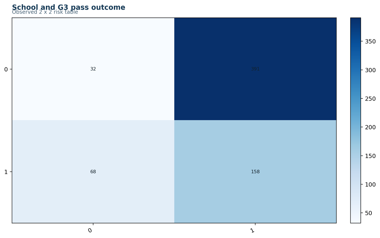
GP has more observations and more passes, while MS has more failures despite its smaller denominator.
MS: 158 pass, 68 fail, N = 226. GP: 391 pass, 32 fail, N = 423.
The event totals alone are insufficient; each pass count must be divided by its school total.
All reported effect measures can be rebuilt from these four cells.
Python Chart 2: Relative Risk Group Risks
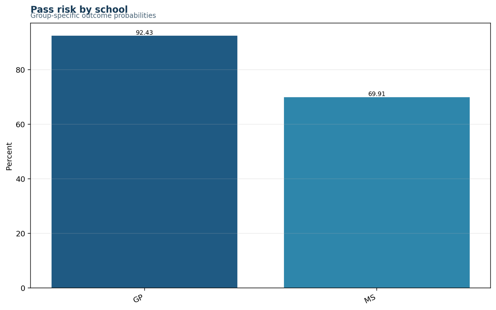
GP has the higher pass risk: 92.43% versus 69.91% in MS.
The vertical difference is 22.52%, or 225.2 passes per 1,000.
Wilson intervals are 63.64%–75.52% for MS and 89.52%–94.59% for GP.
The chart shows the baseline probabilities that give the ratio substantive meaning.
Python Chart 3: Relative Risk Estimate and Confidence Interval
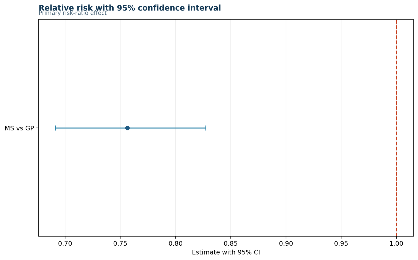
RR = 0.756332.
95% CI = 0.691394 to 0.827368.
The complete interval lies below 1, supporting a lower MS pass probability.
The interval corresponds to a relative shortfall of about 17.26% to 30.86%.
Python Chart 4: Relative Risk Outcome Counts
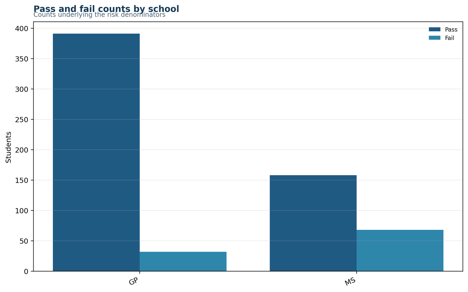
MS has 158 passes and GP has 391.
MS has 68 failures and GP has 32.
GP is larger, so counts cannot be compared without converting them to risks.
MS contributes 68% of all failures while representing only 34.82% of the sample.
Python Chart 5: Relative Risk Result Summary
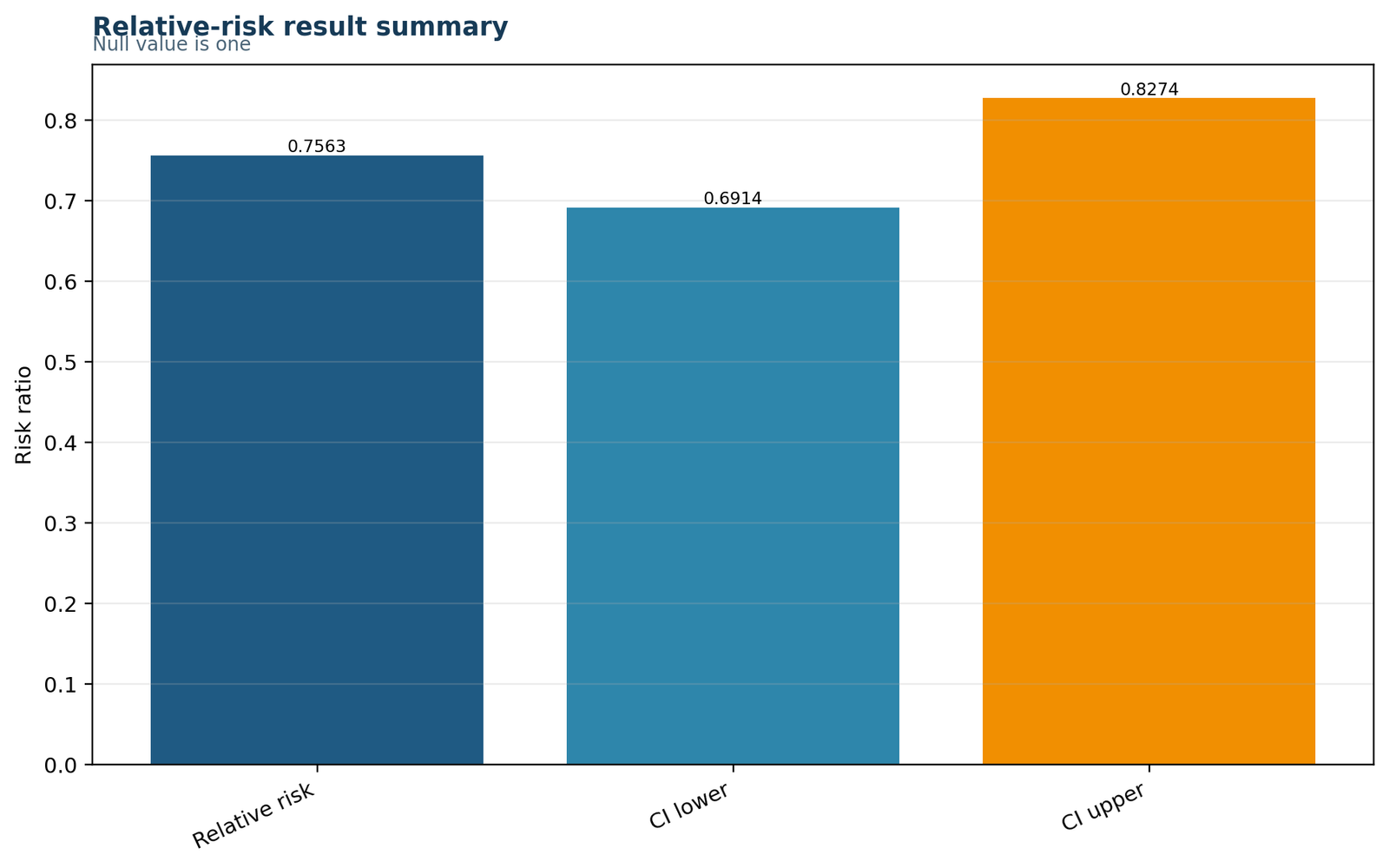
RR = 0.7563, indicating a 24.37% relative shortfall.
RD = -0.2252, indicating a 22.52% absolute shortfall.
Failure RR = 3.9773.
Lead with the event definition, both risks, RR and 95% CI; add RD for practical meaning.
Cross-Chart Data Reconciliation
The five Python figures are different views of one table, not five independent analyses. Chart 1 supplies the four counts. Chart 2 divides them by row totals. Chart 3 divides the resulting risks and adds the interval. Chart 4 returns to the event/non-event counts, and Chart 5 combines the outputs. Any disagreement among figures indicates a plotting or labeling problem rather than a new statistical result.
| Python chart | Primary values that must appear | Null or benchmark |
|---|---|---|
| Observed table | 158, 68, 391, 32 | Row and column totals |
| Group risks | 0.6991 and 0.9243 | Probability range 0–1 |
| RR and CI | 0.7563; 0.6914–0.8274 | RR = 1 |
| Outcome counts | 549 passes; 100 failures | N = 649 |
| Summary | RR, CI, RD and both risks | All values reconcile |
R Relative Risk Charts in Paired Rows
The R section retains the permanent sample’s paired horizontal chart layout. Each pair is followed by separate data explanations so that charts remain compact without losing analytical detail.
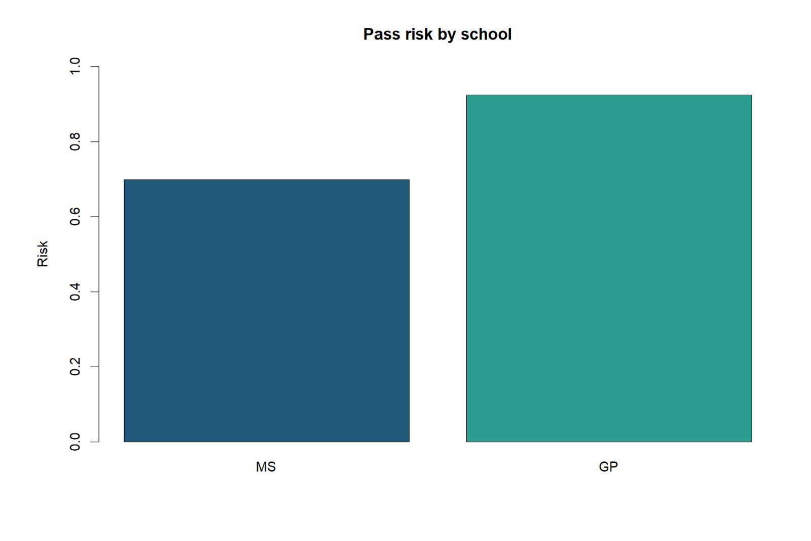
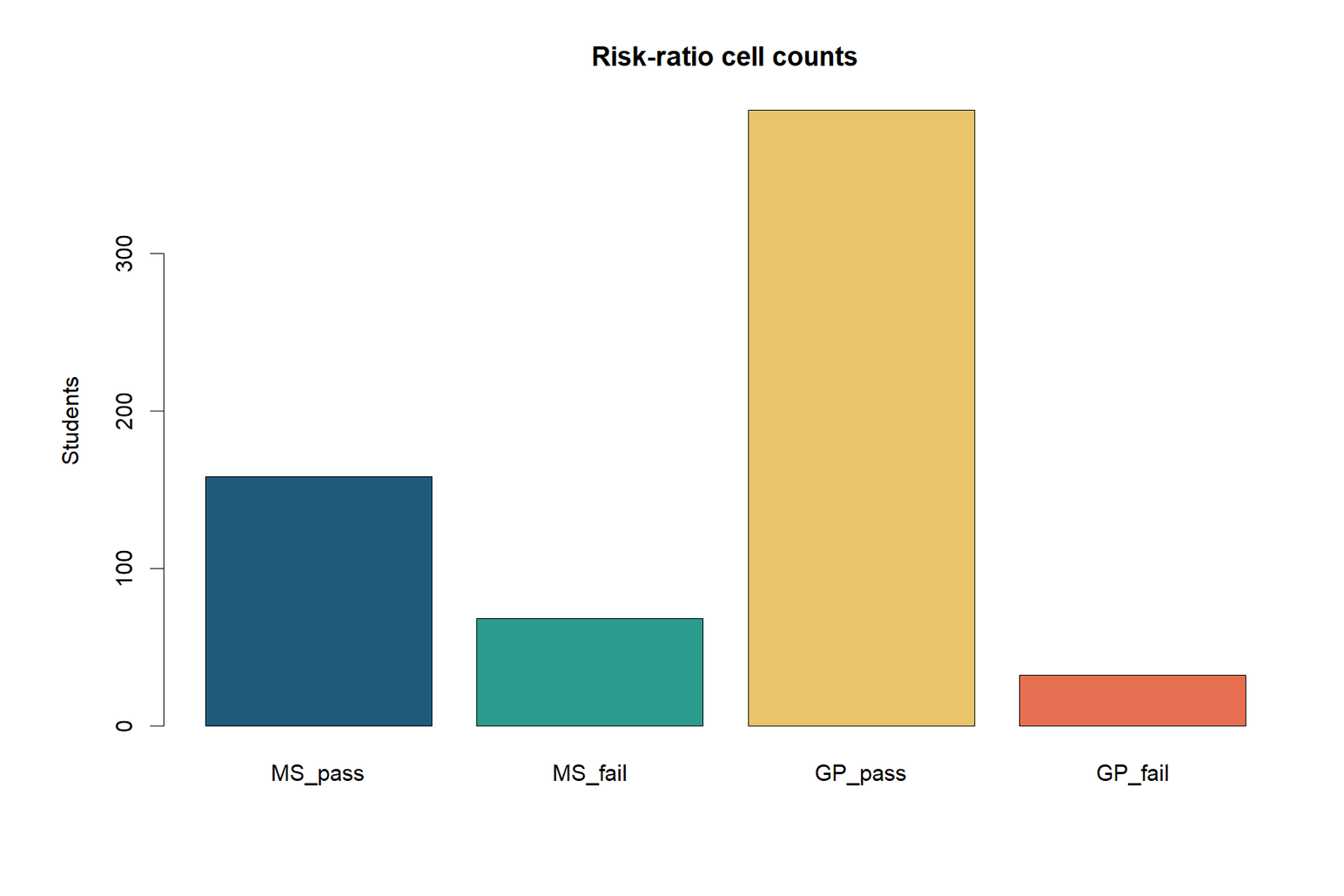
R chart pair 1: Observed 2 × 2 table and School-specific pass risks
Observed 2 × 2 table
The observed table displays 158/68 for MS and 391/32 for GP. The row totals must equal 226 and 423.
School-specific pass risks
The school-risk chart shows 69.91% for MS and 92.43% for GP.
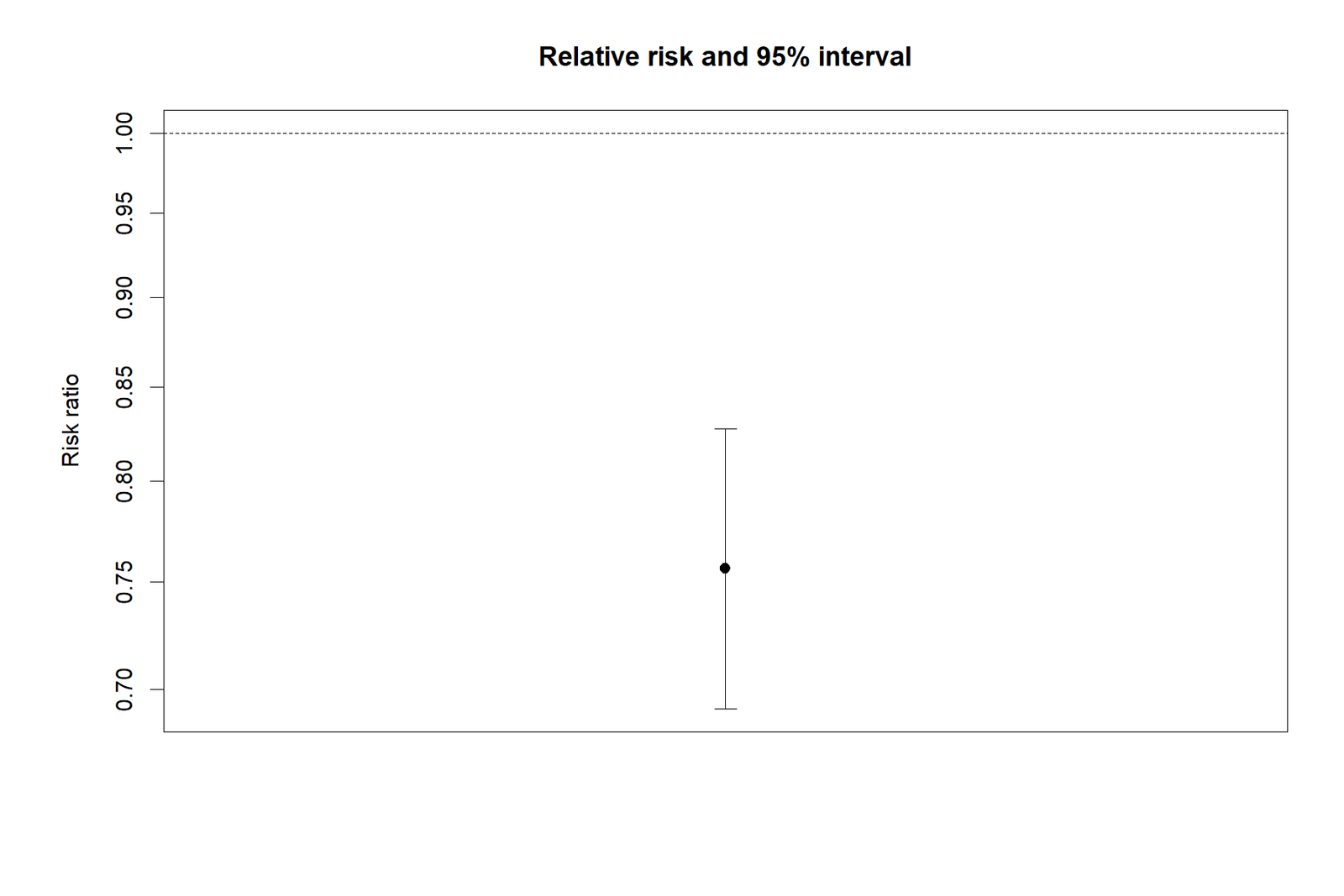
R chart pair 2: Relative risk calculation components and Confidence interval around the risk ratio
Relative risk calculation components
The component chart should show the two risk fractions and their quotient 0.756332.
Confidence interval around the risk ratio
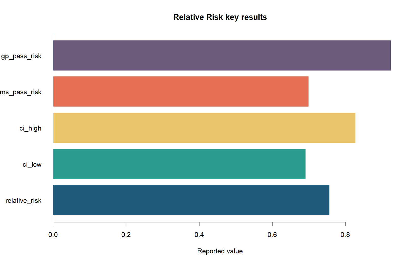
The confidence interval runs from 0.691394 to 0.827368 around RR = 0.756332.
R chart pair 3: Absolute and relative effect measures and R result summary
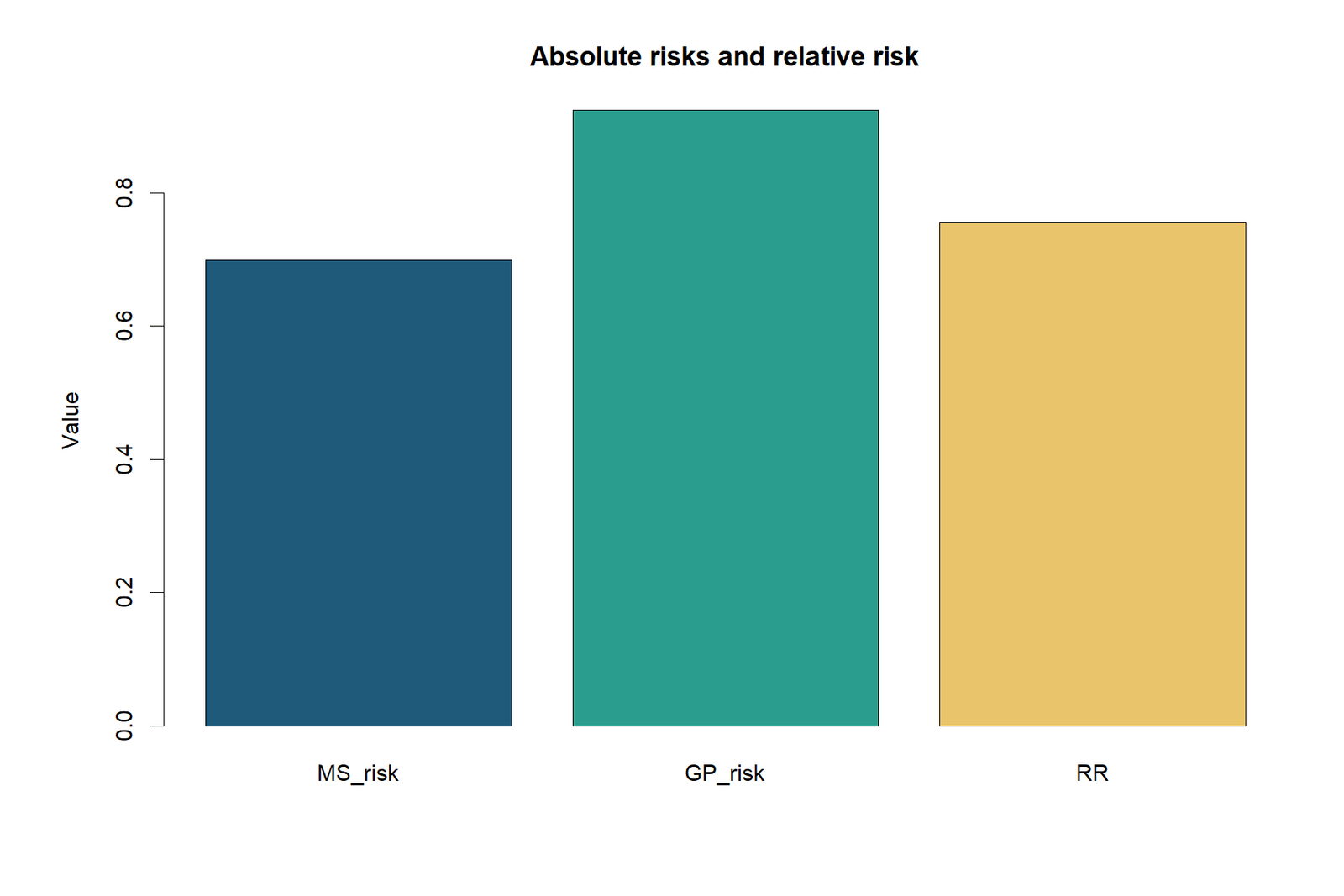
Absolute and relative effect measures
The chart contrasts RR = 0.7563, relative shortfall = 24.37%, and RD = -22.52%.
R result summary
The summary should repeat both group risks, the ratio and its interval without rounding inconsistencies.
Why the R Charts Are Paired
The paired layout keeps the observed table beside the school-risk comparison, the calculation components beside the interval, and the absolute/relative measures beside the final summary. This ordering follows the analysis sequence from counts to probabilities to inference to reporting. On mobile, each chart and explanation collapses to one column while retaining the same order.
R Output Audit
| Audit point | Correct R output | Interpretive consequence |
|---|---|---|
| Matrix row order | MS first, GP second | RR remains below 1. |
| Event column | Pass first | The ratio describes passing. |
| Log SE | 0.045801897 | Produces the reported interval width. |
| Confidence limits | 0.691394 and 0.827368 | Equality value 1 is excluded. |
| Absolute difference | −0.225235 | MS has the lower pass probability. |
Relative Risk in Python, R, SPSS, SAS and Excel
Relative Risk in Python
Build the observed table, calculate each risk explicitly, then apply the Katz interval to the log risk ratio. The code should preserve the MS/GP order.
- MS risk:
158/(158+68) - GP risk:
391/(391+32) - RR:
risk_ms/risk_gp - CI: exponentiate the log limits
Use the categorical data analysis in Python guide for broader table workflows.
Relative Risk in R
Base R is sufficient for transparent arithmetic. Packages can also calculate risk ratios, but the raw counts and group order should be checked before accepting package labels.
- Create
matrix(c(158,68,391,32), byrow=TRUE). - Calculate row risks.
- Calculate the log standard error.
- Exponentiate the 95% limits.
Relative Risk in SPSS
SPSS CROSSTABS can report risk estimates for a 2 × 2 table. The row and column order determine which risk ratio is printed, so verify the reported direction against 69.91% and 92.43%.
- Rows: school
- Columns: pass indicator
- Statistics: RISK and CHISQ
- Cells: count and row percent
Relative Risk in Excel
The fresh workbook separates input data, observed tables, calculations, diagnostics and reporting. Formula cells reproduce RR and the Katz interval without requiring an add-in.
- Risk formulas use row totals.
- The ratio divides MS by GP.
- The CI uses
LN,EXPandSQRT. - The Reporting sheet reconciles workbook and verified values.
Relative Risk in SAS
PROC FREQ can produce risk estimates from the 2 × 2 table. Use ORDER=DATA or explicit formats so the first row and event column match the intended comparison.
- Enter the four counts with a frequency variable.
- Use
TABLES school*pass / RELRISK. - Apply
WEIGHT count. - Check the printed reference direction.
Cross-Software Reconciliation
Independent software should agree to rounding. A difference usually indicates reversed groups, reversed event coding, a continuity correction, or a different confidence-interval method.
- RR = 0.756331621
- SE ln(RR) = 0.045801897
- Lower = 0.691394010
- Upper = 0.827368349
Software Agreement Table
| Platform | Primary calculation | Expected RR | Expected 95% CI | Direction audit |
|---|---|---|---|---|
| Python | Direct formula | 0.756332 | 0.691394–0.827368 | MS / GP |
| R | Direct formula | 0.756332 | 0.691394–0.827368 | MS / GP |
| SPSS | CROSSTABS risk estimate | 0.756332 | Approximately 0.691394–0.827368 | Check row/event order |
| SAS | PROC FREQ RELRISK | 0.756332 | Approximately 0.691394–0.827368 | Check ORDER=DATA |
| Excel | Formula workbook | 0.756332 | 0.691394–0.827368 | MS / GP |
Rounding and Method Differences
Software may display 0.76, 0.756 or 0.756332 depending on output settings. Such rounding is harmless when the underlying calculation agrees. Confidence intervals can differ slightly if a program uses exact, score, bootstrap or continuity-corrected methods instead of the Katz log interval. The method name should therefore accompany the limits when outputs are compared.
Minimum Reproducibility Record
| Item | Value to preserve | Reason |
|---|---|---|
| Group order | MS / GP | Controls ratio direction. |
| Event coding | G3 ≥ 10 | Controls which probability is compared. |
| Counts | 158, 68, 391, 32 | Allows full reconstruction. |
| CI method | Katz log interval | Explains the reported limits. |
| Confidence level | 95% | Determines the critical value. |
| Rounding | Retain at least six decimals internally | Prevents cross-file discrepancies. |
Expandable Relative Risk Code
Python code
import math

a, b, c, d = 158, 68, 391, 32
risk_ms = a / (a + b)
risk_gp = c / (c + d)
rr = risk_ms / risk_gp
se_log = math.sqrt(1/a - 1/(a+b) + 1/c - 1/(c+d))
low = math.exp(math.log(rr) - 1.9599639845 * se_log)
high = math.exp(math.log(rr) + 1.9599639845 * se_log)
risk_difference = risk_ms - risk_gp
print(risk_ms, risk_gp, rr, low, high, risk_difference)
Expected RR: 0.756331621; expected CI: 0.691394010 to 0.827368349.
R code
a <- 158; b <- 68; c <- 391; d <- 32
risk_ms <- a / (a + b)
risk_gp <- c / (c + d)
rr <- risk_ms / risk_gp
se_log <- sqrt(1/a - 1/(a+b) + 1/c - 1/(c+d))
ci <- exp(log(rr) + c(-1, 1) * qnorm(.975) * se_log)
rd <- risk_ms - risk_gp
c(risk_ms=risk_ms, risk_gp=risk_gp, rr=rr, lower=ci[1], upper=ci[2], rd=rd)
SPSS syntax
DATA LIST LIST / school (A2) pass count.
BEGIN DATA
MS 1 158
MS 0 68
GP 1 391
GP 0 32
END DATA.
WEIGHT BY count.
CROSSTABS
 /TABLES=school BY pass
 /FORMAT=AVALUE TABLES
 /STATISTICS=RISK CHISQ
 /CELLS=COUNT ROW EXPECTED.
WEIGHT OFF.
Confirm that the risk estimate corresponds to MS divided by GP for pass = 1.
SAS code
data rr_counts;
  input school $ pass count;
  datalines;
MS 1 158
MS 0 68
GP 1 391
GP 0 32
;
run;
proc freq data=rr_counts order=data;
  tables school*pass / relrisk chisq;
  weight count;
run;
Excel formulas
MS risk: =B5/(B5+C5)
GP risk: =B6/(B6+C6)
Relative risk: =B11/B12
SE ln(RR): =SQRT(1/B5-1/(B5+B6)+1/B7-1/(B7+B8))
Lower 95% CI: =EXP(LN(B13)-1.9599639845*B14)
Upper 95% CI: =EXP(LN(B13)+1.9599639845*B14)
Risk difference: =B11-B12How to Interpret and Report Relative Risk
Interpretation Sequence
| Reporting step | Current data statement |
|---|---|
| Define the event | Pass means G3 ≥ 10. |
| Name the groups | MS is compared with GP. |
| Report both risks | MS = 69.91%; GP = 92.43%. |
| Report the ratio | RR = 0.76. |
| Report precision | 95% CI [0.69, 0.83]. |
| Add absolute meaning | Risk difference = -22.52%. |
| State the design limit | The comparison is observational and unadjusted. |
APA-Style Worked Report
A relative risk analysis compared the probability of achieving G3 ≥ 10 in MS with the probability in GP. The pass risk was 69.91% in MS (158/226) and 92.43% in GP (391/423). The estimated risk ratio was RR = 0.76, 95% CI [0.69, 0.83], indicating that the observed MS pass probability was approximately 75.63% of the GP pass probability. The absolute risk difference was -22.52%, equivalent to about 225 fewer passes per 1,000 students in MS. Because school membership was not randomized, the result should be interpreted as an unadjusted association rather than a causal effect.
Data Discussion
Relative Scale
The point estimate of 0.7563 corresponds to a 24.37% lower pass probability in MS relative to GP. The 95% interval supports a relative shortfall between 17.26% and 30.86%.
Absolute Scale
The pass probabilities differ by 22.52%. This is a large practical separation: approximately 225.2 students per 1,000 on the observed scale.
Complementary Outcome
The failure risk is 30.09% in MS and 7.57% in GP, producing a failure RR of 3.98. This strengthens the directional interpretation but should not replace the prespecified pass analysis.
Underlying Grades
MS has mean G3 = 10.65 and median 11, while GP has mean G3 = 12.58 and median 13. The binary result is consistent with the continuous grade pattern.
Reusable Reporting Templates
Always include the event definition and group direction.
Significant Two-Sided Result
Interval excludes 1
A relative risk analysis compared event risk in Group 1 with Group 2.
Risk was risk 1 versus risk 2, RR = estimate, 95% CI [lower, upper].
The interval excluded 1, supporting a difference in event probability.
Non-Significant Result
Interval includes 1
RR = estimate, 95% CI [lower, upper].
The interval included 1, so the data did not establish a difference in risk at the selected confidence level.
Directional or One-Sided Claim
Prespecify
State the directional hypothesis and reference group before examining the data.
Do not convert a two-sided result into a one-sided claim after observing RR < 1.
Result Table for a Report or Dissertation
| Comparison | Events / total | Risk | Relative risk | 95% CI | Risk difference |
|---|---|---|---|---|---|
| MS versus GP: G3 ≥ 10 | 158/226 versus 391/423 | 0.6991 versus 0.9243 | 0.7563 | 0.6914–0.8274 | −0.2252 |
A compact table should not replace the written interpretation. The text must still name the event, direction and observational design. Conversely, a narrative without the raw counts prevents readers from checking the calculation.
Discussion Paragraph Focused on the Data
The difference is not driven merely by GP’s larger sample. After division by each school’s denominator, GP retains a 92.43% pass risk compared with 69.91% in MS. The ratio estimate places MS at 75.63% of the GP probability, and the confidence interval restricts the plausible ratio to 69.14%–82.74%. On the absolute scale, the 22.52-point gap corresponds to roughly 50.5 fewer observed MS passes than would be expected if the MS group had the GP pass rate. The raw G3 summaries—mean 10.65 in MS versus 12.58 in GP—support the same direction. Nevertheless, the unadjusted school comparison cannot separate school context from differences in student composition.
What Not to Write
Common Relative Risk Mistakes and Corrections
| Mistake | Incorrect consequence | Correction using the current data |
|---|---|---|
| Dividing event counts | 158/391 = 0.404 is not RR | Divide 158/226 by 391/423. |
| Reversing the reference | Reports 1.322 instead of 0.756 | State MS/GP before calculation. |
| Switching the event | Reports failure RR without notice | State G3 ≥ 10 as the event. |
| Calling odds ratio relative risk | Uses OR = 0.190 as though it were RR | Report OR and RR with their correct names. |
| Ignoring the confidence interval | Treats the point estimate as exact | Report 0.691–0.827. |
| Using total N as denominator | Distorts both group risks | Use 226 for MS and 423 for GP. |
| Claiming causation | Attributes the school difference to school alone | Describe an observational, unadjusted association. |
| Reporting only relative change | Hides baseline probabilities | Add 69.91%, 92.43% and RD = -22.52%. |
| Calling 1/RR an error | Rejects a valid reciprocal | Explain that reciprocal direction answers GP/MS instead. |
| Using NNT causally | Treats 1/|RD| = {1/abs(rd):.2f} as intervention evidence | Do not use NNT/NNH language for this school comparison. |
Why These Errors Survive Superficial Checks
Several incorrect calculations produce plausible-looking positive numbers. The reciprocal 1.3222, failure RR 3.9773 and odds ratio 0.1902 are all mathematically valid for different questions. A generic “does the number look reasonable?” check will not detect the problem. Only explicit labels for group order, event coding and measure type can do so.
Formatting is also part of error prevention. Bordered observed tables, separate risk cards and a clearly marked null value make denominator and direction mistakes easier to see. This is why the post keeps counts, probabilities, ratios and interpretation in distinct boxes rather than merging them into one paragraph.
Relative Risk Practice Questions
1. Calculate the MS pass risk.
Use 158 passes and 68 failures.
2. Calculate the GP pass risk.
Use 391 passes and 32 failures.
3. Calculate and interpret relative risk.
4. Interpret the 95% confidence interval.
5. Express the result on the absolute scale.
6. Recode failure as the event.
7. Explain why OR and RR differ.
8. Identify the causal limitation.
9. Calculate the descriptive MS pass shortfall at the GP risk.
10. Which group contributes most to log-RR uncertainty?
11. Interpret the lower confidence limit.
12. Why does threshold sensitivity not authorize choosing a new cut point?
Relative Risk Reports and Worked Files
Each file uses the same MS-versus-GP direction and the G3 ≥ 10 event definition. Download labels are explicit so the public post does not confuse statistical outputs with chart images.
R PDF ReportR calculations and six result figures.
SPSS PDF OutputCrosstabs, risk estimates and association output.
Worked Excel AnalysisData input, observed table, formula calculations, diagnostics and reporting audit.
How to Use the Four Files Together
Use the Excel workbook to audit raw records and formulas, the Python and R reports to verify independent implementations and figures, and the SPSS output to confirm the standard crosstab risk estimate. Agreement across files is meaningful only when all of them use MS/GP and pass = G3 ≥ 10.
Relative Risk Frequently Asked Questions
What is the relative risk in this example?
The MS-versus-GP pass relative risk is 0.756332. It is calculated from 69.91% divided by 92.43%.
What does RR = 0.756 mean?
The MS pass probability is 75.63% of the GP pass probability, or 24.37% lower on the relative scale.
Is relative risk the same as risk ratio?
Yes. Relative risk and risk ratio are two names for the same ratio of event probabilities.
Why is the null value 1?
A ratio of 1 means the two group risks are equal. Values below or above 1 indicate lower or higher risk in the numerator group.
Why is zero not the null value?
Zero is the null value for a difference, not a ratio. Relative risk is compared with 1.
Does the confidence interval show statistical significance?
Yes. The 95% interval 0.6914 to 0.8274 excludes 1. The interval also shows the plausible magnitude, not only a yes/no decision.
What is the risk difference?
The MS minus GP risk difference is -0.225235, which equals a 22.52% lower absolute pass probability in MS.
Why is the odds ratio different?
The odds ratio is 0.1902. Because passing is common, the odds ratio lies farther from 1 than the relative risk.
What happens if GP is divided by MS?
The reciprocal is 1.3222. It says GP has about 1.32 times the pass probability of MS.
What happens if failure is the event?
The failure-risk ratio is 3.9773, with MS having the higher failure probability.
Can this result prove that school causes the difference?
No. School was not randomized, and the unadjusted comparison may reflect student composition or other confounders.
Can relative risk be calculated in a case-control study?
Usually not directly, because case-control sampling fixes case and control counts rather than preserving population risks. Odds ratios are typically used.
What should be reported with relative risk?
Report event definition, group order, both risks, RR, 95% CI, raw counts and preferably an absolute measure such as risk difference.
Why inspect the raw G3 distribution?
The numeric grades show that the binary result is not isolated: MS mean G3 is 10.65, compared with 12.58 in GP.
Are there any zero-cell problems here?
No. All four cells are positive, so the standard log confidence interval is defined without adding a continuity correction.
Which software result should be trusted?
Trust the result that reconciles to the observed counts and direction. Python, R, SPSS, SAS and Excel should reproduce RR = 0.756332 to rounding.
How much of the confidence-interval variance comes from MS?
Approximately 90.78% of the Katz log variance comes from the MS component, reflecting its smaller sample and event count.
Does the raw numeric G3 outcome tell the same story?
Yes. Mean G3 is 10.65 in MS and 12.58 in GP, while the medians are 11 and 13. The binary pass comparison is consistent with these summaries.
What is the implied absolute gap at the confidence limits?
Using the GP baseline, the RR limits imply MS risks of about 63.91% to 76.48%, compared with the observed GP risk of 92.43%.
Why not report only the reciprocal 1.32?
The reciprocal is valid but reverses the comparison. This post prespecifies MS divided by GP, so 0.7563 is the primary estimate and 1.3222 is only a translated statement.
Relative Risk Conclusion
The complete data analysis begins with 158 passes and 68 failures in MS and 391 passes and 32 failures in GP. These counts produce pass risks of 69.91% and 92.43%, respectively. The MS-versus-GP relative risk is 0.756332, with a 95% confidence interval from 0.691394 to 0.827368.
The result is substantial on both scales: a 24.37% relative shortfall and a 22.52% absolute shortfall in pass probability for MS. The complementary failure-risk ratio of 3.98 and the underlying G3 summaries point in the same direction. The analysis is statistically precise, but it remains an observational, unadjusted school comparison.
The structured tables and charts also show why the result is credible as a description of these records. Every total reconciles, all cells are positive, the group-risk intervals are separated, and threshold sensitivity from G3 ≥ 8 through G3 ≥ 14 preserves RR below 1. These checks strengthen the data interpretation while leaving the causal limitation unchanged.

