
Mantel Haenszel Test: Formula, Calculator, Interpretation, Python, R, SPSS and Excel Guide
Mantel Haenszel Test is the classic stratified method for combining several 2 × 2 tables into one adjusted association test and a common odds-ratio estimate. This guide explains the hypotheses, formulas, interpretation, calculator logic, Python, R, SPSS and Excel workflows, APA reporting, chart-based explanation and downloads through a worked analysis of the association between sex and final-pass status adjusted for study-time strata.
649 observations
MH χ² = 0.9333
Common OR = 0.7999
Mantel Haenszel Test Model Overview
Mantel Haenszel Test is used when the same 2 × 2 association is observed repeatedly across several strata and the analyst wants a single adjusted test and a pooled effect estimate. Instead of collapsing everything into one table and ignoring the stratifying variable, the method respects the stratum structure and asks whether there is a common association after controlling for the stratification factor.
What question does the Mantel Haenszel Test answer?
In this worked example, the research question is whether the association between sex and G3 pass remains after adjusting for studytime. Each study-time level forms a separate 2 × 2 table, and the Mantel Haenszel procedure combines them into a common adjusted result.
What does the common odds ratio mean?
The Mantel Haenszel common odds ratio summarizes the adjusted odds association across strata. A value of 1 indicates no association after adjustment, a value below 1 indicates lower adjusted odds in the numerator group, and a value above 1 indicates higher adjusted odds. In the current workbook, the male-versus-female adjusted common odds ratio is 0.7999.
Worked example at a glance
The four study-time strata contain separate male/female by pass/fail tables. The verified Mantel Haenszel statistic is 0.9333 with p = 0.3340. The common odds ratio is 0.7999 with a 95% confidence interval of 0.5102 to 1.2542. Because the interval includes 1 and the p-value is well above .05, the adjusted association is not statistically significant.
Quick Answer: Mantel Haenszel Test Result
The Mantel Haenszel Test combines four study-time-specific 2 × 2 tables to estimate one adjusted association between sex and pass status. The common-effect estimate is below 1, but the evidence is not statistically significant.
Test summary
- Procedure: Mantel Haenszel common odds-ratio test
- Strata: studytime = 1, 2, 3, 4
- Statistic: MH χ² = 0.9332565
- P-value: 0.3340182
- Adjusted effect: common OR = 0.7999116
- 95% CI: 0.5101770 to 1.2541894
Substantive meaning
- The adjusted male odds of passing are estimated to be about 20% lower than the female odds.
- The confidence interval includes 1, so that reduction is not precise enough to declare a clear adjusted effect.
- The study-time strata do not all have identical raw patterns, but the common-effect summary remains near no effect.
- The overall adjusted evidence is weak rather than decisive.
Table of Contents
- Research question, hypotheses and data design
- When to use the Mantel Haenszel Test
- Mantel Haenszel Test formula and calculation
- Variables and data dictionary
- Stratum tables and complete results
- Mantel Haenszel versus chi-square and crude analysis
- Mantel Haenszel Test calculator workflow
- Python and R chart interpretations
- Python, R, SPSS and Excel workflows
- Expandable software code
- Assumptions, limitations and advanced interpretation
- APA reporting for the Mantel Haenszel Test
- Common mistakes and how to correct them
- Reports and worked Excel download
- Related Salar Cafe guides
- Frequently asked questions
- Conclusion
Research Question, Hypotheses and Data Design
sex with male and female categories.G3 pass coded as pass (G3 ≥ 10) versus fail (G3 < 10).studytime with four levels used to control the association.Research question
Is there an association between sex and final-pass status after adjusting for differences in study-time strata?
Null and alternative hypotheses
| Hypothesis | Statistical statement | Meaning |
|---|---|---|
| Null hypothesis | H0: θMH = 1 | The common adjusted odds ratio across strata equals one. |
| Alternative hypothesis | H1: θMH ≠ 1 | There is a non-null adjusted association after controlling for study time. |
Why this is a stratified analysis
Each study-time level creates its own 2 × 2 table. A simple chi-square test of independence on the collapsed table would ignore possible confounding by study time. The Mantel Haenszel Test preserves the stratum structure and produces an adjusted estimate.
Current data design
The workbook contains 649 students. The observed strata are studytime 1, 2, 3 and 4. Within each stratum, the table is ordered as male pass a, male fail b, female pass c and female fail d. That orientation matters because it determines the direction of the odds ratio.
When to Use the Mantel Haenszel Test
Use the Mantel Haenszel Test when
- You have several 2 × 2 tables representing the same exposure-outcome relationship across strata.
- You want an adjusted association after controlling for one categorical confounder.
- The outcome and exposure are both binary within each stratum.
- A common odds-ratio summary is scientifically meaningful.
- You want a transparent stratified alternative to a regression model.
Choose another method when
- The strata-specific effects differ strongly and no common effect is appropriate.
- You need to control for several covariates simultaneously.
- The outcome is continuous rather than binary.
- The table is not 2 × 2 within each stratum.
- You need model-based estimation with interactions or adjusted predictions.
Simple selection logic
If yes, a stratified method may be suitable.
If yes, the Mantel Haenszel Test is often a good first adjusted analysis.
If yes, combine the strata; otherwise examine heterogeneity or use a regression model.
Useful companion topics are chi-square test, chi-square test of homogeneity, Cramér’s V and logistic regression.
Mantel Haenszel Test Formula and Calculation
The Mantel Haenszel procedure uses each stratum's observed cell count and expected count under the null, then combines them into one chi-square statistic. The common odds ratio is computed from weighted cross-products.
ight]^2}{\sum_h Var(a_h)}
Step 1: List the 2 × 2 tables
| Stratum | a = M pass | b = M fail | c = F pass | d = F fail | n |
|---|---|---|---|---|---|
| 1 | 91 | 32 | 71 | 18 | 212 |
| 2 | 92 | 15 | 172 | 26 | 305 |
| 3 | 21 | 1 | 69 | 6 | 97 |
| 4 | 12 | 2 | 21 | 0 | 35 |
Step 2: Compute stratum expectations and variances
| Stratum | E(a) | Var(a) | a − E(a) |
|---|---|---|---|
| 1 | 93.9906 | 9.3503 | −2.9906 |
| 2 | 92.6164 | 8.1089 | −0.6164 |
| 3 | 20.4124 | 1.1508 | 0.5876 |
| 4 | 13.2000 | 0.4659 | −1.2000 |
Step 3: Combine the deviations
The sum of the deviations is −4.2193 and the sum of the variances is 19.0760. Substituting into the formula gives the verified Mantel Haenszel chi-square:
Step 4: Obtain the p-value
The Mantel Haenszel statistic is compared with a chi-square distribution with 1 degree of freedom. The verified p-value is 0.3340182, which is not statistically significant at α = .05.
Step 5: Compute the common odds ratio
Using the weighted cross-product formula, the common odds ratio is:
The 95% confidence interval is 0.5101770 to 1.2541894. Because the interval includes 1, the adjusted common effect is not statistically distinguishable from no association.
Variables and Data Dictionary
| Variable | Role | Coding | Use in the analysis |
|---|---|---|---|
| sex | Exposure | M = male, F = female | The binary grouping variable whose adjusted association with pass is tested. |
| G3 | Original outcome source | Final grade from 0 to 19 | Used to derive pass/fail status. |
| G3 pass | Binary outcome | 1 = G3 ≥ 10, 0 = G3 < 10 | The event variable inside each 2 × 2 table. |
| studytime | Stratifier | 1, 2, 3, 4 | Controls the association by creating the four strata. |
Stratum-specific pass rates
| Stratum | Male pass rate | Female pass rate | Stratum OR |
|---|---|---|---|
| 1 | 0.7398 | 0.7978 | 0.7210 |
| 2 | 0.8598 | 0.8687 | 0.9271 |
| 3 | 0.9545 | 0.9200 | 1.8261 |
| 4 | 0.8571 | 1.0000 | 0.0000 |
The raw strata show some variation. In strata 1, 2 and 4 the male odds are lower, whereas stratum 3 shows a male odds ratio above 1. This is exactly why a common-effect procedure should be accompanied by a heterogeneity check such as the Breslow Day Test.
Worked Stratified 2 × 2 Tables and Complete Results
Separate 2 × 2 tables combined in one adjusted analysis
Common-effect chi-square with 1 degree of freedom
Fails to reject the null at α = .05
Adjusted male-versus-female pass odds
Includes the null value of 1
Unstratified association before adjustment
| Metric | Value | Interpretation |
|---|---|---|
| Mantel Haenszel statistic | 0.9332564901 | The combined adjusted chi-square evidence is small. |
| P-value | 0.3340181554 | No statistically significant adjusted association. |
| Common odds ratio | 0.7999116499 | Adjusted male pass odds are estimated to be about 0.80 of female pass odds. |
| 95% CI lower | 0.5101770460 | Compatible with a moderate reduction in odds. |
| 95% CI upper | 1.2541894087 | Also compatible with little or no difference and even a mild increase. |
Crude versus adjusted story
The unstratified male-versus-female odds ratio from the collapsed table is 0.6486, whereas the adjusted Mantel Haenszel common odds ratio is 0.7999. The move toward 1 after adjustment suggests that study time explains part of the crude association. That is exactly the kind of confounding pattern for which a stratified adjusted analysis is useful.
Mantel Haenszel Test Versus Crude Chi-Square and Logistic Regression
| Method | What it uses | Key output | Interpretive role |
|---|---|---|---|
| Crude 2 × 2 analysis | One collapsed table | Crude OR = 0.6486 | Shows the unadjusted association without controlling for study time. |
| Mantel Haenszel Test | Four stratified 2 × 2 tables | MH χ² = 0.9333, OR = 0.7999 | Provides an adjusted common association across study-time strata. |
| Chi-square test of independence | One contingency table | Unadjusted association test | Useful for raw association but not sufficient when a stratifier matters. |
| Logistic regression | Model-based adjustment | Adjusted coefficients and interactions | More flexible when multiple controls or interactions are needed. |
The Mantel Haenszel Test sits between a simple chi-square analysis and a full regression model. It is more informative than a crude association because it controls one categorical confounder, but it is simpler and more transparent than a multivariable model.
Mantel Haenszel Test Calculator: Step-by-Step Workflow
A correct Mantel Haenszel Test calculator should accept multiple 2 × 2 tables, compute the expected counts and variances within each stratum, return the MH statistic, and report the common odds ratio with a confidence interval.
Calculator inputs for the worked example
| Input | Value | Meaning |
|---|---|---|
| Number of strata | 4 | Studytime levels 1 through 4. |
| Table orientation | M pass, M fail, F pass, F fail | Determines the direction of the odds ratio. |
| Stratum counts | (91,32,71,18), (92,15,172,26), (21,1,69,6), (12,2,21,0) | The four 2 × 2 tables. |
| Alpha level | 0.05 | Decision threshold. |
Calculator steps
- Enter each 2 × 2 table separately rather than collapsing them.
- Keep the same cell orientation in every stratum.
- Review the stratum-specific odds ratios before trusting the common odds ratio.
- Read the common OR and its confidence interval together with the p-value.
- If heterogeneity appears strong, interpret the pooled effect cautiously and consider a separate Breslow Day Test.
Six Python and R Mantel Haenszel Test Chart Interpretations
The Python and R workflows illustrate the same underlying Mantel Haenszel story: how each stratum behaves, how large the stratum tables are, whether the stratum-specific effects look homogeneous, and what the final common-effect result means.
Chart 1: Stratum odds ratios and common effectPython + R
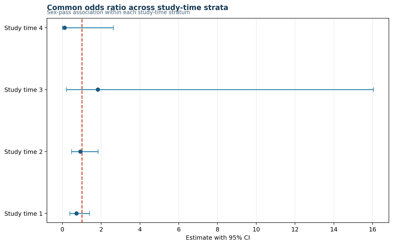
Most strata have odds ratios below 1, but one stratum is above 1 and one has a zero cell that forces the raw stratum OR to 0.
Stratum ORs are 0.7210, 0.9271, 1.8261 and 0.0000. The common OR is 0.7999.
The common-effect summary lies below 1, but the variation across strata reminds us to think about heterogeneity before overinterpreting the pooled result.
This chart is the fastest visual summary of whether a pooled odds ratio is directionally sensible.
Chart 2: Stratum counts and pass totalsPython + R
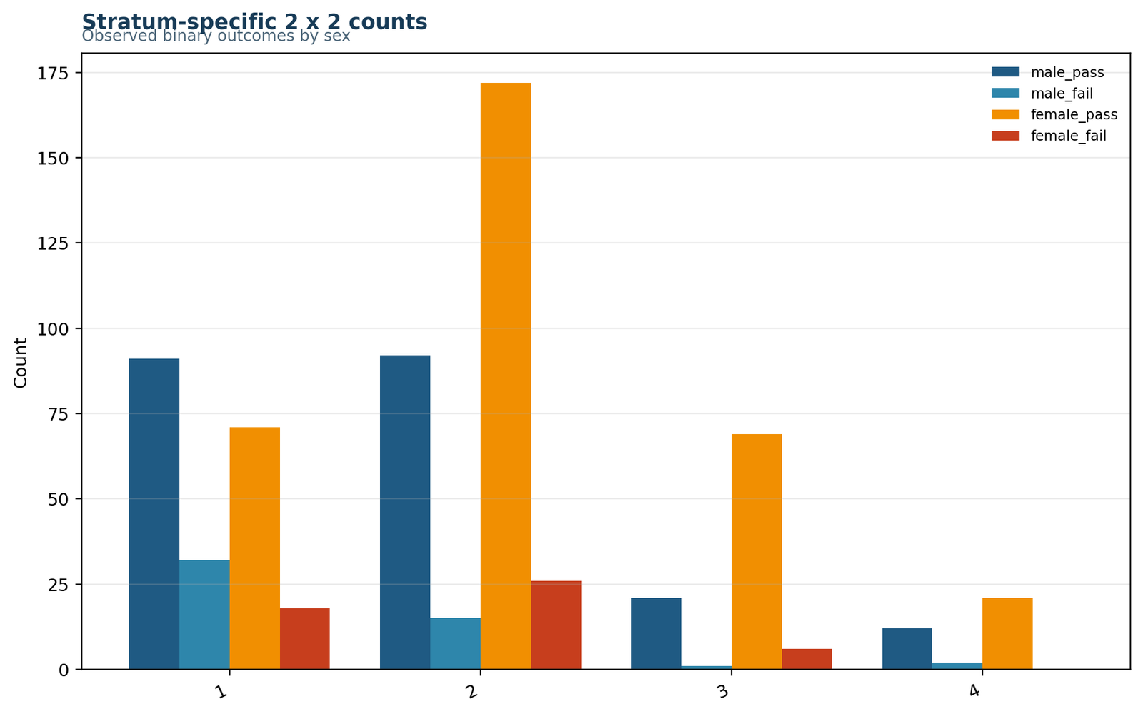
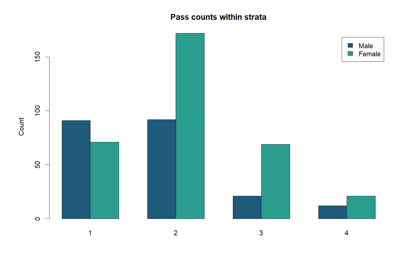
Stratum 2 is the largest and therefore has the strongest influence on the pooled estimate.
Stratum totals are 212, 305, 97 and 35, with the fourth stratum contributing comparatively little information.
The common effect is not a simple average of the stratum ORs; larger, more informative strata receive more weight.
Understanding the stratum sizes helps explain why the common OR ends up near 0.80 rather than being dominated by the extreme small-stratum OR.
Chart 3: Heterogeneity profile and fail countsPython + R
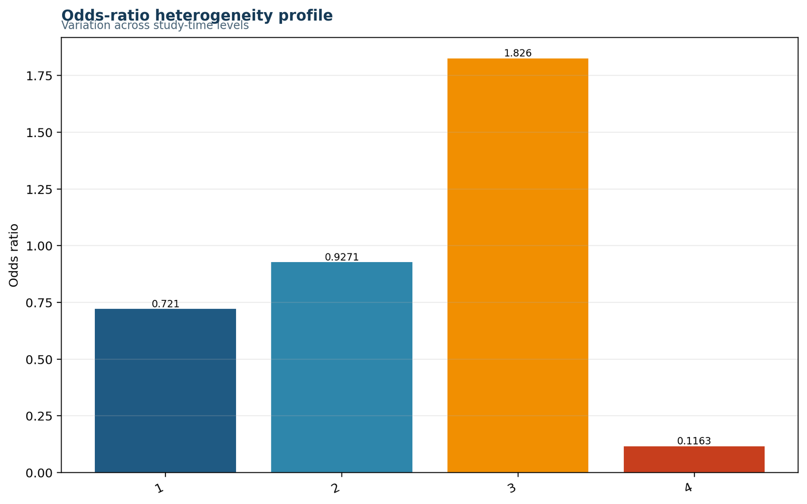
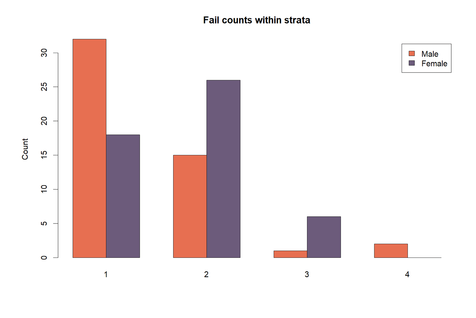
The fourth stratum contains a zero female-fail cell, and the third stratum has very few male failures.
Male fails are 32, 15, 1 and 2; female fails are 18, 26, 6 and 0.
Sparse failure cells can create unstable or extreme raw stratum odds ratios, which is why a pooled adjusted estimate can be more informative than reading each OR in isolation.
This is also why the common-effect assumption should be checked and why continuity decisions matter in small strata.
Chart 4: Absolute log effects and stratum sizesPython + R
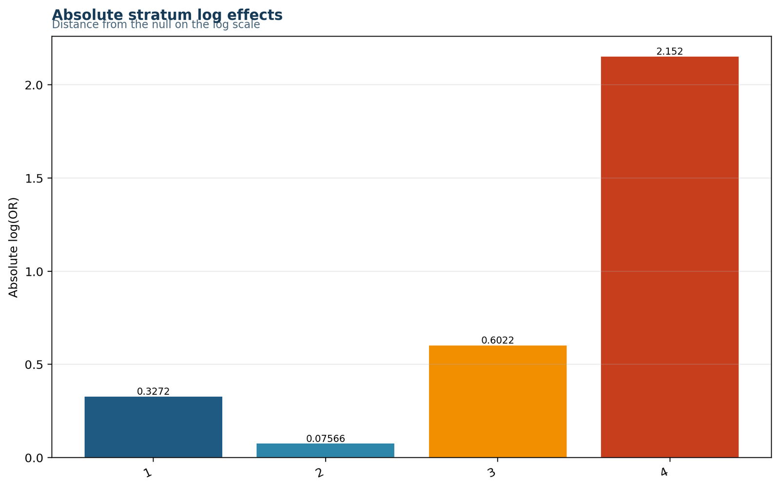
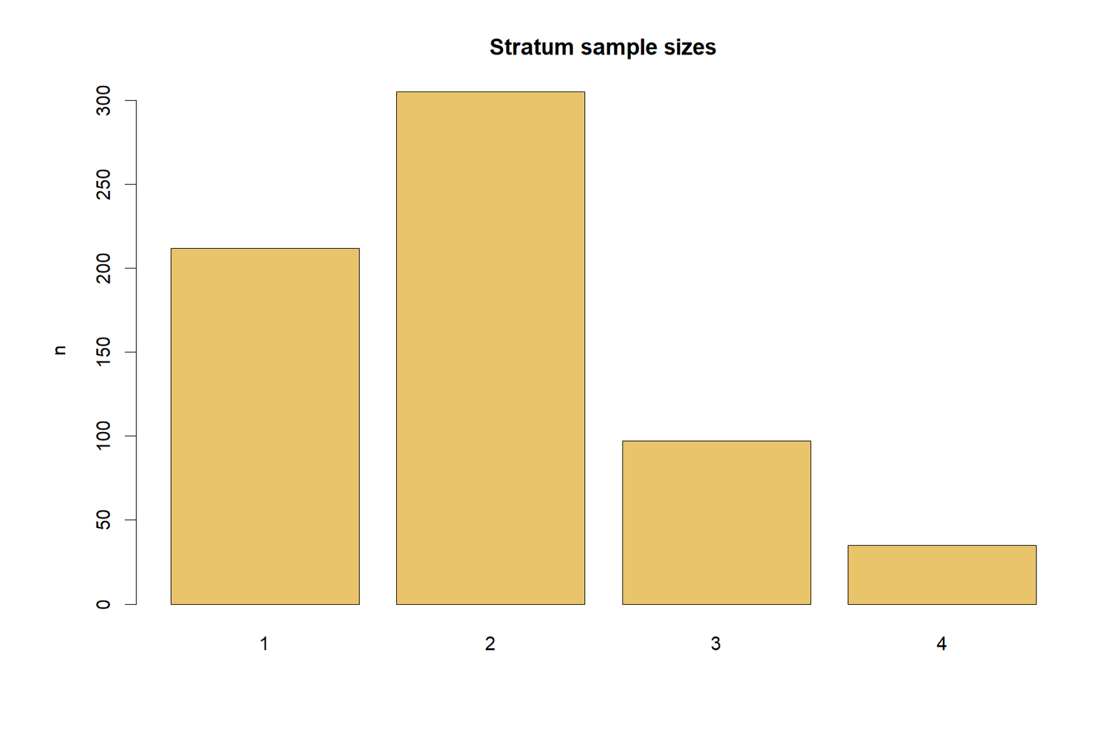
The most extreme apparent effect does not occur in the largest stratum.
Stratum 3 has an OR above 1.8 but only 97 observations, whereas stratum 2 has 305 observations and an OR close to 0.93.
Magnitude alone is not enough; the pooled result balances effect size and information content across strata.
This chart pair explains why the adjusted common OR is moderate and why the significance test is weak.
Chart 5: Log odds ratio by stratum and common-effect intervalPython + R
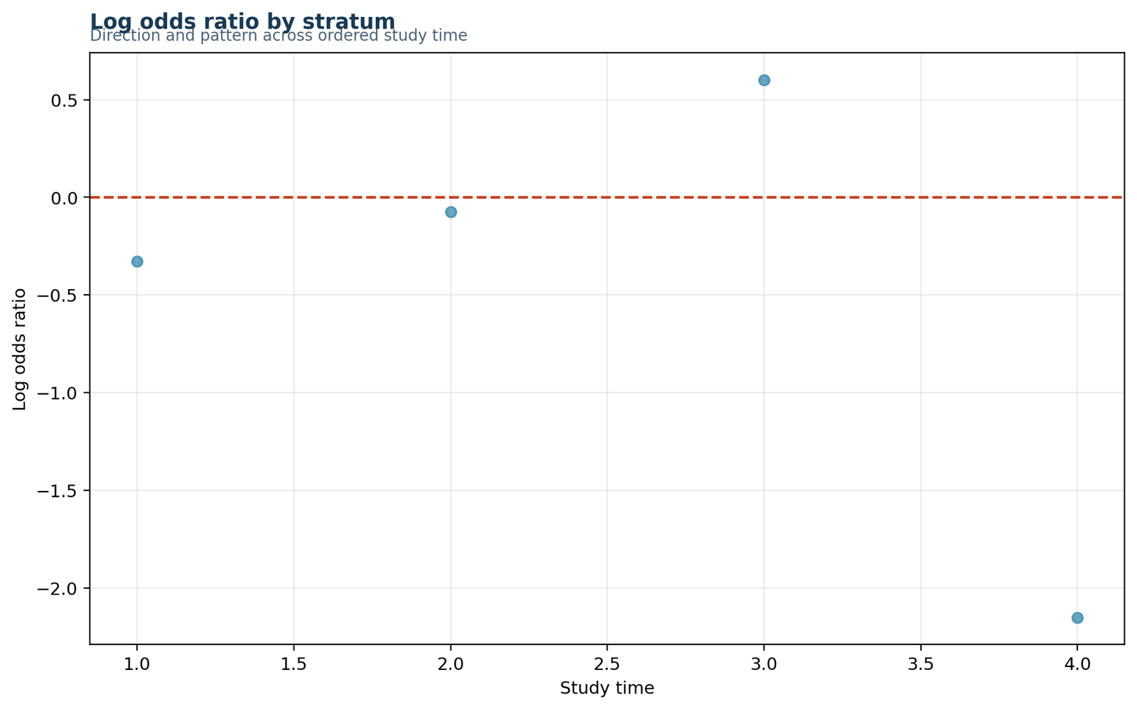
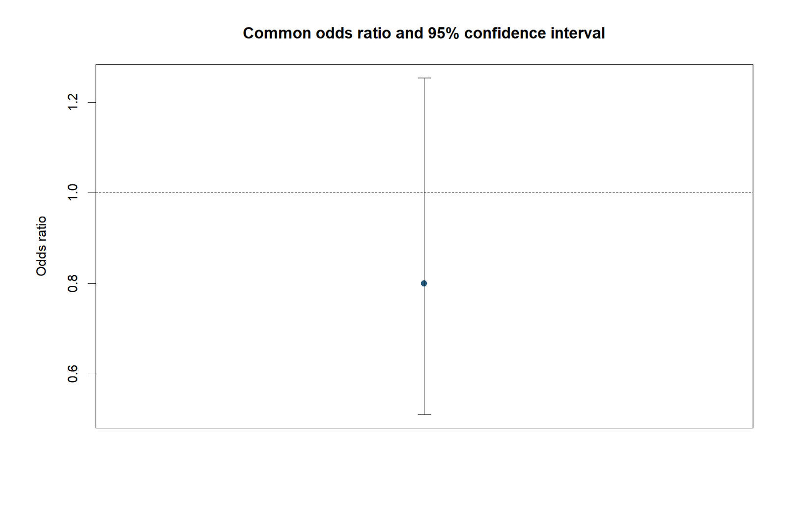
The common-effect interval crosses 1, confirming the non-significant adjusted result.
Common OR = 0.7999 with 95% CI 0.5102 to 1.2542.
The data are compatible with a meaningful reduction in male pass odds, but also compatible with little or no adjusted difference.
The interval communicates uncertainty better than the p-value alone.
Chart 6: Result summaryPython + R
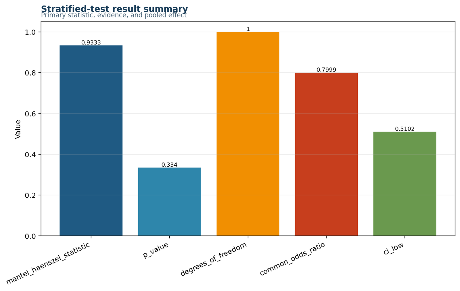
The summary chart condenses the adjusted common-effect analysis into one compact result panel.
MH χ² = 0.9333, p = 0.3340, common OR = 0.7999 and 95% CI 0.5102 to 1.2542.
The adjusted evidence is not statistically significant, and the effect estimate remains uncertain.
This is the best visual for reports, teaching slides and quick communication of the final conclusion.
Mantel Haenszel Test in Python, R, SPSS and Excel
Python workflow
Python is convenient for building the stratum tables, computing the Mantel Haenszel statistic, extracting the common odds ratio and creating the diagnostic charts. For broader background, see categorical data analysis in Python.
- Create one 2 × 2 table for each study-time stratum.
- Keep the same cell ordering in every stratum.
- Compute the MH statistic and common OR.
- Check the confidence interval and heterogeneity context.
- Generate stratum and summary charts.
R workflow
R provides reliable support for stratified 2 × 2 analyses and is well suited to effect-estimate plots and common-effect summaries. See categorical data analysis in R.
- Represent the data as a three-dimensional table.
- Call the Mantel Haenszel procedure for the stratified association.
- Extract the common odds ratio and interval.
- Display stratum-specific and pooled results visually.
- Add a heterogeneity check when relevant.
SPSS workflow
SPSS can produce stratified crosstabs, odds ratios and Mantel Haenszel-type outputs for layered tables. It is also useful for exporting the study-time-specific tables and supporting diagnostics. See categorical data analysis in SPSS.
- Define sex, pass/fail and studytime clearly.
- Use layered crosstabs by studytime.
- Request the Mantel Haenszel statistics and odds ratios.
- Verify the direction of the exposure and outcome coding.
- Export the output PDF and compare it with the verified workbook.
Excel workflow
The Excel workbook used here shows every stage of the computation explicitly: input data, observed tables, calculations, diagnostics and reporting. That makes it useful for teaching and manual verification.
- Enter or import the original row-level data.
- Create the four study-time-specific 2 × 2 tables.
- Calculate E(a), Var(a), a−E(a), ad/n and bc/n.
- Combine the strata into the MH statistic and common OR.
- Reference the verified p-value and confidence interval in the reporting sheet.
Why not just use logistic regression?
Logistic regression is more flexible, but the Mantel Haenszel Test remains valuable when the goal is a transparent one-confounder adjustment with a clear common odds-ratio interpretation. It is often easier to teach, easier to verify by hand and often ideal as a first adjusted analysis before moving to a model-based workflow.
Expandable Code for the Mantel Haenszel Test
Python pseudo-code for the Mantel Haenszel Test
tables = [
    [[91, 32], [71, 18]],
    [[92, 15], [172, 26]],
    [[21, 1], [69, 6]],
    [[12, 2], [21, 0]]
]
# compute stratum-specific values
# combine them into the MH statistic
# compute the common odds ratio and confidence interval
R pseudo-code for the Mantel Haenszel Test
# create a 2 x 2 x 4 array
# run mantelhaen.test(x)
# extract the common odds ratio and confidence interval
# summarize the strata and create plots
Excel formula ideas
E(a) = ((a+b)*(a+c))/n
Var(a) = ((a+b)*(c+d)*(a+c)*(b+d)) / (n^2*(n-1))
MH_stat = (SUM(a_minus_E)^2) / SUM(var_a)
OR_MH = SUM(a*d/n) / SUM(b*c/n)
Assumptions, Limitations and Advanced Interpretation
Assumptions
- Each stratum is a valid 2 × 2 table for the same exposure-outcome question.
- Observations are independent within and across strata.
- The strata are meaningful and correctly defined.
- A common odds ratio is a reasonable summary.
- The coding direction is consistent across all strata.
Limitations
- The method adjusts for only a stratification structure, not multiple continuous covariates.
- Strong effect heterogeneity weakens the meaning of the pooled odds ratio.
- Sparse strata can produce unstable stratum-specific odds ratios.
- The common odds ratio is not as flexible as a full model-based approach.
- Collapsing a quantitative covariate into strata may lose information.
The biggest interpretive safeguard is to separate common-effect estimation from homogeneity checking. The Mantel Haenszel Test can estimate a common adjusted association, but it does not by itself prove that a single common odds ratio describes every stratum equally well. That is why a separate Breslow Day Test is usually recommended.
APA Reporting for the Mantel Haenszel Test
Completed worked-example report
Not significant
A Mantel Haenszel common odds-ratio analysis examined the association between sex and final-pass status while adjusting for four study-time strata.
The adjusted association was not statistically significant, χ2MH(1, N = 649) = 0.93, p = .334.
The common odds ratio was ORMH = 0.80, 95% CI [0.51, 1.25].
After adjustment for study time, male pass odds were estimated to be lower than female pass odds, but the interval included 1 and the evidence was not statistically reliable.
Table direction: male versus female pass odds. Homogeneity should be evaluated separately before emphasizing one common effect.
Reusable APA template
Fill-in template
A Mantel Haenszel analysis was conducted to examine the association between [exposure] and [binary outcome] while adjusting for [stratifying variable].
The common adjusted association was [significant/not significant], χ2MH(1, N = [N]) = [statistic], p = [p].
The common odds ratio was ORMH = [estimate], 95% CI [[lower], [upper]].
This indicates [plain-language adjusted interpretation].
Always identify the numerator group and event coding because reversing either changes the odds-ratio direction.
Common Mantel Haenszel Test Mistakes and How to Correct Them
Common mistakes
- Collapsing the strata and reporting only a crude 2 × 2 result.
- Using inconsistent table ordering across strata.
- Interpreting the common odds ratio without checking heterogeneity context.
- Reporting only the p-value without the common OR and interval.
- Confusing the direction of the odds ratio.
How to fix them
- Keep the 2 × 2 tables separate and combine them through the MH formula.
- Use one consistent coding rule for every stratum.
- Mention the need for a separate heterogeneity check.
- Report both inference and effect estimation.
- State clearly whether the OR is male versus female or the reverse.
Mantel Haenszel Test Reports and Worked Excel Download
R PDF reportR output and chart workflow for the same stratified analysis.
SPSS PDF outputLayered-table output supporting the adjusted association result.
Worked Excel analysisTransparent workbook with input data, calculations, diagnostics and reporting sheets.
Frequently Asked Questions About the Mantel Haenszel Test
What is the Mantel Haenszel Test used for?
It is used to combine several 2 × 2 tables into one adjusted association test and a common odds-ratio estimate while controlling for a stratifying variable.
What does the Mantel Haenszel common odds ratio mean?
It is the pooled adjusted odds-ratio estimate across strata. Values below 1 indicate lower adjusted odds in the numerator group, values above 1 indicate higher adjusted odds and 1 indicates no adjusted association.
What is the difference between a crude odds ratio and the Mantel Haenszel odds ratio?
The crude odds ratio ignores the stratifying variable, whereas the Mantel Haenszel common odds ratio adjusts for it by combining the separate stratum tables.
Why should I check heterogeneity?
If the strata-specific associations are very different, a single common odds ratio may not represent the data well. That is why analysts often pair the method with a Breslow Day Test.
How do I report the Mantel Haenszel Test?
Report the MH chi-square statistic, p-value, common odds ratio, confidence interval, sample size, number of strata and a brief interpretation of the adjusted effect.
What does the current worked example conclude?
After adjusting for study-time strata, the association between sex and final-pass status is not statistically significant: MH χ² = 0.93, p = .334 and OR_MH = 0.80 with a 95% CI that includes 1.
Mantel Haenszel Test Conclusion
Mantel Haenszel Test is one of the most useful stratified tools in categorical data analysis because it adjusts a binary exposure-outcome association for one categorical confounder without hiding the data structure. In this worked example, four study-time-specific 2 × 2 tables were combined into one adjusted analysis. The resulting common odds ratio was 0.7999, and the Mantel Haenszel statistic was 0.9333 with p = 0.3340, so the adjusted association was not statistically significant.
The larger lesson is methodological as well as numerical: analysts should move beyond a crude 2 × 2 table when a meaningful stratifier exists, but they should also check whether a common pooled effect is appropriate before making strong substantive claims. If you want to extend the same topic, continue with Breslow Day Test, Chi Square Calculator, Categorical Data Analysis in Python and Logistic Regression.

