
.or-wrap{–ink:#172033;–muted:#607083;–navy:#123b5d;–blue:#176ea6;–teal:#087f6b;–amber:#b86b10;–rose:#a33a54;–line:#d8e3ea;–soft:#f5f9fc;–soft2:#eefbf8;–warn:#fff7e8;–danger:#fff1f2;–code:#101828;max-width:1120px;margin:0 auto;color:var(–ink);font-family:system-ui,-apple-system,BlinkMacSystemFont,”Segoe UI”,Arial,sans-serif;line-height:1.76}
.or-wrap *{box-sizing:border-box}.or-wrap h1,.or-wrap h2,.or-wrap h3,.or-wrap h4{line-height:1.25}.or-wrap h2{font-size:30px;color:var(–navy);margin:0 0 16px}.or-wrap h3{font-size:23px;color:#245877;margin:28px 0 12px}.or-wrap h4{font-size:18px;color:#263c52;margin:22px 0 9px}.or-wrap p{margin:0 0 16px}.or-wrap a{color:#0b6598;text-decoration:underline}.or-wrap li{margin:7px 0}
.or-hero{padding:36px;border:1px solid var(–line);border-radius:26px;background:linear-gradient(135deg,#eef7fb 0%,#fff 52%,#fff4e7 100%);box-shadow:0 14px 36px rgba(24,59,86,.08);margin:14px 0 26px}
.or-kicker{display:inline-flex;align-items:center;gap:8px;padding:7px 13px;border-radius:999px;background:#e7f6f3;border:1px solid #bce5dc;color:#075f52;font-size:13px;font-weight:800;letter-spacing:.04em;text-transform:uppercase;margin-bottom:15px}
.or-hero h1{font-size:43px;color:#102e46;margin:0 0 16px}.or-hero p{font-size:20px;color:#2b3b4e;margin:0}.or-badges{display:flex;flex-wrap:wrap;gap:10px;margin-top:22px}.or-badge{padding:8px 12px;border-radius:999px;border:1px solid var(–line);background:#fff;font-weight:750;font-size:14px}
.or-ad{padding:18px;border:1px dashed #aebbc8;border-radius:16px;text-align:center;color:#718096;background:#fcfdfe;margin:27px 0}.or-ad span{display:block;font-size:11px;text-transform:uppercase;letter-spacing:.1em;margin-bottom:4px}
.or-section{background:#fff;border:1px solid var(–line);border-radius:22px;padding:25px;margin:24px 0;box-shadow:0 8px 24px rgba(15,23,42,.035)}
.or-note{background:#f5f9fd;border-left:5px solid var(–navy);border-radius:16px;padding:18px 20px;margin:19px 0}.or-success{background:#ecfdf5;border:1px solid #bbf7d0;border-radius:17px;padding:18px 20px;margin:19px 0}.or-warning{background:var(–warn);border:1px solid #f1d19b;border-radius:17px;padding:18px 20px;margin:19px 0}.or-danger{background:var(–danger);border:1px solid #fecdd3;border-radius:17px;padding:18px 20px;margin:19px 0}
.or-stat-grid{display:grid;grid-template-columns:repeat(4,minmax(0,1fr));gap:14px;margin:20px 0}.or-stat{padding:17px;border:1px solid var(–line);border-radius:17px;background:var(–soft)}.or-stat small{display:block;color:var(–muted);margin-bottom:6px}.or-stat strong{display:block;font-size:23px;color:var(–navy)}
.or-result-grid{display:grid;grid-template-columns:1fr 1fr;gap:18px;margin:20px 0}.or-result{border:1px solid var(–line);border-radius:19px;padding:20px}.or-result.method{background:#f1f8fc}.or-result.meaning{background:#f0fbf7}.or-result h3{margin:0 0 8px}.or-result ul{margin:10px 0 0;padding-left:20px}
.or-toc{columns:2;column-gap:34px;margin:0;padding-left:20px}.or-toc li{break-inside:avoid;margin:8px 0}
.or-problem-grid{display:grid;grid-template-columns:repeat(3,minmax(0,1fr));gap:15px}.or-problem{border:1px solid var(–line);border-radius:18px;padding:18px;background:var(–soft)}.or-problem strong{display:block;font-size:20px;color:var(–navy);margin-bottom:5px}.or-problem span{color:var(–muted)}
.or-flow{display:grid;grid-template-columns:1fr auto 1fr auto 1fr;gap:12px;align-items:stretch;margin:22px 0}.or-step{border:1px solid var(–line);border-radius:18px;padding:19px;background:#fff}.or-step b{display:block;color:var(–teal);font-size:13px;text-transform:uppercase;letter-spacing:.05em;margin-bottom:7px}.or-arrow{display:flex;align-items:center;font-size:28px;color:#8aa0b2;font-weight:800}
.or-formula{padding:18px;border:1px solid var(–line);border-radius:17px;text-align:center;background:#f7f9fc;font-weight:800;font-size:19px;color:var(–navy);margin:18px 0;overflow-x:auto}
.or-table-wrap{overflow-x:auto;border:1px solid var(–line);border-radius:18px;margin:18px 0}.or-table{width:100%;min-width:880px;border-collapse:collapse;background:#fff}.or-table th{background:#edf5f9;color:#163d58;text-align:left;padding:12px;border-bottom:1px solid var(–line)}.or-table td{padding:12px;border-bottom:1px solid #edf1f4;vertical-align:top}.or-table tr:last-child td{border-bottom:none}
.or-decision-grid{display:grid;grid-template-columns:repeat(2,minmax(0,1fr));gap:16px;margin:20px 0}.or-decision{border:1px solid var(–line);border-radius:18px;padding:19px;background:#fff}.or-decision h3{margin-top:0}.or-decision.use{border-top:5px solid var(–teal)}.or-decision.avoid{border-top:5px solid var(–amber)}
.or-method-grid{display:grid;grid-template-columns:repeat(4,minmax(0,1fr));gap:13px;margin:20px 0}.or-method{border:1px solid var(–line);border-radius:17px;padding:17px;background:#fff}.or-method strong{display:block;color:var(–navy);font-size:18px;margin-bottom:7px}.or-method p{font-size:14px;color:#405368;margin:0}
.or-chart-story{border-top:1px solid var(–line);padding:30px 0 8px}.or-chart-story:first-of-type{border-top:none;padding-top:4px}.or-figure{margin:16px 0 18px;border:1px solid var(–line);border-radius:20px;overflow:hidden;background:#fff}.or-figure img{display:block;width:100%;height:auto}.or-figure figcaption{padding:13px 16px;background:#fbfdff;border-top:1px solid var(–line);color:var(–muted);font-size:14px}
.or-insight-grid{display:grid;grid-template-columns:1fr 1fr;gap:13px}.or-insight{border:1px solid var(–line);border-radius:16px;padding:16px;background:#fff}.or-insight span{display:block;font-size:12px;font-weight:850;letter-spacing:.06em;text-transform:uppercase;color:var(–teal);margin-bottom:7px}.or-insight p{margin:0}.or-next{margin:13px 0 0;padding:13px 15px;border-radius:14px;background:#f3f7fb;color:#405368;font-size:14px}
.or-metric-grid{display:grid;grid-template-columns:repeat(3,minmax(0,1fr));gap:14px}.or-metric{border:1px solid var(–line);border-radius:17px;padding:17px;background:#fff}.or-metric b{display:block;color:var(–navy);margin-bottom:6px}.or-metric strong{font-size:20px;color:var(–teal)}
.or-software-grid{display:grid;grid-template-columns:repeat(2,minmax(0,1fr));gap:16px}.or-software{border:1px solid var(–line);border-radius:18px;padding:19px}.or-software h3{margin:0 0 8px}.or-software ul{padding-left:19px;margin:8px 0}
.or-details details{border:1px solid var(–line);border-radius:15px;padding:14px 16px;margin:11px 0;background:#fff}.or-details summary{cursor:pointer;font-weight:850;color:var(–navy)}.or-details details>div{padding-top:13px}
.or-code{background:var(–code);color:#e5e7eb;border-radius:17px;padding:17px;overflow-x:auto;font-size:13.5px;line-height:1.62}.or-code code{font-family:Consolas,Monaco,”Courier New”,monospace}
.or-two-col{display:grid;grid-template-columns:1fr 1fr;gap:18px}.or-list-card{border:1px solid var(–line);border-radius:18px;padding:19px;background:#fff}.or-list-card h3{margin:0 0 9px}.or-list-card ul{padding-left:20px;margin:0}
.or-apa-grid{display:grid;grid-template-columns:1fr 1fr;gap:16px;margin:18px 0}.or-report{border:1px solid var(–line);border-radius:18px;padding:19px;background:#fff}.or-report h3{margin:0 0 10px}.or-copy{border-left:5px solid var(–teal);background:#f0fbf7;border-radius:15px;padding:17px 19px;margin:14px 0}.or-copy p:last-child{margin-bottom:0}.or-template{border:1px dashed #9fb0bf;border-radius:15px;background:#fbfdff;padding:16px;margin:12px 0}.or-template code{white-space:normal;color:#20364a;font-family:inherit}
.or-r-pair{margin:28px 0 34px;padding:20px;border:1px solid var(–line);border-radius:21px;background:#fbfdff}.or-r-pair-title{margin:0 0 15px;font-size:17px;color:var(–navy);font-weight:850}.or-r-chart-row{display:grid;grid-template-columns:repeat(2,minmax(0,1fr));gap:18px;align-items:start}.or-r-chart-box{border:1px solid var(–line);border-radius:18px;overflow:hidden;background:#fff}.or-r-chart-box figure{margin:0}.or-r-chart-box img{display:block;width:100%;height:auto}.or-r-chart-box figcaption{padding:12px 14px;background:#f7fafc;border-top:1px solid var(–line);color:var(–muted);font-size:13px}.or-r-explanation-row{display:grid;grid-template-columns:repeat(2,minmax(0,1fr));gap:18px;margin-top:14px}.or-r-explanation{border:1px solid var(–line);border-radius:17px;padding:17px;background:#fff}.or-r-explanation h3{font-size:19px;margin:0 0 9px}.or-r-label{display:block;font-size:12px;font-weight:850;letter-spacing:.06em;text-transform:uppercase;color:var(–teal);margin-bottom:6px}.or-r-check{padding:11px 13px;border-radius:13px;background:#eef7fb;color:#405368;font-size:13px;margin-top:10px}
.or-download-grid{display:grid;grid-template-columns:repeat(2,minmax(0,1fr));gap:14px}.or-download{display:block;text-decoration:none!important;border:1px solid var(–line);border-radius:17px;padding:18px;background:#fff}.or-download strong{display:block;color:var(–navy);font-size:18px;margin-bottom:5px}.or-download span{color:var(–muted);font-size:14px}.or-related{display:grid;grid-template-columns:repeat(2,minmax(0,1fr));gap:11px}.or-related a{display:block;padding:12px 14px;border:1px solid var(–line);border-radius:14px;background:#f8fafc;text-decoration:none}.or-faq details{border:1px solid var(–line);border-radius:15px;padding:15px 17px;margin:10px 0}.or-faq summary{cursor:pointer;font-weight:850;color:var(–navy)}.or-faq p{margin-top:11px}
html{scroll-behavior:smooth}.or-top-anchor{position:absolute;top:0;left:0;width:1px;height:1px;overflow:hidden}.or-back-to-top{position:fixed;right:22px;bottom:24px;width:48px;height:48px;display:flex;align-items:center;justify-content:center;border-radius:50%;background:var(–navy);color:#fff!important;text-decoration:none!important;font-size:25px;font-weight:900;box-shadow:0 10px 24px rgba(15,23,42,.24);z-index:9999;border:2px solid rgba(255,255,255,.85)}.or-back-to-top:hover{background:var(–teal);transform:translateY(-3px)}.or-back-to-top span{position:absolute;width:1px;height:1px;overflow:hidden;clip:rect(0,0,0,0)}
@media(max-width:900px){.or-method-grid{grid-template-columns:repeat(2,1fr)}.or-stat-grid,.or-metric-grid{grid-template-columns:repeat(2,1fr)}.or-result-grid,.or-two-col,.or-software-grid,.or-download-grid,.or-related,.or-insight-grid,.or-apa-grid,.or-decision-grid,.or-r-chart-row,.or-r-explanation-row{grid-template-columns:1fr}.or-flow{grid-template-columns:1fr}.or-arrow{justify-content:center;transform:rotate(90deg)}.or-toc{columns:1}.or-problem-grid{grid-template-columns:1fr}.or-hero h1{font-size:34px}}
@media(max-width:540px){.or-stat-grid,.or-metric-grid,.or-method-grid{grid-template-columns:1fr}.or-section,.or-hero{padding:21px}.or-hero h1{font-size:29px}.or-hero p{font-size:17px}.or-wrap h2{font-size:25px}.or-back-to-top{right:15px;bottom:18px;width:44px;height:44px}}
/* Readable APA templates: deliberately avoid theme styling. */
.or-template{
border:1px dashed #9fb0bf!important;
border-radius:15px!important;
background:#fbfdff!important;
padding:17px 19px!important;
margin:13px 0 20px!important;
color:#20364a!important;
box-shadow:none!important;
}
.or-template,
.or-template *{
color:#20364a!important;
background:transparent!important;
text-shadow:none!important;
box-shadow:none!important;
}
.or-template-text{
display:block!important;
margin:0!important;
padding:0!important;
border:0!important;
font-family:system-ui,-apple-system,BlinkMacSystemFont,"Segoe UI",Arial,sans-serif!important;
font-size:16px!important;
font-weight:400!important;
line-height:1.78!important;
white-space:normal!important;
word-break:normal!important;
overflow-wrap:anywhere!important;
}
/* Final APA reporting cards */
.or-apa-template-intro{
display:flex;
align-items:flex-start;
gap:12px;
padding:15px 17px;
margin:16px 0 18px;
border:1px solid #c9d9e5;
border-radius:15px;
background:#f5faff;
color:#29435a
}
.or-apa-template-intro strong{color:var(--navy)}
.or-apa-template-grid{
display:grid;
grid-template-columns:repeat(2,minmax(0,1fr));
gap:16px;
margin:16px 0 24px
}
.or-apa-template-card{
border:1px solid var(--line);
border-radius:19px;
padding:19px;
background:#fff;
box-shadow:0 5px 16px rgba(15,23,42,.035)
}
.or-apa-template-card.directional{grid-column:1/-1}
.or-apa-template-head{
display:flex;
flex-wrap:wrap;
align-items:center;
gap:10px;
margin-bottom:13px
}
.or-apa-template-head h4{
margin:0;
color:var(--navy);
font-size:20px
}
.or-apa-status{
display:inline-flex;
align-items:center;
border-radius:999px;
padding:5px 10px;
font-size:12px;
line-height:1.2;
font-weight:850;
letter-spacing:.035em;
text-transform:uppercase
}
.or-apa-status.ns{background:#eef4f8;color:#39556b;border:1px solid #cbd8e1}
.or-apa-status.sig{background:#ecfdf5;color:#076451;border:1px solid #b7e8da}
.or-apa-status.one{background:#fff7e8;color:#8a520a;border:1px solid #efcf98}
.or-apa-template-copy{
border-left:5px solid var(--blue);
border-radius:14px;
background:#f8fbfe;
padding:16px 17px;
color:#20364a
}
.or-apa-template-card.sig-card .or-apa-template-copy{border-left-color:var(--teal)}
.or-apa-template-card.directional .or-apa-template-copy{border-left-color:var(--amber)}
.or-apa-template-copy p{
margin:0 0 11px!important;
color:#20364a!important;
font-size:16px!important;
line-height:1.72!important
}
.or-apa-template-copy p:last-child{margin-bottom:0!important}
.or-slot{
display:inline-block;
border:1px solid #b9d2e3;
border-radius:7px;
background:#eaf5fc;
color:#164e72;
padding:1px 6px;
margin:1px 1px;
font-weight:750;
white-space:nowrap
}
.or-apa-template-card.sig-card .or-slot{
border-color:#b6dfd4;
background:#eaf9f5;
color:#086653
}
.or-apa-template-card.directional .or-slot{
border-color:#e3c68d;
background:#fff5df;
color:#87510b
}
.or-template-tip{
display:block;
margin-top:11px;
color:var(--muted);
font-size:13px
}
/* One presentation for charts shared by Python and R */
.or-cross-software{
padding:16px 18px;
border:1px solid #c8dfd8;
border-radius:16px;
background:#f0fbf7;
margin:16px 0 22px;
color:#284b43
}
.or-chart-badge{
display:inline-flex;
margin-left:8px;
padding:4px 9px;
border-radius:999px;
border:1px solid #c8d8e3;
background:#f3f8fb;
color:#36566d;
font-size:11px;
font-weight:800;
letter-spacing:.035em;
text-transform:uppercase;
vertical-align:middle
}
@media(max-width:850px){
.or-apa-template-grid{grid-template-columns:1fr}
.or-apa-template-card.directional{grid-column:auto}
}
/* Final robust APA-template layout */
.or-apa-template-grid{display:block!important;margin:16px 0 24px!important}
.or-apa-template-card,.or-apa-template-card.directional{
display:block!important;width:100%!important;grid-column:auto!important;
margin:0 0 18px!important;padding:20px!important;overflow:visible!important
}
.or-apa-template-head{
display:flex!important;align-items:center!important;flex-wrap:wrap!important;
gap:10px!important;margin:0 0 13px!important
}
.or-apa-template-head h4{margin:0!important;font-size:21px!important;line-height:1.3!important}
.or-apa-template-copy{display:block!important;width:100%!important;padding:4px 17px!important}
.or-template-row{
display:grid!important;grid-template-columns:118px minmax(0,1fr)!important;
gap:14px!important;align-items:start!important;padding:13px 0!important;
border-bottom:1px solid #dce7ee!important
}
.or-template-row:last-child{border-bottom:0!important}
.or-template-label{
display:block!important;color:#31566f!important;font-size:12px!important;
line-height:1.35!important;font-weight:800!important;letter-spacing:.055em!important;
text-transform:uppercase!important;padding-top:4px!important
}
.or-template-row p{
display:block!important;margin:0!important;color:#20364a!important;
font-size:16px!important;line-height:1.75!important;min-width:0!important
}
.or-field{
display:inline!important;padding:1px 4px!important;border-radius:4px!important;
background:#eaf5fc!important;color:#145274!important;font-weight:750!important;
box-decoration-break:clone;-webkit-box-decoration-break:clone
}
.or-apa-template-card.sig-card .or-field{background:#eaf9f5!important;color:#086653!important}
.or-apa-template-card.directional .or-field{background:#fff3d9!important;color:#81500c!important}
.or-template-tip{
display:block!important;margin-top:12px!important;padding-top:11px!important;
border-top:1px dashed #cbd9e2!important;color:var(--muted)!important;font-size:13px!important
}
@media(max-width:650px){
.or-template-row{grid-template-columns:1fr!important;gap:5px!important}
.or-template-label{padding-top:0!important}
}
/* Odds-ratio-specific equation and software labels */
.or-equation-grid{display:grid;grid-template-columns:repeat(2,minmax(0,1fr));gap:15px;margin:18px 0}
.or-equation-card{border:1px solid var(--line);border-radius:18px;padding:18px;background:#fff}
.or-equation-card strong{display:block;color:var(--navy);font-size:17px;margin-bottom:8px}
.or-equation-card p{margin:0;color:#405368}
.or-python-label,.or-r-label-title{display:inline-flex;align-items:center;padding:6px 11px;border-radius:999px;font-size:12px;font-weight:850;letter-spacing:.05em;text-transform:uppercase}
.or-python-label{background:#edf5ff;border:1px solid #c7dcf5;color:#185883}
.or-r-label-title{background:#eefbf8;border:1px solid #bfe3da;color:#08705f}
.or-chart-count{display:grid;grid-template-columns:repeat(2,minmax(0,1fr));gap:14px;margin:18px 0}
.or-chart-count>div{border:1px solid var(--line);border-radius:16px;padding:16px;background:#fff}
.or-chart-count strong{display:block;color:var(--navy);font-size:22px}
.or-chart-count span{color:var(--muted);font-size:14px}
.or-small-table .or-table{min-width:640px}
.or-code-note{padding:13px 15px;border-radius:14px;background:#fff7e8;border:1px solid #efd19d;color:#65430d;margin:12px 0}
@media(max-width:700px){.or-equation-grid,.or-chart-count{grid-template-columns:1fr}.or-small-table .or-table{min-width:580px}}
Odds Ratio: Formula, Interpretation, Calculator, Python, R, SPSS and Excel Guide
The odds ratio compares the odds of a binary outcome between two groups. This complete guide explains the odds ratio formula, 2 × 2 table calculation, confidence interval, calculator logic, interpretation, odds ratio versus relative risk, Python, R, SPSS and Excel workflows, APA reporting, five Python charts, four additional R charts, nine unique chart interpretations and downloadable reports through a verified analysis of 649 students.
649 observations
Odds ratio 1.7004
95% CI 1.0664–2.7116
Odds Ratio Model Overview
An odds ratio is a multiplicative measure of association for a binary outcome. It compares the event odds in one group with the event odds in a reference group. In a 2 × 2 table, the odds ratio can be calculated from the four cell counts as a cross-product ratio.
What Question Does an Odds Ratio Answer?
The current analysis asks whether the odds of reaching a final grade of G3 ≥ 10 differ between students with internet access and students without internet access. The exposure is internet access, the event is G3 ≥ 10, and the no-internet group is the reference group.
What Odds Mean
Odds compare an event count with a non-event count. A probability of 0.80 corresponds to odds of 0.80/0.20 = 4. The probability says that 80% experience the event; the odds say that four events occur for every one non-event. Odds and probabilities are therefore connected, but they are not interchangeable.
What the Null Value Means
The null value for an odds ratio is 1. An odds ratio of 1 means the event odds are equal in the two groups. A value above 1 means the numerator group has higher event odds. A value below 1 means the numerator group has lower event odds. The comparison direction must be written beside the estimate because reversing the groups returns the reciprocal.
Worked Example at a Glance
Among 498 students with internet access, 430 reached G3 ≥ 10 and 68 did not. Among 151 students without internet access, 119 reached G3 ≥ 10 and 32 did not. The corresponding pass odds are 6.3235 and 3.7188. Their ratio is 1.7004, with a log-Wald 95% confidence interval from 1.0664 to 2.7116.
Where Odds Ratios Are Used
Odds ratios appear in case-control studies, cross-sectional studies, randomized trials, epidemiology, medicine, education, social science and logistic regression. A simple 2 × 2 odds ratio is unadjusted. An odds ratio from a multiple logistic regression is adjusted for the other predictors in the model and should be labelled accordingly.
Why Interpretation Requires Care
When an outcome is rare, an odds ratio and a risk ratio can be numerically similar. When an outcome is common, the odds ratio can be farther from 1 than the risk ratio. The current event is common in both groups, so the odds ratio of 1.7004 should not be translated into “70% more likely.” The risk ratio is only about 1.0956, while the absolute risk difference is approximately 7.54 percentage points.
Quick Answer: Odds Ratio Result
The primary result compares the pass odds for students with internet access against the pass odds for students without internet access. All values below come from the verified 2 × 2 table and the workbook’s log-scale confidence-interval calculation.
Calculation Summary
- Exposure group: internet access = yes
- Reference group: internet access = no
- Event: G3 ≥ 10
- Formula: OR = ad/(bc)
- Estimate: 1.7004449
- Interval: log-Wald 95% CI [1.0663594, 2.7115744]
Substantive Meaning
- 430 of 498 exposed students reached G3 ≥ 10.
- 119 of 151 reference students reached G3 ≥ 10.
- The observed risks were 86.35% and 78.81%.
- The absolute difference was 7.54 percentage points.
- The unadjusted odds were 1.70 times as high in the exposure group.
Table of Contents
- Research question, hypotheses and data design
- When to use an odds ratio
- Odds ratio formula and manual calculation
- Variables and data dictionary
- Worked 2 × 2 table and complete results
- Odds ratio versus relative risk and related measures
- Odds ratio calculator workflow
- Five Python chart interpretations
- Four additional R charts in two paired rows
- Python, R, SPSS and Excel workflows
- Expandable software code
- Assumptions, limitations and advanced interpretation
- APA reporting for an odds ratio
- Common mistakes and corrections
- Reports and worked Excel download
- Related Salar Cafe guides
- Frequently asked questions
- Conclusion
Research Question, Hypotheses and Data Design
Research Question
How much higher or lower are the odds of reaching G3 ≥ 10 among students with internet access compared with students without internet access?
Null and Alternative Hypotheses
| Hypothesis | Statistical statement | Meaning |
|---|---|---|
| Null hypothesis | H0: OR = 1 | The pass odds are equal for students with and without internet access. |
| Two-sided alternative | H1: OR ≠ 1 | The pass odds differ in either direction. |
| Directional alternative | H1: OR > 1 | The pass odds are higher in the internet-access group; use only when prespecified. |
Unit of Analysis
Each row represents one student. Every student contributes one exposure classification and one binary outcome. A standard 2 × 2 odds ratio treats these rows as independent observations. Repeated measurements, matched pairs, siblings, classroom clustering or school-level clustering require a design-aware procedure.
Exposure, Event and Reference Coding
The odds ratio changes when the coding direction changes. This guide uses internet access = yes as the numerator exposure group, internet access = no as the reference group, and G3 ≥ 10 as the event. Reversing one dimension produces 1/1.7004 = 0.5881. Reversing both dimensions returns the original 1.7004.
Association Is Not Causation
The 2 × 2 odds ratio measures association. Students with internet access may differ from students without internet access in prior achievement, family resources, study support, school context or other characteristics. A causal interpretation requires a suitable design and additional assumptions that the simple table does not establish.
When to Use an Odds Ratio
Use an Odds Ratio When
- The outcome is binary.
- The exposure or grouping variable has two categories.
- The observations are independent.
- The goal is to quantify a multiplicative association on the odds scale.
- A case-control design prevents direct risk estimation.
- A logistic-regression coefficient must be exponentiated and interpreted.
- A confidence interval is required for the association estimate.
- The event and reference categories can be stated clearly.
Choose or Add Another Measure When
- The audience needs an absolute probability difference.
- The outcome is common and a risk ratio is easier to interpret.
- The data are paired or matched and require a matched analysis.
- Observations are clustered within groups.
- Time-to-event data require a hazard ratio.
- Covariate adjustment is necessary.
- Zero cells make the ordinary estimate infinite or zero.
- The outcome has more than two categories.
Test-Selection Flow
If no, use a model designed for the outcome scale.
If no, use a paired, matched or clustered method.
Use a 2 × 2 odds ratio for unadjusted association and logistic regression for adjusted association.
Odds Ratio in Case-Control Studies
A case-control study samples participants according to outcome status, so the observed event proportion does not usually estimate population risk. The odds ratio remains estimable because the exposure odds among cases can be compared with the exposure odds among controls. Under a rare-disease condition, the case-control odds ratio may approximate a risk ratio, but the approximation should be justified rather than assumed.
Odds Ratio in Cohort and Cross-Sectional Data
When group totals and event totals are observed naturally, risks, risk differences and risk ratios can also be calculated. Reporting those measures beside the odds ratio often improves interpretation, especially when the event is common.
Odds Ratio in Logistic Regression
In binary logistic regression, a coefficient B represents a change in log odds. Exponentiating B gives exp(B), an odds ratio. For a binary predictor, exp(B) compares the coded group with its reference category while holding other predictors constant. For a continuous predictor, exp(B) is the multiplicative change in odds for a one-unit increase.
Odds Ratio Formula and Manual Calculation
Write the 2 × 2 table so that the exposure groups are rows and the binary outcome categories are columns. In this guide, the first row is internet access = yes, the second row is internet access = no, the first outcome column is G3 ≥ 10, and the second outcome column is G3 < 10.
| Exposure group | Event: G3 ≥ 10 | Non-event: G3 < 10 | Total |
|---|---|---|---|
| Internet access = yes | a = 430 | b = 68 | 498 |
| Internet access = no | c = 119 | d = 32 | 151 |
Step 1: Calculate the Two Group Odds
The first value means approximately 6.32 passes for every one non-pass in the internet-access group. The second means approximately 3.72 passes for every one non-pass in the reference group.
Step 2: Divide the Odds
Equivalent Cross-Product Formula
The cross-product form is algebraically equivalent to dividing the two group odds. It is often the fastest manual calculation for a 2 × 2 table.
Step 3: Transform to the Log Scale
The log odds ratio has null value zero. A positive log odds ratio corresponds to OR > 1; a negative log odds ratio corresponds to OR < 1.
Step 4: Calculate the Standard Error
Step 5: Build the 95% Log-Scale Interval
Step 6: Exponentiate the Limits
Why the Confidence Interval Is Asymmetric
The interval is symmetric around 0.5309 on the log scale but asymmetric around 1.7004 on the ordinary odds-ratio scale. This is expected for ratio measures. The distance from 1.7004 to 2.7116 is not required to equal the distance from 1.7004 to 1.0664.
Zero Cells and the 0.5 Correction
If any cell is zero, the ordinary cross-product odds ratio can become zero, infinite or undefined, and the reciprocal-count standard error cannot be calculated. A common descriptive correction adds 0.5 to all four cells before calculating the ratio. That correction should be named and should not be treated as universally optimal. Exact, penalized or model-based alternatives may be preferable.
Variables and Data Dictionary
| Variable | Role | Coding | N | Counts | Meaning |
|---|---|---|---|---|---|
| internet | Binary exposure/grouping variable | yes = exposed; no = reference | 649 | yes = 498; no = 151 | Defines the numerator and reference groups. |
| G3 | Original quantitative outcome | Final grade from 0 to 19 | 649 | Not used on its original scale in this table | Source variable for the binary threshold. |
| G3 ≥ 10 | Binary event | 1 = event | 649 | 549 events | Pass-style outcome used in the odds numerator. |
| G3 < 10 | Binary non-event | 0 = non-event | 649 | 100 non-events | Outcome used in the odds denominator. |
Observed 2 × 2 Table
| Internet access | G3 ≥ 10 | G3 < 10 | Total | Event risk | Event odds |
|---|---|---|---|---|---|
| Yes | 430 | 68 | 498 | 0.8634538 | 6.3235294 |
| No | 119 | 32 | 151 | 0.7880795 | 3.7187500 |
| Total | 549 | 100 | 649 | 0.8459168 | — |
Expected Counts Under Independence
| Cell | Observed | Expected | Observed − expected |
|---|---|---|---|
| Internet yes, G3 ≥ 10 | 430 | 421.267 | +8.733 |
| Internet yes, G3 < 10 | 68 | 76.733 | −8.733 |
| Internet no, G3 ≥ 10 | 119 | 127.733 | −8.733 |
| Internet no, G3 < 10 | 32 | 23.267 | +8.733 |
Dichotomization Note
Converting G3 into G3 ≥ 10 versus G3 < 10 answers a threshold question but discards information about grade distance. A complete analysis may retain this binary result for a pass-style outcome and separately analyse G3 on its original quantitative scale.
Worked 2 × 2 Table and Complete Results
430 of 498
119 of 151
Exposed minus reference
430/68
119/32
13,760/8,092
Primary Odds Ratio Result
| Measure | Estimate | 95% lower | 95% upper | Interpretation |
|---|---|---|---|---|
| Odds ratio, internet yes versus no | 1.7004449 | 1.0663594 | 2.7115744 | Higher G3 ≥ 10 odds in the internet-access group. |
| Log odds ratio | 0.5308899 | 0.0642468 | 0.9975330 | Positive association on the log-odds scale. |
| Risk ratio | 1.0956431 | 1.0015586 | 1.1985657 | Exposed event risk is about 1.096 times the reference risk. |
| Risk difference | 0.0753743 | 0.0035522 | 0.1471964 | Observed event risk is 7.54 percentage points higher. |
| Phi/Cramer's V | 0.0882146 | — | — | Small unadjusted association. |
Supplementary Tests from the Same Four Counts
The workbook’s primary transcript focuses on the odds ratio and its confidence interval. For sensitivity context, standard calculations from the same 2 × 2 table give Pearson χ²(1) = 5.0504, p = .0246; Yates-corrected χ²(1) = 4.4887, p = .0341; and a two-sided Fisher exact p-value of approximately .0288. These supplementary p-values do not replace the effect estimate.
| Procedure | Statistic or estimate | P-value | Role |
|---|---|---|---|
| Log-Wald odds-ratio test | z = 2.2298 | 0.0258 | Inference corresponding to the ordinary log-Wald interval. |
| Pearson chi-square | χ²(1) = 5.0504 | 0.0246 | Asymptotic association test. |
| Yates-corrected chi-square | χ²(1) = 4.4887 | 0.0341 | Continuity-corrected comparison. |
| Fisher exact test | OR = 1.7004 | 0.0288 | Exact conditional comparison for the 2 × 2 table. |
Statistical Interpretation
The estimated odds ratio is above 1, and the 95% confidence interval excludes 1. Under the ordinary log-Wald analysis, the data are inconsistent with equal pass odds at the conventional 5% level. The estimate is not extremely precise: the interval permits an association from about 1.07 to about 2.71.
Practical Interpretation
The observed event risks differ by 7.54 percentage points. The risk ratio is approximately 1.096, while the odds ratio is 1.700. This difference illustrates why a common outcome requires careful wording. The odds ratio can be useful for modelling and case-control inference, but risks and risk differences are often easier to communicate.
Unadjusted Versus Adjusted Interpretation
This result is unadjusted. It does not control for prior grades, family background, study time, failures, absences, school or other variables. A binary logistic regression can estimate an adjusted odds ratio when the research question requires comparison after controlling for selected covariates.
Odds Ratio Versus Relative Risk, Risk Difference and Related Measures
Compares event odds and uses 1 as the null value.
Compares event probabilities and also uses 1 as the null value.
Subtracts probabilities and uses 0 as the null value.
Represents a difference in log odds; exponentiation gives an odds ratio.
Numerical Comparison in the Worked Example
| Measure | Formula | Worked value | Plain-language emphasis |
|---|---|---|---|
| Odds ratio | (430/68)/(119/32) | 1.7004 | The exposed pass odds are 1.70 times the reference pass odds. |
| Risk ratio | (430/498)/(119/151) | 1.0956 | The exposed pass probability is about 1.096 times the reference probability. |
| Risk difference | 430/498 − 119/151 | 0.0754 | The observed pass probability is 7.54 percentage points higher. |
| Number needed to expose, descriptive reciprocal | 1/0.0754 | 13.27 | Not a causal NNT unless design and assumptions justify that interpretation. |
Why Odds Ratio and Risk Ratio Differ
Odds equal p/(1 − p). As p approaches 1, odds increase more rapidly than probability. The current risks are 0.863 and 0.788, so the odds ratio is appreciably farther from 1 than the risk ratio. The phrase “70% higher odds” is mathematically defensible, but “70% more likely” is not equivalent.
Odds Ratio Versus Prevalence Odds Ratio
In cross-sectional data, the binary outcome may represent current prevalence rather than incident risk. The resulting quantity can be described as a prevalence odds ratio. The name of the measure should match the study design and timing of the outcome.
Crude Versus Adjusted Odds Ratio
A crude odds ratio comes from a single 2 × 2 table. An adjusted odds ratio comes from a model that includes additional predictors. Adjustment can increase, decrease or reverse the estimate, depending on confounding, mediation, collinearity and model specification.
Conditional Versus Marginal Odds Ratio
A logistic-regression odds ratio is typically conditional on the included covariates. A marginal odds ratio averages over a population distribution of covariates. Odds ratios are non-collapsible, so a conditional and marginal estimate can differ even without classical confounding.
Odds Ratio Versus Hazard Ratio
An odds ratio summarizes a binary outcome at a defined assessment. A hazard ratio compares instantaneous event rates over time and accounts for censoring through survival analysis. The two measures answer different questions and should not be substituted.
Odds Ratio Calculator: Step-by-Step Workflow
A reliable odds ratio calculator should accept the four 2 × 2 counts, display the table orientation, calculate the two group odds, estimate the cross-product ratio, construct a confidence interval and warn about zero cells.
Calculator Inputs for the Worked Example
| Input | Value | Meaning |
|---|---|---|
| a | 430 | Internet yes and G3 ≥ 10. |
| b | 68 | Internet yes and G3 < 10. |
| c | 119 | Internet no and G3 ≥ 10. |
| d | 32 | Internet no and G3 < 10. |
| Confidence level | 95% | Uses z = 1.96 for the ordinary log-Wald interval. |
| Zero-cell correction | None | All four observed cells are positive. |
Calculator Step 1: Verify Table Orientation
Do not enter the values as one unlabelled sequence. Confirm which row is the numerator exposure group and which column is the event. A calculator should echo the labelled 2 × 2 table before displaying the result.
Calculator Step 2: Calculate Group Odds
The target values are 6.3235294 for the internet-access group and 3.7187500 for the reference group. A value of 0.8635 is a risk, not an odds value.
Calculator Step 3: Calculate the Cross Products
The numerator is 13,760 and the denominator is 8,092. Their ratio must equal 1.7004449. If the calculator returns 0.5880814, the comparison direction has been reversed.
Calculator Step 4: Inspect the Confidence Interval
The ordinary log-Wald interval should be approximately 1.0663594 to 2.7115744. The calculator should name the interval method because exact, profile-likelihood and penalized intervals can differ.
Calculator Step 5: Interpret the Estimate
Write the result as a comparison of odds, identify the event and reference group, and add the raw counts or risks. Do not infer causality from a calculator output.
Calculator Features That Improve Reliability
- Clear row and column labels.
- Automatic reciprocal display after group reversal.
- Risk, odds, risk ratio and risk difference displayed separately.
- Choice of confidence level.
- Named confidence-interval method.
- Zero-cell warning and optional correction.
- Copyable APA-style interpretation.
- Input validation for nonnegative integer counts.
Five Python Odds Ratio Chart Interpretations
The Python analysis presents the table, group risks, odds ratio confidence interval, logarithmic calculation components and a result summary. Each figure is interpreted using the exact counts and workbook values.
Python Chart 1: Odds Ratio - Observed 2 × 2 Table Python
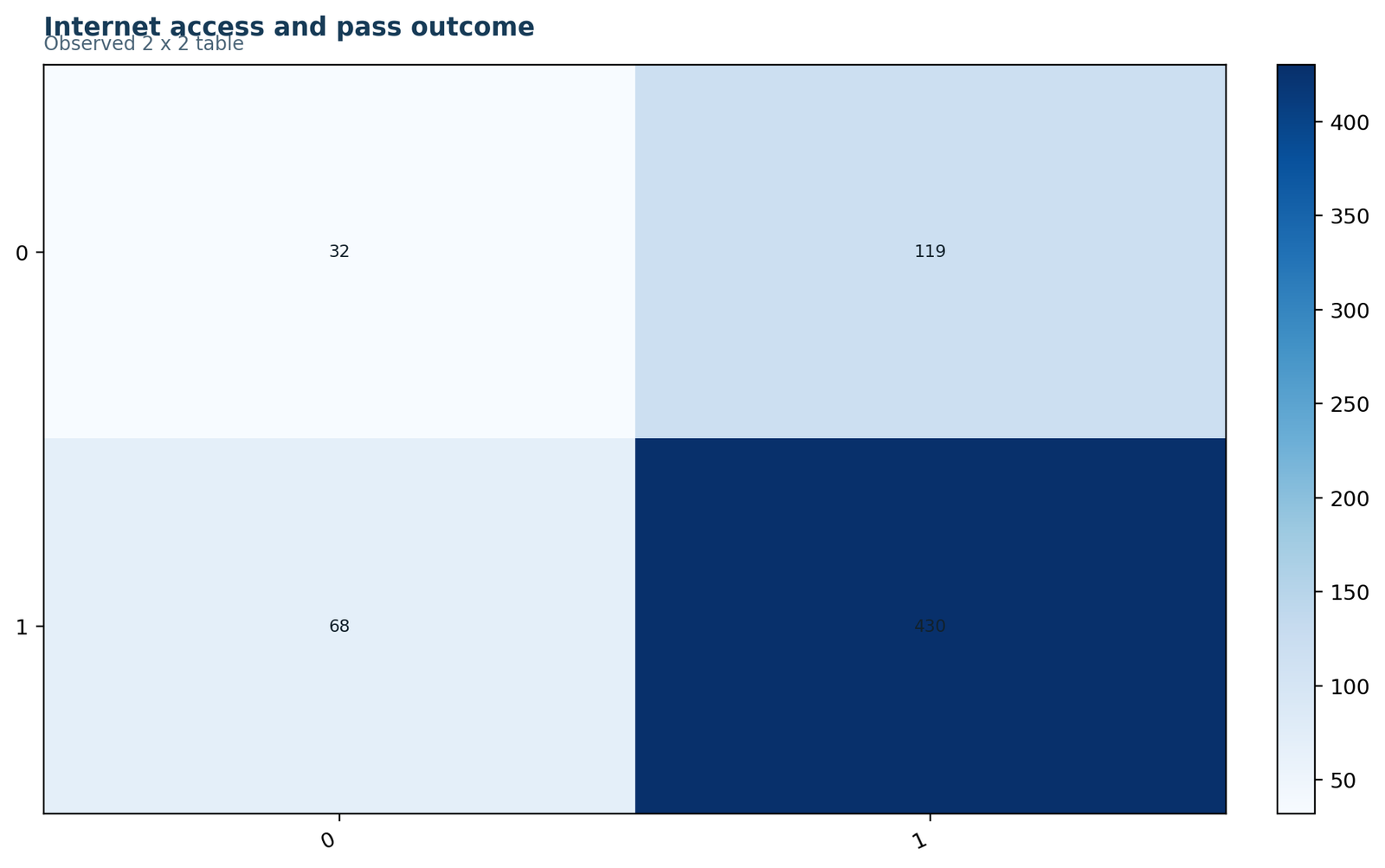
The largest cell is the exposed-pass cell: 430 students had internet access and reached G3 ≥ 10. The smallest cell is the unexposed-fail cell with 32 students.
Internet yes: 430 pass and 68 fail, n = 498. Internet no: 119 pass and 32 fail, n = 151. Total N = 649.
The table supplies the four counts a, b, c and d. The odds ratio compares the cross-products 430 × 32 and 68 × 119 rather than comparing either pair of raw counts alone.
Every odds ratio, standard error and confidence interval in the worked analysis comes from these four cells.
Python Chart 2: Odds Ratio - Group Risks and Event Percentages Python
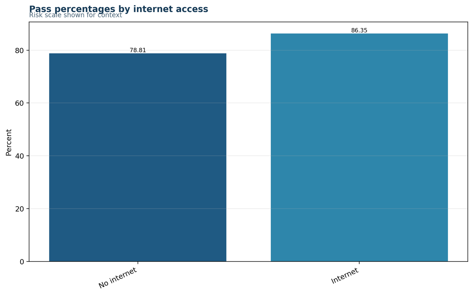
The exposed group has the higher observed pass proportion, although both groups have pass rates well above 75%.
Internet yes risk = 430/498 = 86.35%. Internet no risk = 119/151 = 78.81%. Absolute risk difference = 7.54 percentage points.
Risk and odds are related but not identical. The chart communicates probabilities, while the odds ratio is calculated from pass-to-fail odds within each exposure group.
Because the event is common, the odds ratio of 1.70 is farther from 1 than the risk ratio of approximately 1.096.
Python Chart 3: Odds Ratio - Odds Ratio with 95% Confidence Interval Python
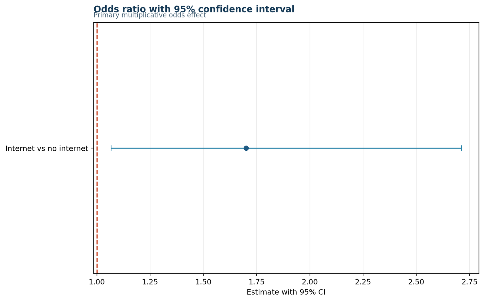
The point estimate lies above 1, and the complete log-Wald 95% confidence interval remains above 1.
OR = 1.7004. 95% CI = [1.0664, 2.7116]. Null value = 1.
The observed pass odds among students with internet access are estimated to be 1.70 times the pass odds among students without internet access. The interval indicates uncertainty in that multiplicative estimate.
An odds-ratio confidence interval is more informative than a binary significance label because it shows both direction and precision.
Python Chart 4: Odds Ratio - Log-Odds Components Python
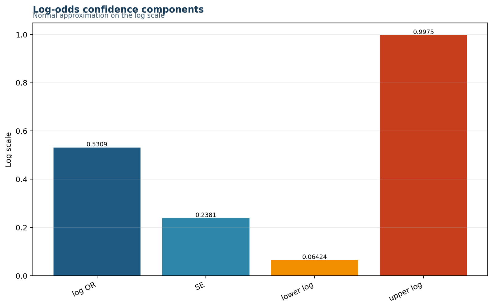
The log odds ratio is positive. The largest reciprocal-count contribution comes from the smallest cell, d = 32.
ln(OR) = 0.53089. SE[ln(OR)] = 0.23809. Reciprocal components are 1/430, 1/68, 1/119 and 1/32.
Inference is performed on the log scale because log odds ratios are approximately symmetric around zero. Exponentiation returns the estimate and interval to the odds-ratio scale.
Small cells contribute more uncertainty because their reciprocal terms are larger.
Python Chart 5: Odds Ratio - Result Summary Python
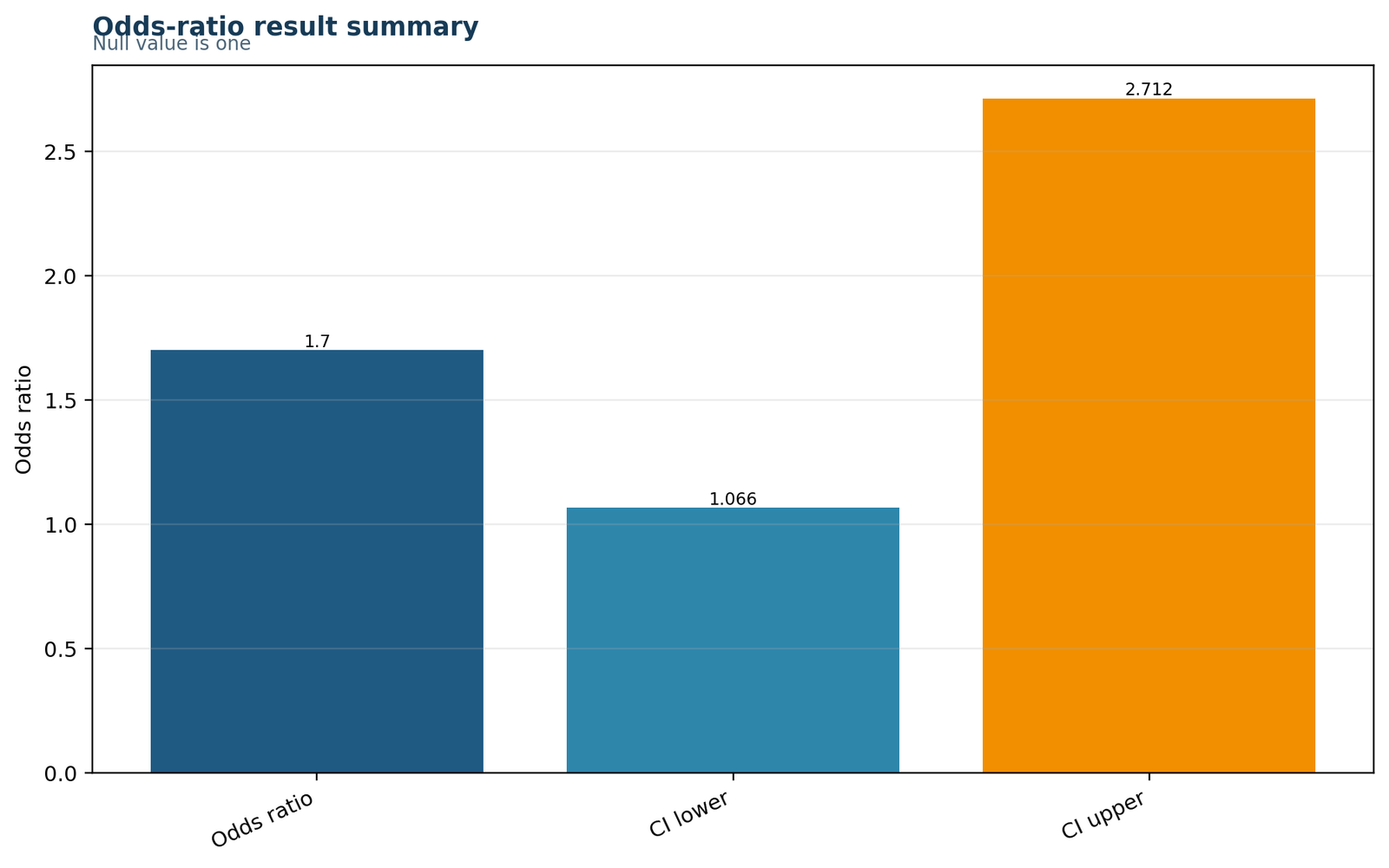
The estimate indicates higher pass odds in the internet-access group, with moderate uncertainty around the precise multiplicative value.
Exposed odds = 6.3235. Reference odds = 3.7188. OR = 1.7004. 95% CI = [1.0664, 2.7116].
The result supports a positive unadjusted association between internet access and the G3 ≥ 10 outcome in this sample. It does not establish causation or adjust for other student characteristics.
A concise summary should retain the two group definitions and the raw table context, not only the ratio.
Four Additional R Odds Ratio Charts in Two Paired Rows
The page explains nine unique chart files in total: five Python figures and four additional R-only figures. The R asset list also references the observed-table and result-summary visuals already displayed in the Python section, so those two identical files are not repeated. R coverage remains complete through the four distinct R charts below, the R workflow, expandable R code and the downloadable R report.
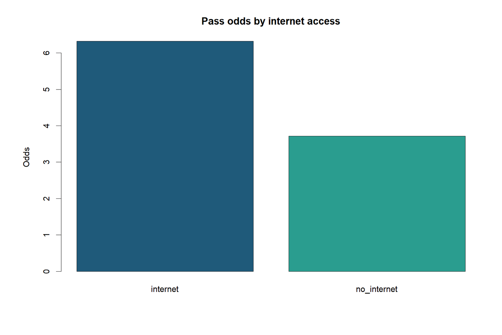
R Chart 1: Exposure-Specific Odds
Using a labelled R matrix, the pass odds are calculated as 430/68 = 6.3235 for students with internet access and 119/32 = 3.7188 for students without internet access. Their ratio is 1.7004. The chart keeps the event and reference categories visible, which helps prevent accidental inversion when a matrix is transposed or factor levels are reordered.
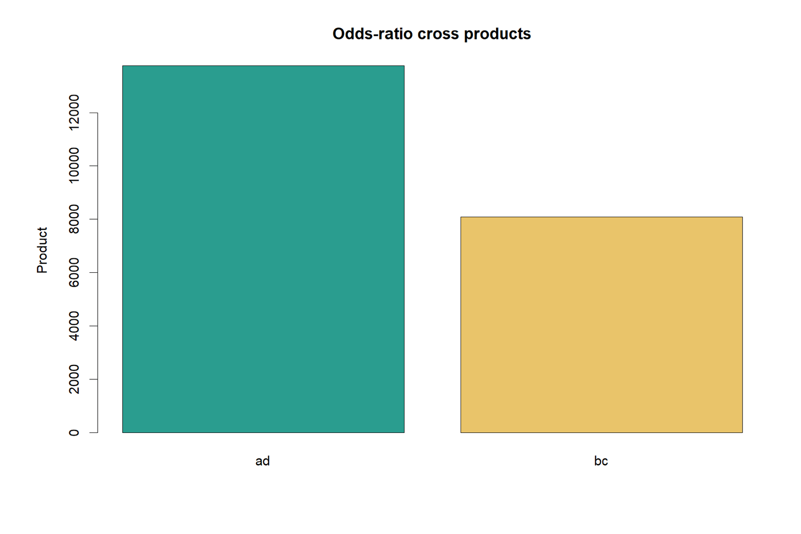
dimnames() and factor reference levels before interpreting a package-generated odds ratio.R Chart 2: Cross-Product Components
R reproduces the manual formula through a × d = 430 × 32 = 13,760 and b × c = 68 × 119 = 8,092. Dividing 13,760 by 8,092 gives OR = 1.7004. This component view is especially useful when validating package output against a direct matrix calculation.
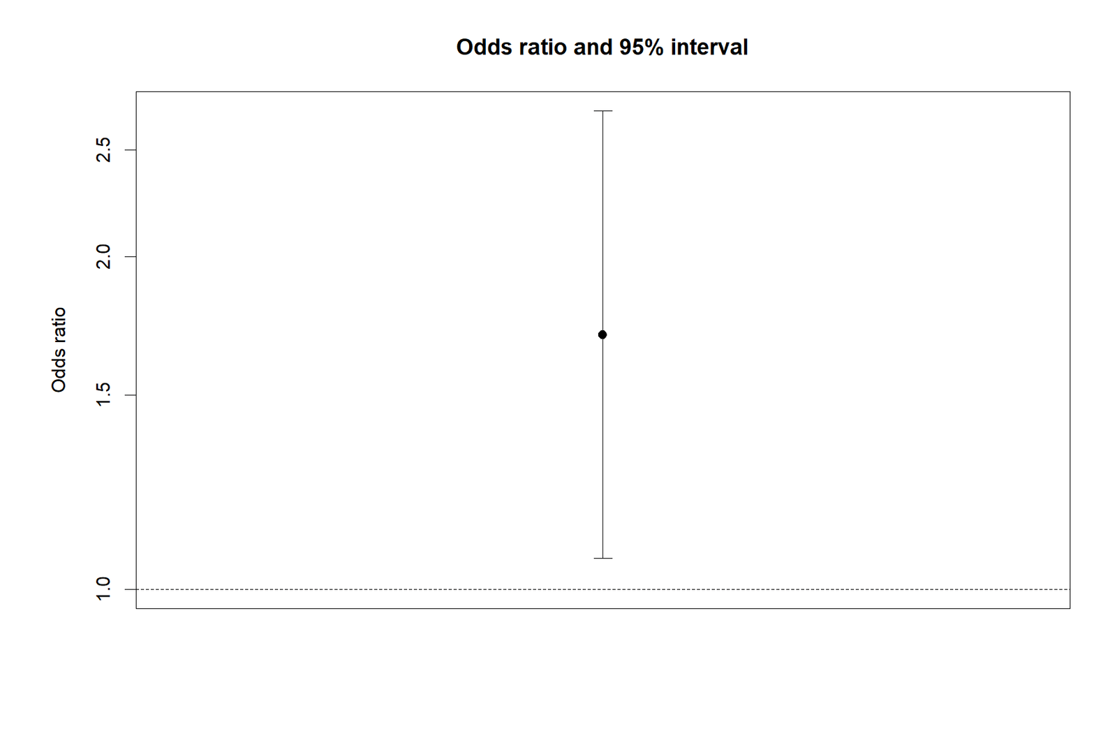
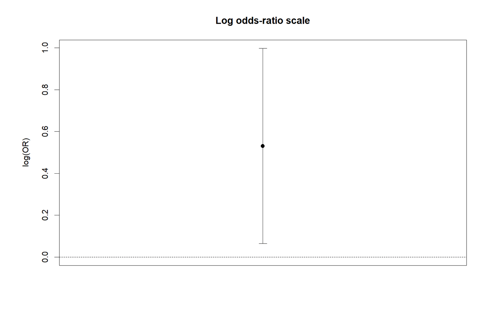
R Chart 3: Confidence Interval
The R calculation gives OR = 1.7004 with a 95% confidence interval from 1.0664 to 2.7116. Because the complete interval is above 1, the fitted unadjusted association is positive under this interval method. The width also shows that the precise multiplicative effect remains uncertain.
R Chart 4: Log-Scale View
On the log scale, ln(OR) = 0.53089 and the approximate limits are 0.06425 and 0.99753. The null value becomes zero, and equal multiplicative distances around OR = 1 become visually balanced. Exponentiating the three log values returns 1.7004 and the interval [1.0664, 2.7116].
Odds Ratio in Python, R, SPSS and Excel
Odds Ratio in Python
Python can calculate the cross-product odds ratio, log-Wald confidence interval, risks, risk ratio, risk difference and supplementary Fisher or chi-square tests from a labelled 2 × 2 array.
- Store the four counts with explicit labels.
- Calculate OR as a × d divided by b × c.
- Calculate the interval on the log scale.
- Exponentiate only after constructing the log limits.
- Use exact or penalized methods when zero cells are present.
Worked target: OR = 1.7004449 and 95% CI [1.0663594, 2.7115744].
Odds Ratio in R
R can reproduce the manual formula directly and can also obtain odds ratios through packages or logistic regression. The table orientation must remain explicit because different functions may use different row and column conventions.
- Create a 2 × 2 matrix with exposure groups in rows.
- Confirm the event column.
- Calculate the log standard error from reciprocal cells.
- Use
exp(coef(model))for logistic-regression odds ratios. - Name the interval method and package when using package-specific output.
Odds Ratio in SPSS
SPSS CROSSTABS can calculate risk estimates for a 2 × 2 table. The Risk Estimate table may show the odds ratio and relative risks, but the exact direction depends on category ordering.
- Code the exposure and outcome as binary variables.
- Request counts, row percentages and expected counts.
- Request CHISQ and RISK statistics.
- Inspect which category is displayed first.
- Report the confidence interval and category direction.
Odds Ratio in Excel
Excel can reproduce every workbook calculation with transparent formulas. Keep the four counts in clearly labelled cells and reference those cells rather than hard-coding values inside long formulas.
- Calculate the two group odds.
- Calculate the cross-product ratio.
- Use LN for the log odds ratio.
- Use SQRT for the reciprocal-count standard error.
- Use EXP to return the confidence limits to the ratio scale.
Cross-Software Reconciliation
| Quantity | Python target | R target | SPSS/Excel target |
|---|---|---|---|
| Observed table | [[430, 68], [119, 32]] | Same labelled matrix | Same four weighted or worksheet counts |
| Exposure odds | 6.3235294 | 6.3235294 | 6.3235294 |
| Reference odds | 3.7187500 | 3.7187500 | 3.7187500 |
| Odds ratio | 1.7004449 | 1.7004449 | 1.7004449 |
| 95% CI | 1.0663594–2.7115744 | 1.0663594–2.7115744 | 1.0663594–2.7115744 |
Expandable Code for the Odds Ratio
The code blocks reproduce the labelled table and the primary workbook values. They keep risks and odds separate and avoid silently changing the reference group.
Python code: odds ratio, confidence interval and supporting measures
import math
from scipy.stats import fisher_exact, chi2_contingency, norm

# Rows: internet access yes, no
# Columns: G3 >= 10, G3 < 10
a, b, c, d = 430, 68, 119, 32

odds_exposed = a / b
odds_reference = c / d
odds_ratio = (a * d) / (b * c)

log_or = math.log(odds_ratio)
se_log_or = math.sqrt(1/a + 1/b + 1/c + 1/d)
z_critical = 1.96
ci_lower = math.exp(log_or - z_critical * se_log_or)
ci_upper = math.exp(log_or + z_critical * se_log_or)

risk_exposed = a / (a + b)
risk_reference = c / (c + d)
risk_ratio = risk_exposed / risk_reference
risk_difference = risk_exposed - risk_reference

z_value = log_or / se_log_or
p_log_wald = 2 * (1 - norm.cdf(abs(z_value)))

fisher_or, fisher_p = fisher_exact([[a, b], [c, d]])
chi2, chi2_p, _, expected = chi2_contingency(
    [[a, b], [c, d]], correction=False
)

print(f"Exposed odds: {odds_exposed:.7f}")
print(f"Reference odds: {odds_reference:.7f}")
print(f"OR: {odds_ratio:.7f}")
print(f"95% CI: [{ci_lower:.7f}, {ci_upper:.7f}]")
print(f"Risk ratio: {risk_ratio:.7f}")
print(f"Risk difference: {risk_difference:.7f}")
print(f"Log-Wald p: {p_log_wald:.7f}")
print(f"Fisher p: {fisher_p:.7f}")
print(f"Pearson chi-square p: {chi2_p:.7f}")
R code: odds ratio and log-Wald confidence interval
# Rows: internet access yes, no
# Columns: G3 >= 10, G3 < 10
tab <- matrix(
  c(430, 68,
    119, 32),
  nrow = 2,
  byrow = TRUE,
  dimnames = list(
    internet = c("yes", "no"),
    outcome = c("G3_ge_10", "G3_lt_10")
  )
)

a <- tab[1, 1]
b <- tab[1, 2]
c_count <- tab[2, 1]
d <- tab[2, 2]

odds_exposed <- a / b
odds_reference <- c_count / d
odds_ratio <- (a * d) / (b * c_count)

log_or <- log(odds_ratio)
se_log_or <- sqrt(1/a + 1/b + 1/c_count + 1/d)
ci <- exp(log_or + c(-1, 1) * qnorm(0.975) * se_log_or)

risk_exposed <- a / (a + b)
risk_reference <- c_count / (c_count + d)
risk_ratio <- risk_exposed / risk_reference
risk_difference <- risk_exposed - risk_reference

list(
  table = tab,
  odds_exposed = odds_exposed,
  odds_reference = odds_reference,
  odds_ratio = odds_ratio,
  confidence_interval = ci,
  risk_ratio = risk_ratio,
  risk_difference = risk_difference,
  fisher_test = fisher.test(tab),
  chi_square = chisq.test(tab, correct = FALSE)
)
SPSS syntax: weighted 2 × 2 table with risk estimates
DATA LIST FREE /internet outcome count.
BEGIN DATA
1 1 430
1 0 68
0 1 119
0 0 32
END DATA.

VALUE LABELS internet
  1 'Internet yes'
  0 'Internet no'.
VALUE LABELS outcome
  1 'G3 at least 10'
  0 'G3 below 10'.

WEIGHT BY count.

CROSSTABS
  /TABLES=internet BY outcome
  /FORMAT=AVALUE TABLES
  /STATISTICS=CHISQ RISK PHI
  /CELLS=COUNT ROW EXPECTED
  /COUNT ROUND CELL.

WEIGHT OFF.Excel formulas for a labelled four-cell table
Assume B5 = 430, C5 = 68, B6 = 119 and C6 = 32.
Exposed odds
=B5/C5

Reference odds
=B6/C6

Odds ratio
=(B5*C6)/(C5*B6)

Log odds ratio
=LN((B5*C6)/(C5*B6))

SE of log odds ratio
=SQRT(1/B5+1/C5+1/B6+1/C6)

95% lower confidence limit
=EXP(LN((B5*C6)/(C5*B6))-NORM.S.INV(0.975)*SQRT(1/B5+1/C5+1/B6+1/C6))

95% upper confidence limit
=EXP(LN((B5*C6)/(C5*B6))+NORM.S.INV(0.975)*SQRT(1/B5+1/C5+1/B6+1/C6))

Exposed risk
=B5/SUM(B5:C5)

Reference risk
=B6/SUM(B6:C6)

Risk ratio
=(B5/SUM(B5:C5))/(B6/SUM(B6:C6))

Risk difference
=B5/SUM(B5:C5)-B6/SUM(B6:C6)
Assumptions, Limitations and Advanced Interpretation
Core Conditions
- Binary exposure or grouping variable.
- Binary event outcome.
- Mutually exclusive categories.
- Independent observations for the ordinary 2 × 2 estimate.
- Correct coding and table orientation.
- Representative or design-appropriate sampling for population inference.
- Sufficient information in all four cells for the ordinary log-Wald interval.
Interpretive Limits
- Association does not establish causation.
- Odds are not probabilities.
- A crude estimate does not adjust for confounding.
- Common outcomes can make the odds ratio look more extreme than the risk ratio.
- Selection bias and misclassification can distort the estimate.
- Collapsing a quantitative outcome loses information.
- A confidence interval does not describe the probability that the true value lies inside the observed interval.
Independence
The standard 2 × 2 formulas assume each participant contributes one independent observation. If students are nested in classes or schools, ordinary standard errors can be too small. Cluster-robust, generalized estimating equation or mixed-model methods may be needed.
Randomness and Generalizability
The arithmetic can be calculated for any four counts, but generalization depends on how the sample was obtained. Convenience sampling, nonresponse, restricted geographic coverage or selective inclusion can limit external validity.
Outcome and Exposure Misclassification
If internet access or G3 threshold status is recorded incorrectly, the odds ratio can move toward or away from 1. Nondifferential misclassification often attenuates associations under simple conditions, but that pattern is not guaranteed for every design.
Confounding
A third variable is a confounder when it is associated with the exposure and outcome and is not merely a consequence of the exposure. Prior grades, socioeconomic resources, parental education and school context may influence both internet access and achievement. Stratification or logistic regression can evaluate adjusted associations.
Effect Modification
The association may differ across subgroups. For example, the odds ratio could vary by school, prior achievement or study time. Interaction terms or stratum-specific tables can examine whether one common odds ratio is inappropriate.
Non-Collapsibility
Odds ratios can change after covariates are added even when those covariates are not classical confounders. This mathematical property means crude and adjusted odds ratios should not be compared as though every change proves confounding.
Small Samples and Sparse Cells
The ordinary log-Wald interval can perform poorly with sparse data or odds ratios far from 1. Exact conditional intervals, profile-likelihood intervals, Firth penalization or Bayesian methods may be more stable. The current table has positive cells and expected counts above 20, so the ordinary interval is computationally available.
Multiple Comparisons
Calculating many odds ratios across outcomes, exposures, thresholds or subgroups increases the chance of selecting an extreme result. A planned analysis, transparent multiplicity adjustment and complete reporting reduce selective-inference risk.
Threshold Sensitivity
The result depends on defining G3 ≥ 10 as the event. A different threshold creates a different 2 × 2 table and can change the odds ratio. The threshold should be justified before examining a collection of alternative cut points.
Sample Size and Precision
Precision depends on all four cells, not only the total N. The confidence interval widens when one or more cells are small. Prospective planning requires plausible baseline risk, exposure prevalence, target odds ratio, alpha and power.
APA Reporting for the Odds Ratio
A complete report identifies the exposure, reference group, event, cell counts or group totals, odds ratio, confidence interval and whether the estimate is crude or adjusted. P-values can be added, but they should not replace the effect estimate.
Methods Example
An unadjusted odds ratio was calculated from a 2 × 2 table to compare the odds of G3 ≥ 10 between students with internet access and students without internet access. A 95% confidence interval was calculated on the log-odds scale and exponentiated.
Results Example
Among students with internet access, 430 of 498 reached G3 ≥ 10, compared with 119 of 151 students without internet access. The odds of G3 ≥ 10 were higher in the internet-access group, OR = 1.70, 95% CI [1.07, 2.71].
Interpretation with Risk Context
The corresponding observed event risks were 86.35% and 78.81%, an absolute difference of 7.54 percentage points. The odds ratio should therefore be interpreted as a ratio of odds rather than as a 70% increase in probability.
Reporting Templates
Positive Association
CI excludes 1
In the exposure group, a of n1 participants experienced the event, compared with c of n0 in the reference group.
The event odds were higher in the exposure group, OR = estimate, 95% CI [lower, upper].
The exposure group had approximately estimate times the event odds of the reference group.
Interval Includes One
Uncertain direction
The estimated odds ratio was estimate, 95% CI [lower, upper].
The interval included 1, so the data did not provide sufficiently precise evidence of a difference in odds at the stated confidence level.
This does not prove equal odds; the interval describes the range of effects compatible with the data and method.
Adjusted Logistic-Regression Odds Ratio
Model-based
A binary logistic regression estimated the association between predictor and outcome while adjusting for covariates.
Holding the included covariates constant, the odds were multiplied by adjusted OR for a one-unit or category change in the predictor, 95% CI [lower, upper].
Reporting Checklist
- Name the odds ratio and state whether it is crude or adjusted.
- Identify the event category.
- Identify the numerator exposure group and reference group.
- Report the four counts or group event totals.
- Report OR and the confidence interval.
- Name the interval method when relevant.
- Use odds language, not probability language.
- Add risks or risk differences when they can be estimated.
- State limitations related to design and adjustment.
Common Odds Ratio Mistakes and How to Correct Them
Calculation Mistakes
- Placing counts in the wrong cells.
- Dividing risks instead of odds while calling the result an odds ratio.
- Using a + d divided by b + c.
- Failing to exponentiate log-scale limits.
- Using zero cells without an explicit method.
- Rounding cells or intermediate values too early.
- Changing the reference group without changing the interpretation.
Interpretation Mistakes
- Saying “times more likely.”
- Interpreting OR = 1.70 as a 70-percentage-point increase.
- Ignoring that the event is common.
- Claiming causation from an observational table.
- Calling a crude odds ratio adjusted.
- Reporting a p-value without an effect estimate.
- Ignoring the confidence interval width.
Mistake 1: Confusing Risk with Odds
For the internet-access group, the risk is 430/498 = 0.8635, while the odds are 430/68 = 6.3235. Both numbers describe the same group but use different denominators and have different interpretations.
Mistake 2: Reversing the Comparison
Internet yes versus no gives OR = 1.7004. Internet no versus yes gives OR = 0.5881. Both calculations can be correct, but the written interpretation must match the selected direction.
Mistake 3: Treating the Null Value as Zero
The null value for an odds ratio is 1. A confidence interval that contains 1 is compatible with equal odds. Zero is the null value for a risk difference or log odds ratio, not for the ordinary odds ratio.
Mistake 4: Calling Odds “Likelihood”
Likelihood has a separate technical meaning in statistics. “Odds” is the clearest term for the ratio p/(1 − p). In general-audience writing, also report the corresponding probability or risk.
Mistake 5: Ignoring Common Outcomes
With common events, the odds ratio can appear much larger than the risk ratio. In this example, OR = 1.7004 while RR = 1.0956. This is not an error; it reflects the different scales.
Mistake 6: Using the Simple Table When Adjustment Is Required
If the scientific question concerns an association after accounting for other variables, a crude 2 × 2 odds ratio is insufficient. Use a carefully specified logistic regression and report adjusted odds ratios.
Mistake 7: Assuming a Narrow P-Value Decision Is the Main Finding
Effect magnitude and uncertainty matter more than a standalone threshold label. The confidence interval [1.07, 2.71] shows that the estimate is positive but still compatible with a fairly broad range of multiplicative effects.
Odds Ratio Reports and Worked Excel Download
Use the software reports and worked workbook to reproduce the observed table, odds calculations, confidence interval and chart outputs.
Download R PDF ReportComplete R calculations and chart output; four unique R-only visuals are interpreted on this page.
Download SPSS PDF OutputCrosstabulation, risk estimates and association statistics.
Download Worked Excel AnalysisLabelled inputs, formulas, diagnostics and reporting values.
Frequently Asked Questions About the Odds Ratio
What is an odds ratio?
An odds ratio compares the event odds in one group with the event odds in another group. In a 2 × 2 table, it equals ad/(bc).
What is the odds ratio formula?
For cells a, b, c and d arranged as two groups by event and non-event, OR = (a/b)/(c/d) = ad/(bc).
How do I calculate an odds ratio?
Calculate event odds in each group, then divide the first group odds by the reference group odds. Equivalently, divide the two diagonal cross products.
How do I interpret an odds ratio above 1?
An odds ratio above 1 means the numerator group has higher event odds than the reference group, provided the event and group coding are stated correctly.
How do I interpret an odds ratio below 1?
An odds ratio below 1 means the numerator group has lower event odds. The percent reduction in odds is commonly described as (1 − OR) × 100%, but the result still concerns odds rather than risk.
What does an odds ratio of 1 mean?
It means the event odds are equal in the two compared groups. One is the null value for an ordinary odds ratio.
Is an odds ratio the same as relative risk?
No. An odds ratio compares odds; a relative risk compares probabilities. They can be similar for rare outcomes but can differ substantially for common outcomes.
Can I say an odds ratio of 1.70 means 70% more likely?
No. It means 70% higher odds, not necessarily 70% higher probability. Report risks or predicted probabilities when probability language is needed.
What is the confidence interval for an odds ratio?
It is a range of odds-ratio values compatible with the data and method. The ordinary interval is calculated symmetrically on the log scale and then exponentiated.
Why is the null value 1?
If the two group odds are equal, dividing one by the other gives 1. Ratio measures use 1 as the equality value.
What happens if a cell is zero?
The ordinary ratio may be zero, infinite or undefined, and the log standard error fails. A named correction or an exact, penalized or Bayesian method is needed.
What is an adjusted odds ratio?
An adjusted odds ratio comes from a model, usually logistic regression, that includes additional predictors. It is interpreted conditional on those included variables.
What is a crude odds ratio?
A crude odds ratio is the unadjusted association calculated from a single 2 × 2 table.
How is an odds ratio interpreted in logistic regression?
Exponentiating a coefficient gives the multiplicative change in odds for a one-unit predictor increase or category comparison, holding other model predictors constant.
Can an odds ratio prove causation?
No. Causal interpretation depends on design, measurement, exchangeability, positivity, consistency and appropriate adjustment, not on the ratio alone.
Should I report risk beside the odds ratio?
Yes when risk can be estimated. Group risks and risk differences make the practical magnitude easier to understand.
Is Fisher's exact test an odds ratio?
No. Fisher's exact test is a hypothesis-testing procedure for a 2 × 2 table. Its output may include an odds-ratio estimate, but the p-value and effect estimate are different quantities.
Why can crude and adjusted odds ratios differ?
They can differ because of confounding, effect modification, model specification and the non-collapsibility of the odds ratio.
Odds Ratio Conclusion
The odds ratio is a central measure for binary outcomes, 2 × 2 tables, case-control studies and logistic regression. Correct use begins with explicit coding: define the exposure group, reference group, event and non-event before calculating any ratio.
In the verified worked example, 430 of 498 students with internet access and 119 of 151 students without internet access reached G3 ≥ 10. The pass odds were 6.3235 and 3.7188, producing an unadjusted odds ratio of 1.7004 with a 95% confidence interval from 1.0664 to 2.7116.
The most accurate interpretation is that the observed pass odds were approximately 1.70 times as high in the internet-access group. Because the event was common, the odds ratio should not be translated directly into a probability increase. Reporting the two risks and the 7.54-percentage-point risk difference provides essential context.

