
.rd-wrap{–ink:#172033;–muted:#607083;–navy:#123b5d;–blue:#176ea6;–teal:#087f6b;–amber:#b86b10;–rose:#a33a54;–line:#d8e3ea;–soft:#f5f9fc;–soft2:#eefbf8;–warn:#fff7e8;–danger:#fff1f2;–code:#101828;max-width:1120px;margin:0 auto;color:var(–ink);font-family:system-ui,-apple-system,BlinkMacSystemFont,”Segoe UI”,Arial,sans-serif;line-height:1.76}
.rd-wrap *{box-sizing:border-box}.rd-wrap h1,.rd-wrap h2,.rd-wrap h3,.rd-wrap h4{line-height:1.25}.rd-wrap h2{font-size:30px;color:var(–navy);margin:0 0 16px}.rd-wrap h3{font-size:23px;color:#245877;margin:28px 0 12px}.rd-wrap h4{font-size:18px;color:#263c52;margin:22px 0 9px}.rd-wrap p{margin:0 0 16px}.rd-wrap a{color:#0b6598;text-decoration:underline}.rd-wrap li{margin:7px 0}
.rd-hero{padding:36px;border:1px solid var(–line);border-radius:26px;background:linear-gradient(135deg,#eef7fb 0%,#fff 52%,#fff4e7 100%);box-shadow:0 14px 36px rgba(24,59,86,.08);margin:14px 0 26px}
.rd-kicker{display:inline-flex;align-items:center;gap:8px;padding:7px 13px;border-radius:999px;background:#e7f6f3;border:1px solid #bce5dc;color:#075f52;font-size:13px;font-weight:800;letter-spacing:.04em;text-transform:uppercase;margin-bottom:15px}
.rd-hero h1{font-size:43px;color:#102e46;margin:0 0 16px}.rd-hero p{font-size:20px;color:#2b3b4e;margin:0}.rd-badges{display:flex;flex-wrap:wrap;gap:10px;margin-top:22px}.rd-badge{padding:8px 12px;border-radius:999px;border:1px solid var(–line);background:#fff;font-weight:750;font-size:14px}
.rd-ad{padding:18px;border:1px dashed #aebbc8;border-radius:16px;text-align:center;color:#718096;background:#fcfdfe;margin:27px 0}.rd-ad span{display:block;font-size:11px;text-transform:uppercase;letter-spacing:.1em;margin-bottom:4px}
.rd-section{background:#fff;border:1px solid var(–line);border-radius:22px;padding:25px;margin:24px 0;box-shadow:0 8px 24px rgba(15,23,42,.035)}
.rd-note{background:#f5f9fd;border-left:5px solid var(–navy);border-radius:16px;padding:18px 20px;margin:19px 0}.rd-success{background:#ecfdf5;border:1px solid #bbf7d0;border-radius:17px;padding:18px 20px;margin:19px 0}.rd-warning{background:var(–warn);border:1px solid #f1d19b;border-radius:17px;padding:18px 20px;margin:19px 0}.rd-danger{background:var(–danger);border:1px solid #fecdd3;border-radius:17px;padding:18px 20px;margin:19px 0}
.rd-stat-grid{display:grid;grid-template-columns:repeat(4,minmax(0,1fr));gap:14px;margin:20px 0}.rd-stat{padding:17px;border:1px solid var(–line);border-radius:17px;background:var(–soft)}.rd-stat small{display:block;color:var(–muted);margin-bottom:6px}.rd-stat strong{display:block;font-size:23px;color:var(–navy)}
.rd-result-grid{display:grid;grid-template-columns:1fr 1fr;gap:18px;margin:20px 0}.rd-result{border:1px solid var(–line);border-radius:19px;padding:20px}.rd-result.method{background:#f1f8fc}.rd-result.meaning{background:#f0fbf7}.rd-result h3{margin:0 0 8px}.rd-result ul{margin:10px 0 0;padding-left:20px}
.rd-toc{columns:2;column-gap:34px;margin:0;padding-left:20px}.rd-toc li{break-inside:avoid;margin:8px 0}
.rd-problem-grid{display:grid;grid-template-columns:repeat(3,minmax(0,1fr));gap:15px}.rd-problem{border:1px solid var(–line);border-radius:18px;padding:18px;background:var(–soft)}.rd-problem strong{display:block;font-size:20px;color:var(–navy);margin-bottom:5px}.rd-problem span{color:var(–muted)}
.rd-flow{display:grid;grid-template-columns:1fr auto 1fr auto 1fr;gap:12px;align-items:stretch;margin:22px 0}.rd-step{border:1px solid var(–line);border-radius:18px;padding:19px;background:#fff}.rd-step b{display:block;color:var(–teal);font-size:13px;text-transform:uppercase;letter-spacing:.05em;margin-bottom:7px}.rd-arrow{display:flex;align-items:center;font-size:28px;color:#8aa0b2;font-weight:800}
.rd-formula{padding:18px;border:1px solid var(–line);border-radius:17px;text-align:center;background:#f7f9fc;font-weight:800;font-size:19px;color:var(–navy);margin:18px 0;overflow-x:auto}
.rd-table-wrap{overflow-x:auto;border:1px solid var(–line);border-radius:18px;margin:18px 0}.rd-table{width:100%;min-width:880px;border-collapse:collapse;background:#fff}.rd-table th{background:#edf5f9;color:#163d58;text-align:left;padding:12px;border-bottom:1px solid var(–line)}.rd-table td{padding:12px;border-bottom:1px solid #edf1f4;vertical-align:top}.rd-table tr:last-child td{border-bottom:none}
.rd-decision-grid{display:grid;grid-template-columns:repeat(2,minmax(0,1fr));gap:16px;margin:20px 0}.rd-decision{border:1px solid var(–line);border-radius:18px;padding:19px;background:#fff}.rd-decision h3{margin-top:0}.rd-decision.use{border-top:5px solid var(–teal)}.rd-decision.avoid{border-top:5px solid var(–amber)}
.rd-method-grid{display:grid;grid-template-columns:repeat(4,minmax(0,1fr));gap:13px;margin:20px 0}.rd-method{border:1px solid var(–line);border-radius:17px;padding:17px;background:#fff}.rd-method strong{display:block;color:var(–navy);font-size:18px;margin-bottom:7px}.rd-method p{font-size:14px;color:#405368;margin:0}
.rd-chart-story{border-top:1px solid var(–line);padding:30px 0 8px}.rd-chart-story:first-of-type{border-top:none;padding-top:4px}.rd-figure{margin:16px 0 18px;border:1px solid var(–line);border-radius:20px;overflow:hidden;background:#fff}.rd-figure img{display:block;width:100%;height:auto}.rd-figure figcaption{padding:13px 16px;background:#fbfdff;border-top:1px solid var(–line);color:var(–muted);font-size:14px}
.rd-insight-grid{display:grid;grid-template-columns:1fr 1fr;gap:13px}.rd-insight{border:1px solid var(–line);border-radius:16px;padding:16px;background:#fff}.rd-insight span{display:block;font-size:12px;font-weight:850;letter-spacing:.06em;text-transform:uppercase;color:var(–teal);margin-bottom:7px}.rd-insight p{margin:0}.rd-next{margin:13px 0 0;padding:13px 15px;border-radius:14px;background:#f3f7fb;color:#405368;font-size:14px}
.rd-metric-grid{display:grid;grid-template-columns:repeat(3,minmax(0,1fr));gap:14px}.rd-metric{border:1px solid var(–line);border-radius:17px;padding:17px;background:#fff}.rd-metric b{display:block;color:var(–navy);margin-bottom:6px}.rd-metric strong{font-size:20px;color:var(–teal)}
.rd-software-grid{display:grid;grid-template-columns:repeat(2,minmax(0,1fr));gap:16px}.rd-software{border:1px solid var(–line);border-radius:18px;padding:19px}.rd-software h3{margin:0 0 8px}.rd-software ul{padding-left:19px;margin:8px 0}
.rd-details details{border:1px solid var(–line);border-radius:15px;padding:14px 16px;margin:11px 0;background:#fff}.rd-details summary{cursor:pointer;font-weight:850;color:var(–navy)}.rd-details details>div{padding-top:13px}
.rd-code{background:var(–code);color:#e5e7eb;border-radius:17px;padding:17px;overflow-x:auto;font-size:13.5px;line-height:1.62}.rd-code code{font-family:Consolas,Monaco,”Courier New”,monospace}
.rd-two-col{display:grid;grid-template-columns:1fr 1fr;gap:18px}.rd-list-card{border:1px solid var(–line);border-radius:18px;padding:19px;background:#fff}.rd-list-card h3{margin:0 0 9px}.rd-list-card ul{padding-left:20px;margin:0}
.rd-apa-grid{display:grid;grid-template-columns:1fr 1fr;gap:16px;margin:18px 0}.rd-report{border:1px solid var(–line);border-radius:18px;padding:19px;background:#fff}.rd-report h3{margin:0 0 10px}.rd-copy{border-left:5px solid var(–teal);background:#f0fbf7;border-radius:15px;padding:17px 19px;margin:14px 0}.rd-copy p:last-child{margin-bottom:0}.rd-template{border:1px dashed #9fb0bf;border-radius:15px;background:#fbfdff;padding:16px;margin:12px 0}.rd-template code{white-space:normal;color:#20364a;font-family:inherit}
.rd-r-pair{margin:28px 0 34px;padding:20px;border:1px solid var(–line);border-radius:21px;background:#fbfdff}.rd-r-pair-title{margin:0 0 15px;font-size:17px;color:var(–navy);font-weight:850}.rd-r-chart-row{display:grid;grid-template-columns:repeat(2,minmax(0,1fr));gap:18px;align-items:start}.rd-r-chart-box{border:1px solid var(–line);border-radius:18px;overflow:hidden;background:#fff}.rd-r-chart-box figure{margin:0}.rd-r-chart-box img{display:block;width:100%;height:auto}.rd-r-chart-box figcaption{padding:12px 14px;background:#f7fafc;border-top:1px solid var(–line);color:var(–muted);font-size:13px}.rd-r-explanation-row{display:grid;grid-template-columns:repeat(2,minmax(0,1fr));gap:18px;margin-top:14px}.rd-r-explanation{border:1px solid var(–line);border-radius:17px;padding:17px;background:#fff}.rd-r-explanation h3{font-size:19px;margin:0 0 9px}.rd-r-label{display:block;font-size:12px;font-weight:850;letter-spacing:.06em;text-transform:uppercase;color:var(–teal);margin-bottom:6px}.rd-r-check{padding:11px 13px;border-radius:13px;background:#eef7fb;color:#405368;font-size:13px;margin-top:10px}
.rd-download-grid{display:grid;grid-template-columns:repeat(2,minmax(0,1fr));gap:14px}.rd-download{display:block;text-decoration:none!important;border:1px solid var(–line);border-radius:17px;padding:18px;background:#fff}.rd-download strong{display:block;color:var(–navy);font-size:18px;margin-bottom:5px}.rd-download span{color:var(–muted);font-size:14px}.rd-related{display:grid;grid-template-columns:repeat(2,minmax(0,1fr));gap:11px}.rd-related a{display:block;padding:12px 14px;border:1px solid var(–line);border-radius:14px;background:#f8fafc;text-decoration:none}.rd-faq details{border:1px solid var(–line);border-radius:15px;padding:15px 17px;margin:10px 0}.rd-faq summary{cursor:pointer;font-weight:850;color:var(–navy)}.rd-faq p{margin-top:11px}
html{scroll-behavior:smooth}.rd-top-anchor{position:absolute;top:0;left:0;width:1px;height:1px;overflow:hidden}.rd-back-to-top{position:fixed;right:22px;bottom:24px;width:48px;height:48px;display:flex;align-items:center;justify-content:center;border-radius:50%;background:var(–navy);color:#fff!important;text-decoration:none!important;font-size:25px;font-weight:900;box-shadow:0 10px 24px rgba(15,23,42,.24);z-index:9999;border:2px solid rgba(255,255,255,.85)}.rd-back-to-top:hover{background:var(–teal);transform:translateY(-3px)}.rd-back-to-top span{position:absolute;width:1px;height:1px;overflow:hidden;clip:rect(0,0,0,0)}
@media(max-width:900px){.rd-method-grid{grid-template-columns:repeat(2,1fr)}.rd-stat-grid,.rd-metric-grid{grid-template-columns:repeat(2,1fr)}.rd-result-grid,.rd-two-col,.rd-software-grid,.rd-download-grid,.rd-related,.rd-insight-grid,.rd-apa-grid,.rd-decision-grid,.rd-r-chart-row,.rd-r-explanation-row{grid-template-columns:1fr}.rd-flow{grid-template-columns:1fr}.rd-arrow{justify-content:center;transform:rotate(90deg)}.rd-toc{columns:1}.rd-problem-grid{grid-template-columns:1fr}.rd-hero h1{font-size:34px}}
@media(max-width:540px){.rd-stat-grid,.rd-metric-grid,.rd-method-grid{grid-template-columns:1fr}.rd-section,.rd-hero{padding:21px}.rd-hero h1{font-size:29px}.rd-hero p{font-size:17px}.rd-wrap h2{font-size:25px}.rd-back-to-top{right:15px;bottom:18px;width:44px;height:44px}}
/* Readable APA templates: deliberately avoid theme styling. */
.rd-template{
border:1px dashed #9fb0bf!important;
border-radius:15px!important;
background:#fbfdff!important;
padding:17px 19px!important;
margin:13px 0 20px!important;
color:#20364a!important;
box-shadow:none!important;
}
.rd-template,
.rd-template *{
color:#20364a!important;
background:transparent!important;
text-shadow:none!important;
box-shadow:none!important;
}
.rd-template-text{
display:block!important;
margin:0!important;
padding:0!important;
border:0!important;
font-family:system-ui,-apple-system,BlinkMacSystemFont,"Segoe UI",Arial,sans-serif!important;
font-size:16px!important;
font-weight:400!important;
line-height:1.78!important;
white-space:normal!important;
word-break:normal!important;
overflow-wrap:anywhere!important;
}
/* Final APA reporting cards */
.rd-apa-template-intro{
display:flex;
align-items:flex-start;
gap:12px;
padding:15px 17px;
margin:16px 0 18px;
border:1px solid #c9d9e5;
border-radius:15px;
background:#f5faff;
color:#29435a
}
.rd-apa-template-intro strong{color:var(--navy)}
.rd-apa-template-grid{
display:grid;
grid-template-columns:repeat(2,minmax(0,1fr));
gap:16px;
margin:16px 0 24px
}
.rd-apa-template-card{
border:1px solid var(--line);
border-radius:19px;
padding:19px;
background:#fff;
box-shadow:0 5px 16px rgba(15,23,42,.035)
}
.rd-apa-template-card.directional{grid-column:1/-1}
.rd-apa-template-head{
display:flex;
flex-wrap:wrap;
align-items:center;
gap:10px;
margin-bottom:13px
}
.rd-apa-template-head h4{
margin:0;
color:var(--navy);
font-size:20px
}
.rd-apa-status{
display:inline-flex;
align-items:center;
border-radius:999px;
padding:5px 10px;
font-size:12px;
line-height:1.2;
font-weight:850;
letter-spacing:.035em;
text-transform:uppercase
}
.rd-apa-status.ns{background:#eef4f8;color:#39556b;border:1px solid #cbd8e1}
.rd-apa-status.sig{background:#ecfdf5;color:#076451;border:1px solid #b7e8da}
.rd-apa-status.one{background:#fff7e8;color:#8a520a;border:1px solid #efcf98}
.rd-apa-template-copy{
border-left:5px solid var(--blue);
border-radius:14px;
background:#f8fbfe;
padding:16px 17px;
color:#20364a
}
.rd-apa-template-card.sig-card .rd-apa-template-copy{border-left-color:var(--teal)}
.rd-apa-template-card.directional .rd-apa-template-copy{border-left-color:var(--amber)}
.rd-apa-template-copy p{
margin:0 0 11px!important;
color:#20364a!important;
font-size:16px!important;
line-height:1.72!important
}
.rd-apa-template-copy p:last-child{margin-bottom:0!important}
.rd-slot{
display:inline-block;
border:1px solid #b9d2e3;
border-radius:7px;
background:#eaf5fc;
color:#164e72;
padding:1px 6px;
margin:1px 1px;
font-weight:750;
white-space:nowrap
}
.rd-apa-template-card.sig-card .rd-slot{
border-color:#b6dfd4;
background:#eaf9f5;
color:#086653
}
.rd-apa-template-card.directional .rd-slot{
border-color:#e3c68d;
background:#fff5df;
color:#87510b
}
.rd-template-tip{
display:block;
margin-top:11px;
color:var(--muted);
font-size:13px
}
/* One presentation for charts shared by Python and R */
.rd-cross-software{
padding:16px 18px;
border:1px solid #c8dfd8;
border-radius:16px;
background:#f0fbf7;
margin:16px 0 22px;
color:#284b43
}
.rd-chart-badge{
display:inline-flex;
margin-left:8px;
padding:4px 9px;
border-radius:999px;
border:1px solid #c8d8e3;
background:#f3f8fb;
color:#36566d;
font-size:11px;
font-weight:800;
letter-spacing:.035em;
text-transform:uppercase;
vertical-align:middle
}
@media(max-width:850px){
.rd-apa-template-grid{grid-template-columns:1fr}
.rd-apa-template-card.directional{grid-column:auto}
}
/* Final robust APA-template layout */
.rd-apa-template-grid{display:block!important;margin:16px 0 24px!important}
.rd-apa-template-card,.rd-apa-template-card.directional{
display:block!important;width:100%!important;grid-column:auto!important;
margin:0 0 18px!important;padding:20px!important;overflow:visible!important
}
.rd-apa-template-head{
display:flex!important;align-items:center!important;flex-wrap:wrap!important;
gap:10px!important;margin:0 0 13px!important
}
.rd-apa-template-head h4{margin:0!important;font-size:21px!important;line-height:1.3!important}
.rd-apa-template-copy{display:block!important;width:100%!important;padding:4px 17px!important}
.rd-template-row{
display:grid!important;grid-template-columns:118px minmax(0,1fr)!important;
gap:14px!important;align-items:start!important;padding:13px 0!important;
border-bottom:1px solid #dce7ee!important
}
.rd-template-row:last-child{border-bottom:0!important}
.rd-template-label{
display:block!important;color:#31566f!important;font-size:12px!important;
line-height:1.35!important;font-weight:800!important;letter-spacing:.055em!important;
text-transform:uppercase!important;padding-top:4px!important
}
.rd-template-row p{
display:block!important;margin:0!important;color:#20364a!important;
font-size:16px!important;line-height:1.75!important;min-width:0!important
}
.rd-field{
display:inline!important;padding:1px 4px!important;border-radius:4px!important;
background:#eaf5fc!important;color:#145274!important;font-weight:750!important;
box-decoration-break:clone;-webkit-box-decoration-break:clone
}
.rd-apa-template-card.sig-card .rd-field{background:#eaf9f5!important;color:#086653!important}
.rd-apa-template-card.directional .rd-field{background:#fff3d9!important;color:#81500c!important}
.rd-template-tip{
display:block!important;margin-top:12px!important;padding-top:11px!important;
border-top:1px dashed #cbd9e2!important;color:var(--muted)!important;font-size:13px!important
}
@media(max-width:650px){
.rd-template-row{grid-template-columns:1fr!important;gap:5px!important}
.rd-template-label{padding-top:0!important}
}
.rd-kpi-strip{display:grid;grid-template-columns:repeat(5,minmax(0,1fr));gap:12px;margin:18px 0}.rd-kpi{border:1px solid var(--line);border-radius:16px;padding:15px;background:#fff}.rd-kpi small{display:block;color:var(--muted);margin-bottom:5px}.rd-kpi strong{display:block;color:var(--navy);font-size:20px}.rd-math{font-family:Georgia,"Times New Roman",serif}.rd-calc-grid{display:grid;grid-template-columns:repeat(4,minmax(0,1fr));gap:12px;margin:16px 0}.rd-calc-cell{border:1px solid var(--line);border-radius:15px;padding:15px;background:#f8fbfd}.rd-calc-cell span{display:block;color:var(--muted);font-size:13px}.rd-calc-cell strong{display:block;color:var(--navy);font-size:20px;margin-top:4px}.rd-mini-grid{display:grid;grid-template-columns:repeat(3,minmax(0,1fr));gap:13px}.rd-mini{border:1px solid var(--line);border-radius:16px;padding:16px;background:#fff}.rd-mini h4{margin:0 0 7px}.rd-mini p{margin:0}.rd-practice{counter-reset:item}.rd-practice-card{border:1px solid var(--line);border-radius:17px;padding:18px;margin:14px 0;background:#fff}.rd-practice-card h3{margin:0 0 9px}.rd-answer{margin-top:12px;padding:14px 16px;border-radius:14px;background:#f0fbf7;border:1px solid #c5e7dd}.rd-keyword-note{border-left:5px solid var(--blue);background:#f4f9fd;border-radius:14px;padding:16px 18px;margin:16px 0}.rd-checklist{display:grid;grid-template-columns:repeat(2,minmax(0,1fr));gap:12px}.rd-check{border:1px solid var(--line);border-radius:15px;padding:14px;background:#fff}.rd-check strong{display:block;color:var(--navy);margin-bottom:4px}.rd-check span{color:var(--muted)}
@media(max-width:900px){.rd-kpi-strip,.rd-calc-grid,.rd-mini-grid,.rd-checklist{grid-template-columns:1fr 1fr}}
@media(max-width:540px){.rd-kpi-strip,.rd-calc-grid,.rd-mini-grid,.rd-checklist{grid-template-columns:1fr}}
.rd-key-grid{display:grid;grid-template-columns:repeat(3,minmax(0,1fr));gap:14px;margin:18px 0}.rd-key{border:1px solid var(--line);border-radius:17px;padding:17px;background:#fff}.rd-key b{display:block;color:var(--navy);margin-bottom:6px}.rd-key strong{font-size:21px;color:var(--teal)}
.rd-calc-grid{display:grid;grid-template-columns:repeat(4,minmax(0,1fr));gap:13px;margin:18px 0}.rd-calc{border:1px solid var(--line);border-radius:16px;padding:16px;background:#f8fbfd}.rd-calc b{display:block;color:var(--navy);margin-bottom:5px}.rd-calc span{color:var(--muted);font-size:14px}
.rd-answer{border:1px solid #c9d9e5;border-radius:15px;padding:16px 18px;background:#f7fbfe;margin:12px 0}.rd-answer strong{color:var(--navy)}
.rd-mini{font-size:14px;color:var(--muted)}
.rd-nowrap{white-space:nowrap}
@media(max-width:900px){.rd-key-grid,.rd-calc-grid{grid-template-columns:repeat(2,1fr)}}
@media(max-width:540px){.rd-key-grid,.rd-calc-grid{grid-template-columns:1fr}}
.rd-inline-chart{border:1px solid var(--line);border-radius:20px;padding:22px;background:#fff;margin:16px 0 18px}.rd-bar-row{display:grid;grid-template-columns:180px minmax(0,1fr) 74px;gap:12px;align-items:center;margin:15px 0}.rd-bar-label{font-weight:800;color:var(--navy)}.rd-bar-track{height:24px;background:#edf3f7;border-radius:999px;overflow:hidden;border:1px solid #d7e2ea}.rd-bar-fill{height:100%;background:linear-gradient(90deg,var(--blue),var(--teal));border-radius:999px}.rd-bar-value{text-align:right;font-weight:850;color:var(--navy)}.rd-inline-caption{margin:13px 0 0;color:var(--muted);font-size:14px}.rd-summary-visual{padding:18px;background:#fff}.rd-summary-visual .rd-stat-grid{margin:0}.rd-summary-visual .rd-stat strong{font-size:20px}@media(max-width:540px){.rd-bar-row{grid-template-columns:1fr}.rd-bar-value{text-align:left}.rd-bar-track{height:20px}}
.rd-band-grid{display:grid;grid-template-columns:repeat(4,minmax(0,1fr));gap:12px;margin:18px 0}.rd-band{border:1px solid var(--line);border-radius:16px;padding:16px;background:#fff}.rd-band b{display:block;color:var(--navy);margin-bottom:5px}.rd-band span{font-size:14px;color:var(--muted)}
.rd-equation-stack{display:grid;grid-template-columns:1fr 1fr;gap:15px}.rd-equation-card{border:1px solid var(--line);border-radius:17px;padding:17px;background:#f8fbfd}.rd-equation-card h4{margin-top:0}.rd-mini{font-size:14px;color:var(--muted)}
.rd-link-note{padding:15px 17px;border:1px solid #c9dce8;border-radius:15px;background:#f6fbff;margin:15px 0}
.rd-check-grid{display:grid;grid-template-columns:repeat(3,minmax(0,1fr));gap:14px}.rd-check{border:1px solid var(--line);border-radius:17px;padding:17px;background:#fff}.rd-check strong{display:block;color:var(--navy);margin-bottom:7px}
@media(max-width:900px){.rd-band-grid,.rd-check-grid{grid-template-columns:repeat(2,1fr)}.rd-equation-stack{grid-template-columns:1fr}}
@media(max-width:540px){.rd-band-grid,.rd-check-grid{grid-template-columns:1fr}}
.rd-emphasis{font-weight:850;color:var(--navy)}
.rd-number-negative{color:#9f2942!important}.rd-number-positive{color:#087f6b!important}
.rd-scale-row{display:grid;grid-template-columns:160px 1fr;gap:14px;padding:13px 0;border-bottom:1px solid var(--line)}
.rd-scale-row:last-child{border-bottom:none}.rd-scale-row b{color:var(--navy)}
.rd-data-note{font-size:14px;color:var(--muted);margin-top:8px}
@media(max-width:620px){.rd-scale-row{grid-template-columns:1fr;gap:4px}}
Risk Difference: Formula, Interpretation, Example, Confidence Interval, Python, R, SPSS and Excel Guide
This worked Risk Difference guide measures the absolute change in G3 pass probability associated with paid classes. It uses all 649 records, preserves the exact 2 × 2 counts, calculates Wald and Newcombe confidence intervals, analyses the raw G3 distribution, tests threshold sensitivity, reconciles Python, R, SPSS and Excel outputs, and explains what the negative estimate does—and does not—show.
Risk Difference Model Overview
Risk difference is the exposed-group probability minus the reference-group probability. It is also called the absolute risk difference, risk difference measure, rate difference in some incidence settings, or absolute percentage-point effect when both probabilities refer to the same follow-up period. Unlike a ratio, risk difference remains on the original probability scale.
The worked design defines paid classes = yes as group 1 and paid classes = no as group 0. The event is a final-grade pass, coded as G3 ≥ 10. The source data contain 39 paid-class students and 610 students without paid classes. The observed pass counts are 30 and 519, respectively.
The Exact Analytical Question
How many more or fewer students pass per 100 when the paid-class group is compared with the no-paid-class group in this dataset?
Quick Answer: Risk Difference Result
The absolute risk difference is obtained by subtracting the no-paid-class pass probability from the paid-class pass probability. The sign is negative because 76.92% is below 85.08%.
Statistical Decision
- Primary measure: absolute risk difference
- Estimate: −0.081589
- Newcombe 95% CI: −0.236394 to 0.027080
- Null value: 0
- Decision: the 95% interval includes no difference
Data Meaning
- 30 of 39 paid-class students passed.
- 519 of 610 students without paid classes passed.
- The observed gap equals about 8 fewer passes per 100.
- The interval permits a decrease as large as 23.64 points.
- It also permits a small increase up to 2.71 points.
Table of Contents
- What risk difference means
- Research question and hypotheses
- When to use risk difference
- Risk-difference variants and scales
- Variables and data dictionary
- Formula and manual calculation
- Observed data and G3 profiles
- Complete results and diagnostics
- Assumptions and design checks
- Risk difference versus related measures
- Calculator workflow
- Python chart interpretations
- Paired R chart interpretations
- Python, R, SPSS and Excel workflows
- Expandable code
- Interpretation and APA reporting
- Common mistakes
- Practice questions
- Reports and worked files
- Related guides
- Frequently asked questions
- Conclusion
What Is Risk Difference?
Risk difference is an additive effect measure for a binary outcome. If p1 is the risk in group 1 and p0 is the risk in group 0, then RD = p1 − p0. A value of zero means equal observed risks. Positive values indicate more events in group 1; negative values indicate fewer events in group 1.
Why the Additive Scale Matters
Decision-makers often need the absolute number of outcomes associated with an exposure or intervention. A risk ratio says how many times as likely an event is; a risk difference says how many additional or fewer events occur per 100 or per 1,000 people. In this dataset, RD = −0.081589 corresponds to approximately 81.59 fewer passes per 1,000 paid-class students compared with the no-paid-class risk, if the sample estimate were transported without adjustment.
Direction Depends on Coding
What Risk Difference Does Not Prove
Risk difference describes an observed association. It does not prove causation, eliminate confounding, adjust for baseline differences, or guarantee that the same absolute effect applies in another population. The difference is especially vulnerable to selection when exposure is self-chosen rather than randomized. Review experimental versus quasi-experimental design and sampling bias before making causal claims.
Research Question, Hypotheses and Data Design
Research Question
In the observed student data, how different is the G3 pass probability for students reporting paid classes compared with students reporting no paid classes?
Null and Alternative Hypotheses
| Component | Statement | Meaning |
|---|---|---|
| Null hypothesis | H0: ppaid − pno = 0 | The two groups have the same pass probability. |
| Two-sided alternative | H1: ppaid − pno ≠ 0 | The absolute pass probabilities differ in either direction. |
| Directional interpretation | RD < 0 under current coding | The paid-class group has a lower observed pass probability. |
Design Facts That Control Interpretation
- Exposure is observational and self-reported.
- The paid-class group is small: 39 of 649 students, or 6.01%.
- The reference group contains 610 students.
- The event threshold is fixed at G3 ≥ 10 in the workbook.
- Every student contributes once to one exposure group and one outcome.
When to Use Risk Difference
Use Risk Difference When
- The outcome is binary.
- Two independent groups are compared.
- Absolute change is more useful than a ratio alone.
- Probabilities refer to a common time horizon or assessment point.
- Counts and denominators are available.
- Public-health, clinical, educational or policy decisions require events per 100 or 1,000.
- A confidence interval can be reported.
- The group and event coding are explicit.
Use Another Method or Extension When
- Outcomes are paired or repeated on the same people.
- Follow-up times differ substantially and incidence rates are required.
- Multiple confounders need adjustment.
- Clustered or survey data require design-based standard errors.
- The outcome has more than two categories.
- Risks vary by important subgroups and one pooled difference hides interaction.
- Very sparse counts require exact or specialized methods.
- The target is causal rather than descriptive association.
Decision Flow
Create a valid event/non-event definition before calculation.
Use paired methods for matched or repeated observations.
Report risk difference, then add ratio measures for context if needed.
For binary cross-tabulations and expected-count checks, see cross-tabulation, chi-square test of independence and Fisher’s exact test.
Risk Difference Variants and Interpretation Scales
The phrase “risk difference” can describe several closely related estimands. The formula must match the design and outcome timing.
Difference between two observed cumulative probabilities at one defined assessment point.
Difference between covariate-standardized predicted probabilities from a suitable model.
Difference in incidence rates when person-time rather than persons is the denominator.
Absolute difference for matched or repeated binary outcomes with dependence handled explicitly.
| Scale | Worked value | Interpretation |
|---|---|---|
| Probability scale | -0.081589 | The paid-class pass probability is lower by 0.081589. |
| Percentage-point scale | -8.1589 points | About 8.16 fewer passes per 100. |
| Per-1,000 scale | -81.59 per 1,000 | About 81.59 fewer passes per 1,000. |
| Reverse comparison | 0.081589 | No-paid-class minus paid-class risk. |
| Failure outcome | 0.081589 | Paid-class failure risk minus no-paid-class failure risk. |
Negative Risk Difference
Yes, risk difference can be negative. Under the current coding, a negative value means the event is less common in group 1. Whether that is beneficial or harmful depends on the event. Here the event is passing, so a negative value is adverse for the paid-class group. If the event were failure, the same underlying table would produce a positive risk difference.
Variables, Coding and Data Dictionary
| Variable | Role | Coding | Valid N | Meaning |
|---|---|---|---|---|
| paid | Exposure/group variable | yes = group 1; no = group 0 | 649 | Indicates whether the student reported paid classes. |
| G3 | Original quantitative outcome | 0 to 19 in the observed data | 649 | Final grade retained for descriptive and sensitivity analysis. |
| G3 pass | Derived binary event | 1 if G3 ≥ 10; 0 otherwise | 649 | Outcome used in the 2 × 2 risk-difference calculation. |
Group Composition
| Group | N | Sample share | Pass | Fail | Pass risk |
|---|---|---|---|---|---|
| Paid classes = yes | 39 | 6.01% | 30 | 9 | 76.92% |
| Paid classes = no | 610 | 93.99% | 519 | 91 | 85.08% |
| Full sample | 649 | 100.00% | 549 | 100 | 84.59% |
Raw G3 Descriptive Statistics
| Group | N | Mean | Median | SD | Q1 | Q3 | Range |
|---|---|---|---|---|---|---|---|
| Paid classes = yes | 39 | 11.2051 | 12.0 | 2.8486 | 10.0 | 13.0 | 0–16 |
| Paid classes = no | 610 | 11.9508 | 12.0 | 3.2505 | 10.0 | 14.0 | 0–19 |
The raw-grade comparison supports the direction of the binary result: the paid-class mean is 11.21 versus 11.95, and the upper quartile is 13 versus 14. The medians are both 12, showing that the binary difference is not a complete summary of the two distributions.
Risk Difference Formula and Manual Calculation
Arrange the counts so group 1 is the first row and the event is the first outcome column.
| Pass | Fail | Total | |
|---|---|---|---|
| Paid classes = yes | 30 | 9 | 39 |
| Paid classes = no | 519 | 91 | 610 |
| Column total | 549 | 100 | 649 |
Step 1: Calculate the Group Risks
Step 2: Subtract in the Declared Direction
Multiplying by 100 gives -8.1589 percentage points.
Step 3: Wald Standard Error
| Variance component | Value | Share of total |
|---|---|---|
| Paid-class component | 0.004551661 | 95.63% |
| No-paid-class component | 0.000208075 | 4.37% |
| Total variance | 0.004759736 | 100.00% |
The paid-class component contributes 95.63% of the Wald variance because n = 39 is much smaller than n = 610. Increasing the reference group further would have limited effect unless the paid-class group also increased.
Step 4: Wald 95% Confidence Interval
Step 5: Newcombe 95% Confidence Interval
The workbook uses Wilson intervals for each group and then combines the one-sided distances. This avoids relying entirely on the symmetric Wald approximation.
| Component | Lower | Estimate | Upper |
|---|---|---|---|
| Paid-class Wilson interval | 0.616637 | 0.769231 | 0.873542 |
| No-paid-class Wilson interval | 0.820355 | 0.850820 | 0.876893 |
| Risk-difference Newcombe interval | -0.236394 | -0.081589 | 0.027080 |
Observed Data, Outcome Counts and G3 Profiles
Observed 2 × 2 Table
| Paid classes | Pass (G3 ≥ 10) | Fail (G3 < 10) | Row total | Row pass % |
|---|---|---|---|---|
| Yes | 30 | 9 | 39 | 76.92% |
| No | 519 | 91 | 610 | 85.08% |
| Total | 549 | 100 | 649 | 84.59% |
Outcome Count Reconciliation
| Check | Calculation | Result |
|---|---|---|
| Paid total | 30 + 9 | 39 |
| No-paid total | 519 + 91 | 610 |
| Pass total | 30 + 519 | 549 |
| Fail total | 9 + 91 | 100 |
| Grand total | 39 + 610 | 649 |
Complete G3 Distribution by Paid-Class Status
| G3 score | Paid count | Paid % | No-paid count | No-paid % |
|---|---|---|---|---|
| 0 | 1 | 2.56% | 14 | 2.30% |
| 1 | 0 | 0.00% | 1 | 0.16% |
| 2 | 0 | 0.00% | 0 | 0.00% |
| 3 | 0 | 0.00% | 0 | 0.00% |
| 4 | 0 | 0.00% | 0 | 0.00% |
| 5 | 0 | 0.00% | 1 | 0.16% |
| 6 | 0 | 0.00% | 3 | 0.49% |
| 7 | 1 | 2.56% | 9 | 1.48% |
| 8 | 3 | 7.69% | 32 | 5.25% |
| 9 | 4 | 10.26% | 31 | 5.08% |
| 10 | 3 | 7.69% | 94 | 15.41% |
| 11 | 7 | 17.95% | 97 | 15.90% |
| 12 | 8 | 20.51% | 64 | 10.49% |
| 13 | 7 | 17.95% | 75 | 12.30% |
| 14 | 1 | 2.56% | 62 | 10.16% |
| 15 | 2 | 5.13% | 47 | 7.70% |
| 16 | 2 | 5.13% | 34 | 5.57% |
| 17 | 0 | 0.00% | 29 | 4.75% |
| 18 | 0 | 0.00% | 15 | 2.46% |
| 19 | 0 | 0.00% | 2 | 0.33% |
Zeros are retained because the table is a full audit of all integer G3 values observed from 0 through 19.
Threshold Sensitivity
The primary event is G3 ≥ 10. The following table shows how the absolute difference changes when the pass threshold is moved. This is a descriptive sensitivity analysis, not permission to choose the threshold that produces the most favorable result.
| Pass definition | Paid passes | Paid risk | No-paid passes | No-paid risk | Risk difference |
|---|---|---|---|---|---|
| G3 ≥ 8 | 37/39 | 94.87% | 582/610 | 95.41% | -0.54 points |
| G3 ≥ 9 | 34/39 | 87.18% | 550/610 | 90.16% | -2.98 points |
| G3 ≥ 10 | 30/39 | 76.92% | 519/610 | 85.08% | -8.16 points |
| G3 ≥ 11 | 27/39 | 69.23% | 425/610 | 69.67% | -0.44 points |
| G3 ≥ 12 | 20/39 | 51.28% | 328/610 | 53.77% | -2.49 points |
| G3 ≥ 13 | 12/39 | 30.77% | 264/610 | 43.28% | -12.51 points |
| G3 ≥ 14 | 5/39 | 12.82% | 189/610 | 30.98% | -18.16 points |
| G3 ≥ 15 | 4/39 | 10.26% | 127/610 | 20.82% | -10.56 points |
Complete Risk Difference Results and Data Diagnostics
Paid minus no-paid pass probability
Absolute difference per 100
Lower 95% compatibility limit
Upper 95% compatibility limit
Supplementary relative scale
Supplementary odds scale
Primary Results Table
| Measure | Estimate | 95% interval or reference | Interpretation |
|---|---|---|---|
| Paid-class risk | 0.769231 | Wilson 0.616637 to 0.873542 | 30 passes among 39 students. |
| No-paid-class risk | 0.850820 | Wilson 0.820355 to 0.876893 | 519 passes among 610 students. |
| Risk difference | -0.081589 | Newcombe -0.236394 to 0.027080 | Observed absolute pass-probability difference. |
| Risk difference | -8.1589 points | -23.6394 to 2.7080 points | Percentage-point presentation. |
| Null value | 0 | Contained in the Newcombe interval | No clear two-sided difference at the 95% level. |
Wald and Newcombe Interval Comparison
| Method | Lower | Estimate | Upper | Width |
|---|---|---|---|---|
| Wald | -0.216811 | -0.081589 | 0.053633 | 0.270444 |
| Newcombe | -0.236394 | -0.081589 | 0.027080 | 0.263474 |
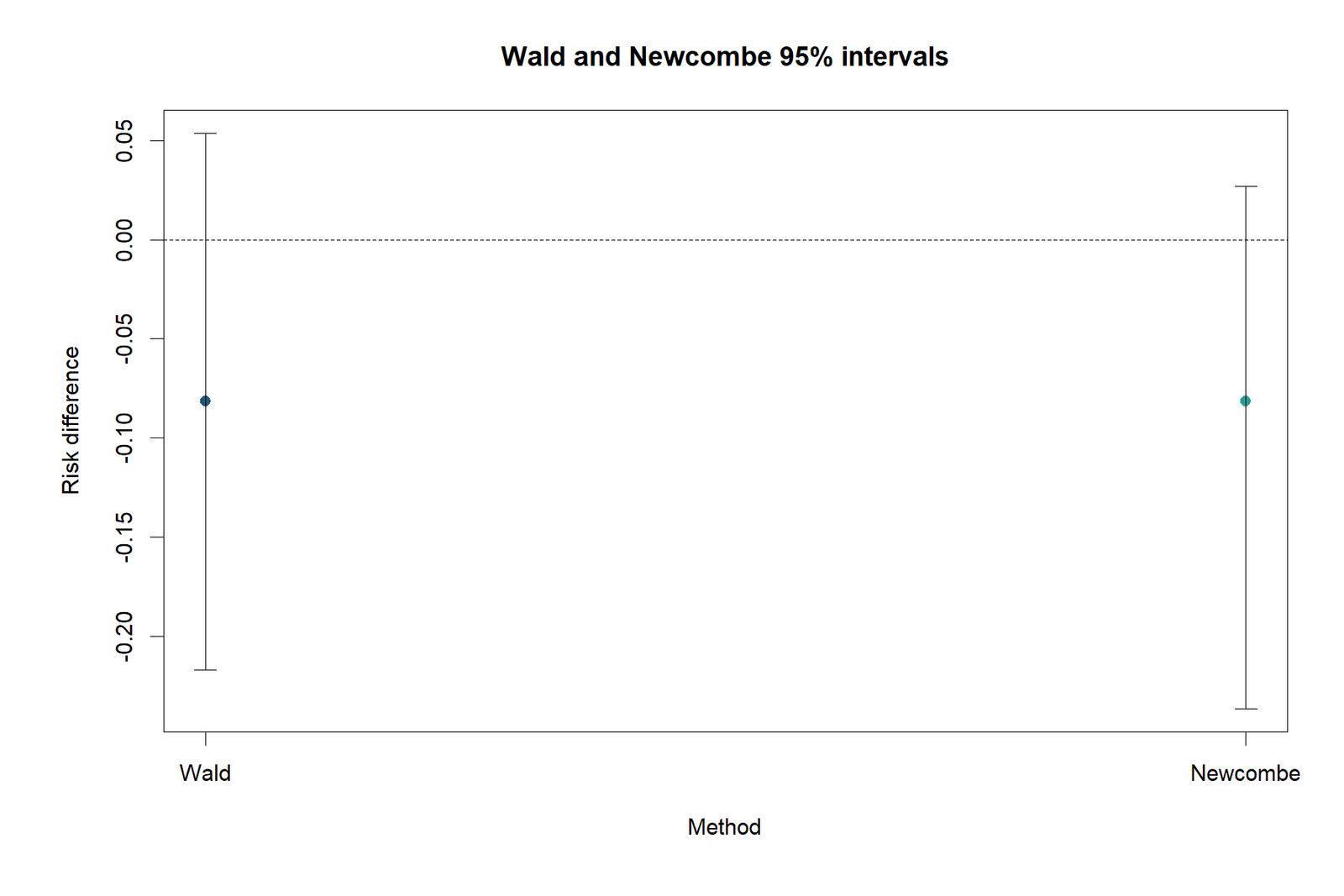
Both intervals cross zero. The Newcombe interval is wider and asymmetric around the estimate because it inherits the unequal Wilson uncertainty of the two group risks.
Expected Counts Under Equal Group Risk
| Cell | Observed | Expected | Pearson residual |
|---|---|---|---|
| Paid × pass | 30 | 32.991 | -0.521 |
| Paid × fail | 9 | 6.009 | 1.220 |
| No paid × pass | 519 | 516.009 | 0.132 |
| No paid × fail | 91 | 93.991 | -0.308 |
The largest Pearson residual is +1.22 in the paid-class failure cell. None exceeds ±2, which is consistent with the confidence interval crossing zero. These residuals describe the table composition; the Newcombe interval remains the primary inferential summary.
Supplementary Scale Translation
| Measure | Value | Data-based meaning |
|---|---|---|
| Risk ratio | 0.9041 | The paid-class pass risk is 90.41% of the no-paid-class pass risk. |
| Relative risk reduction in passing | 9.59% | A relative decrease, not an absolute percentage-point decrease. |
| Odds ratio | 0.5845 | The pass odds are lower in the paid-class group. |
| Descriptive reciprocal |1/RD| | 12.26 | Roughly one fewer pass per 12.26 students if the point estimate were causal and transportable; the interval does not support a stable NNH. |
Risk Difference Assumptions and Diagnostic Checks
Risk difference itself is a descriptive contrast, but interval interpretation depends on the design and sampling process. The following checks are more important than mechanically applying one formula.
G3 pass is coded 1 for G3 ≥ 10 and 0 otherwise.
Each student appears once in one paid-class group.
Paid yes minus paid no is declared before interpreting the sign.
G3 is measured at the same final-grade stage for both groups.
Both groups contain passes and failures.
The Newcombe interval accompanies the estimate.
Observed Diagnostic Summary
| Check | Observed evidence | Implication |
|---|---|---|
| Group size | 39 paid versus 610 no paid | Strong imbalance; precision is governed by the paid group. |
| Event counts | 30/39 and 519/610 | No zero cells; direct calculation is defined. |
| Smallest expected cell | 6.009 | Above 5, though the paid group remains small. |
| Variance share | 95.63% from paid group | More paid-group observations would most improve precision. |
| Interval includes zero | -0.2364 to 0.0271 | Direction is uncertain at the 95% level. |
| Threshold sensitivity | RD ranges from −0.44 to −18.16 points across shown thresholds | Magnitude depends on the event definition. |
Confounding and Selection
Paid classes are not randomly assigned. Students who are struggling may be more likely to seek paid instruction, creating confounding by indication. Socioeconomic access, prior grades, school, study time and family support may also influence both exposure and outcome. An adjusted analysis could use binary logistic regression followed by standardized predicted probabilities, but the simple workbook deliberately reports the unadjusted absolute contrast.
Generalizability
The estimate is sample-specific. Transporting −8.16 points to another school system assumes comparable exposure definitions, outcome thresholds, student characteristics and selection mechanisms. Those assumptions are not established by the 2 × 2 table.
Risk Difference Versus Related Measures
| Measure | Formula | Null value | Worked value | Main use |
|---|---|---|---|---|
| Risk difference | p₁ − p₀ | 0 | -0.0816 | Absolute events gained or lost. |
| Risk ratio | p₁ / p₀ | 1 | 0.9041 | Relative probability comparison. |
| Odds ratio | [p₁/(1−p₁)] / [p₀/(1−p₀)] | 1 | 0.5845 | Odds-based association; common in logistic models. |
| Pearson chi-square | Σ(O−E)²/E | 0 association | Not the primary effect measure | Tests independence but does not give absolute magnitude. |
Risk Difference Versus Relative Measures
The same table produces an 8.16-point absolute decrease, a risk ratio of 0.9041 and an odds ratio of 0.5845. These numbers are not interchangeable. The odds ratio appears more extreme because odds and probabilities diverge when the event is common. With pass risks near 77% and 85%, the odds ratio should not be described as a risk ratio.
Risk Difference Versus Percentage Change
A decrease from 85.08% to 76.92% is an 8.16 percentage-point decrease. Relative to the 85.08% reference risk, it is a 9.59% relative decrease. Writing “8.16% lower” is ambiguous unless the scale is identified.
Risk Difference Versus Chi-Square or Fisher’s Exact Test
A significance test asks whether the table is compatible with independence; risk difference asks how large the absolute contrast is. A strong report may include both, but effect magnitude and confidence limits should remain central. See chi-square test, Fisher’s exact test and odds ratio.
Risk Difference Calculator: Step-by-Step Workflow
A reliable risk difference calculator should require four counts and make the group direction visible. The following workflow reproduces the workbook.
Pass a = 30; fail b = 9.
Pass c = 519; fail d = 91.
Paid yes minus paid no.
Calculator Audit Table
| Input or output | Formula | Worked value |
|---|---|---|
| Group 1 total | a + b | 39 |
| Group 0 total | c + d | 610 |
| Group 1 risk | a/(a+b) | 0.769230769 |
| Group 0 risk | c/(c+d) | 0.850819672 |
| Risk difference | p₁−p₀ | -0.081588903 |
| Percentage points | 100×RD | -8.158890 |
| Wald SE | Square-root variance formula | 0.068990840 |
| Newcombe lower | Wilson-combination formula | -0.236393781 |
| Newcombe upper | Wilson-combination formula | 0.027079852 |
Excel Cell Logic
| Task | Example formula |
|---|---|
| Paid risk | =B5/D5 |
| No-paid risk | =B6/D6 |
| Risk difference | =B5/D5-B6/D6 |
| Wald SE | =SQRT((B5/D5)*(1-B5/D5)/D5+(B6/D6)*(1-B6/D6)/D6) |
| Wald lower | =RD-1.96*SE |
| Wald upper | =RD+1.96*SE |
Python Risk Difference Chart Interpretations
The six Python figures translate the 2 × 2 table into risks, intervals, component uncertainty, outcome counts and the final absolute-effect summary. Every chart is interpreted with the exact workbook values.
Python Chart 1: Risk Difference Observed 2 × 2 Table
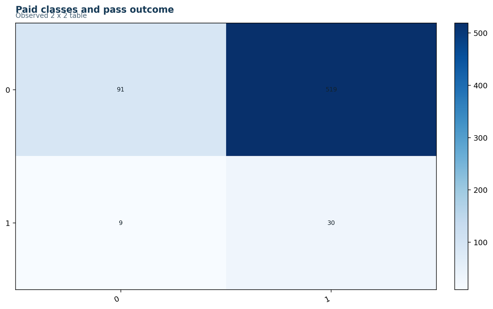
The no-paid group dominates the table numerically, with 610 students versus 39 in the paid group.
Paid: 30 pass and 9 fail. No paid: 519 pass and 91 fail.
Counts alone are not comparable because denominators differ; row risks must be calculated.
A transposed table or reversed event column would change the meaning and potentially the sign.
Python Chart 2: Risk Difference Group Risks
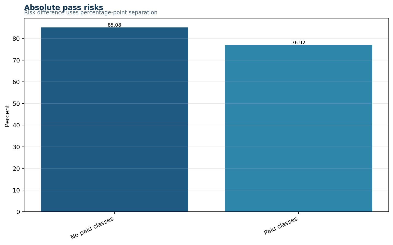
The paid-class risk bar is lower than the no-paid-class bar.
Paid = 0.769231; no paid = 0.850820; vertical gap = 0.081589.
The observed absolute pass-probability difference is −8.16 percentage points.
Showing both risks prevents an isolated effect estimate from hiding the baseline risk.
Python Chart 3: Risk Difference Confidence Intervals
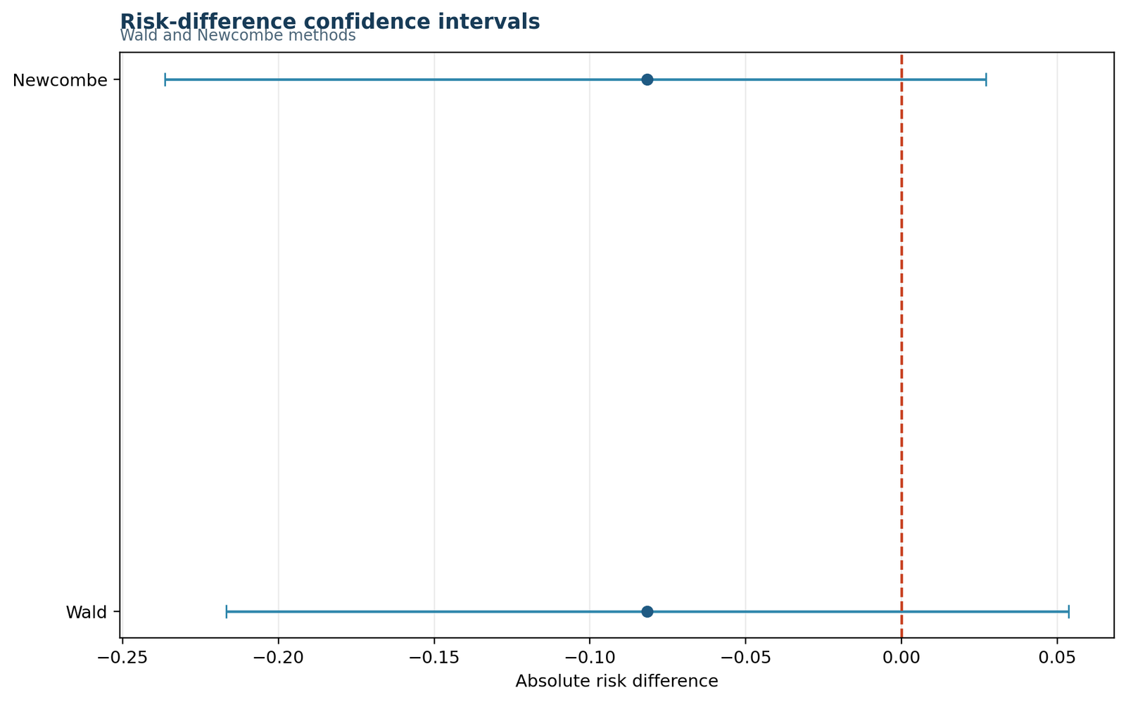
The paid-group interval is much wider because n = 39.
Paid Wilson: 0.6166–0.8735; no-paid Wilson: 0.8204–0.8769; RD Newcombe: −0.2364–0.0271.
The risk-difference interval crosses zero, so the observed negative direction is not resolved at 95% confidence.
Precision is dominated by the small paid-class group rather than the large reference group.
Python Chart 4: Risk Difference Effect Components
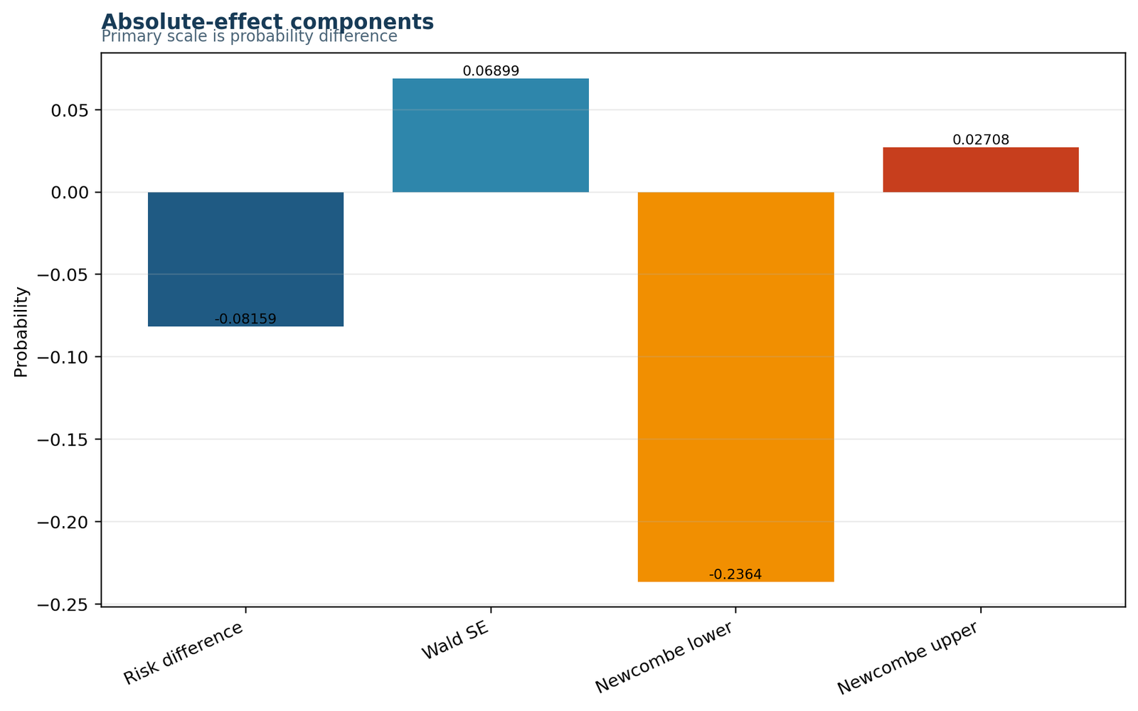
The absolute gap is modest compared with the uncertainty attached to group 1.
RD = -0.081589; SE = 0.068991; paid variance share = 95.63%.
Most interval width originates from the paid-group binomial variance.
A much larger reference sample cannot compensate fully for a small exposed sample.
Python Chart 5: Risk Difference Outcome Counts
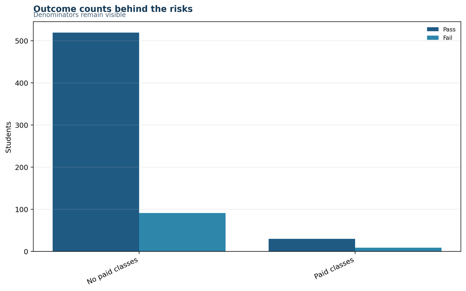
Passes are the majority in both groups; failures are relatively more common in the paid group.
Paid failure risk = 9/39 = 23.08%; no-paid failure risk = 91/610 = 14.92%.
The failure-risk difference is +8.16 points, the sign-reversed counterpart of the pass-risk difference.
Outcome coding changes the sign but not the underlying information in a binary table.
Python Chart 6: Risk Difference Result Summary
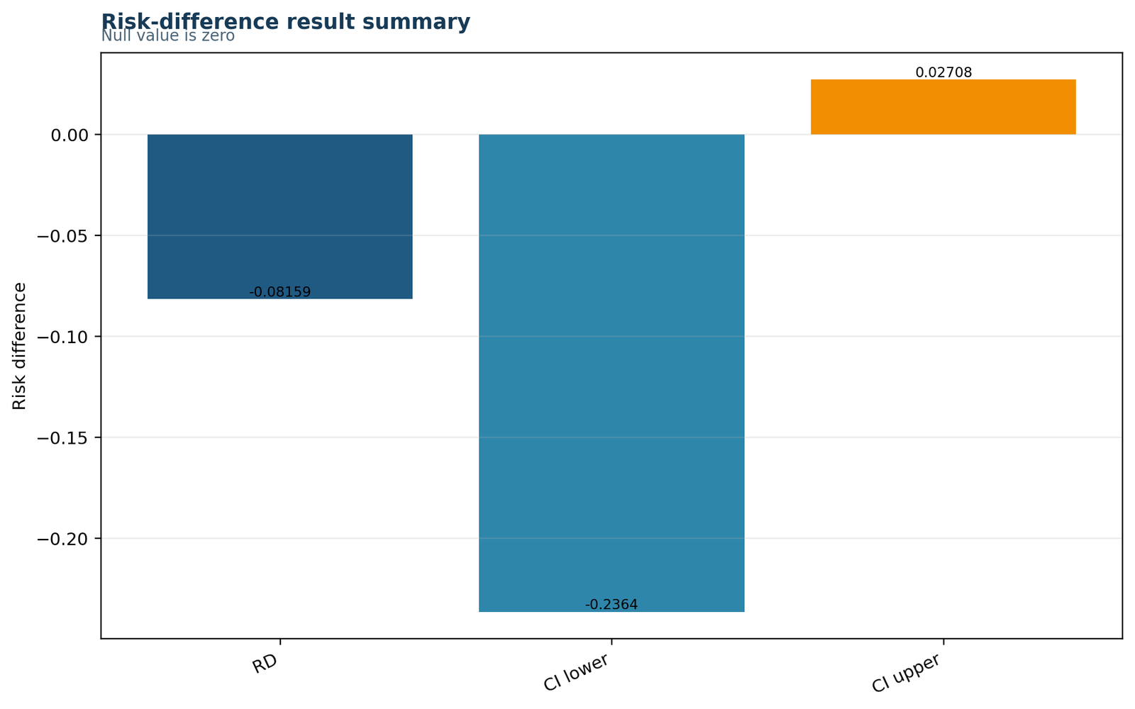
The point estimate is below zero and the upper confidence limit is slightly above zero.
RD = −0.081589; 95% CI = −0.236394 to 0.027080.
The most compatible values include a meaningful decrease, no effect and a small increase.
The confidence interval conveys both direction and uncertainty more completely than a binary significance label.
R Risk Difference Charts in Paired Rows
The R figures are arranged in three horizontal pairs on desktop and collapse to one column on mobile. The pair structure keeps each visual beside the analytical check needed to interpret it.
Observed Table
The observed table confirms 30/9 in the paid group and 519/91 in the no-paid group. The denominators differ sharply, so raw bar heights must not be interpreted as risks.
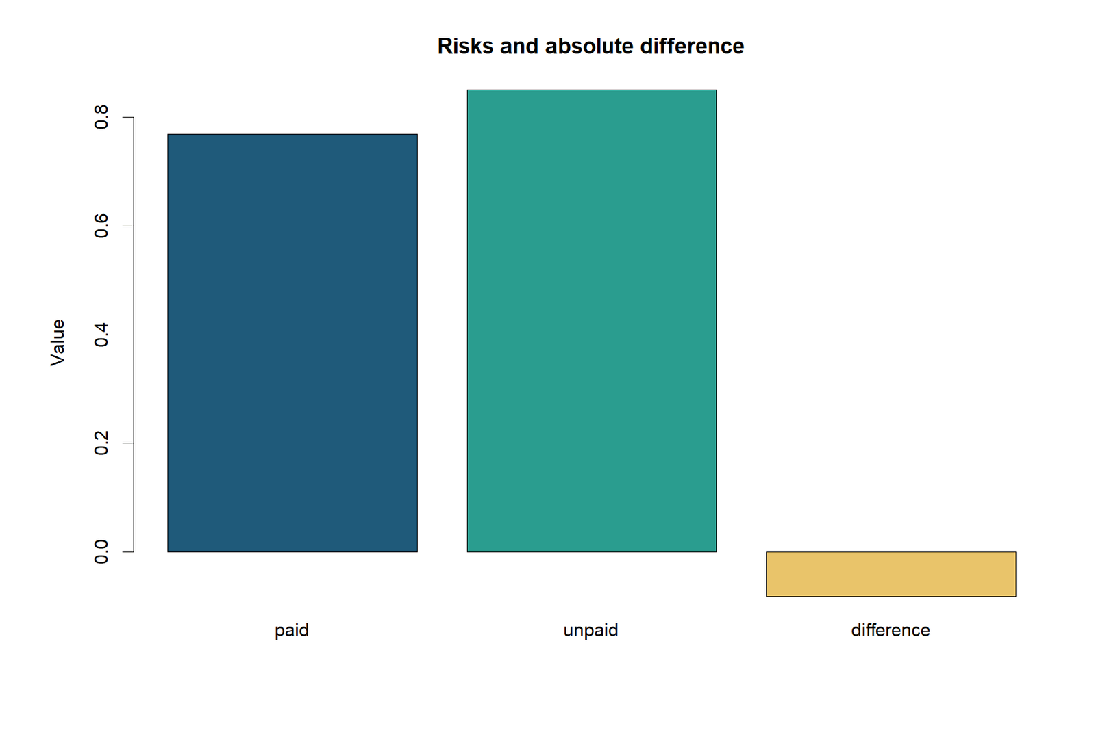
Group Risks
The R risk plot reproduces 76.92% and 85.08%. The 8.16-point vertical separation is the absolute effect estimate.
Absolute Difference
The point at −0.081589 lies below the zero reference line. Its sign reflects paid yes minus paid no, not a universal direction.
Confidence Intervals
The Newcombe interval extends from −0.236394 to 0.027080 and crosses zero. The wider paid-group uncertainty is visible beside the narrow no-paid interval.
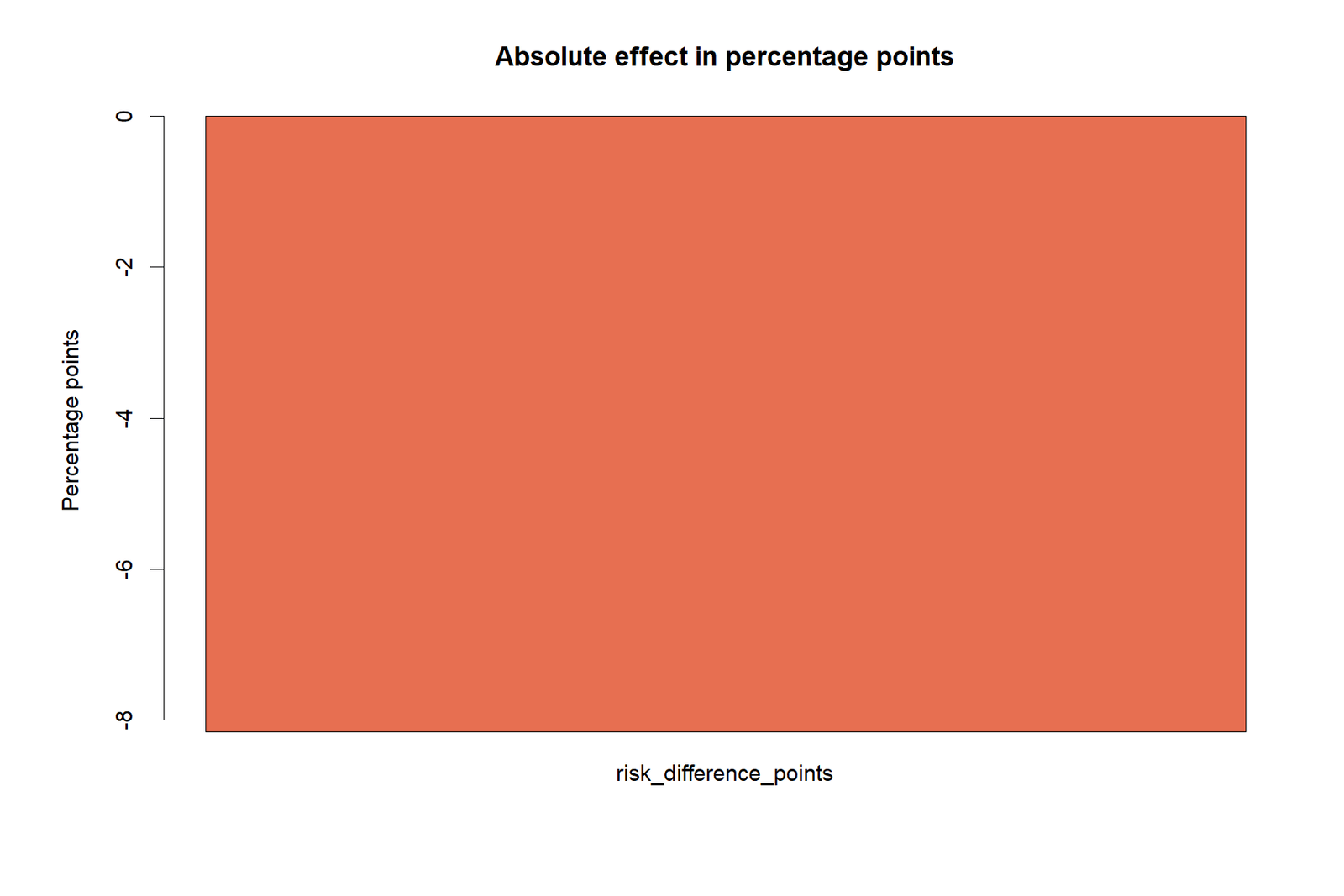
Percentage-Point Scale
The effect is displayed as −8.1589 points, an intuitive absolute scale. The compatible range is −23.6394 to +2.7080 points.
Result Summary
The compact summary aligns with Python and Excel. It should be read as an observational association with unresolved direction at the 95% level.
Risk Difference in Python, R, SPSS and Excel
Risk Difference in Python
Python can calculate the two group risks, absolute difference, Wald standard error and Wilson-based Newcombe interval transparently from four counts.
- Declare a, b, c and d explicitly.
- Calculate p1 and p0 from row totals.
- Preserve the subtraction direction.
- Use a Wilson interval function for each risk.
- Reconcile output with the workbook.
Risk Difference in R
Base R is sufficient for the point estimate and Wald interval. Wilson and Newcombe limits can be calculated directly or through validated epidemiology packages, but package defaults must be checked.
- Construct a 2 × 2 matrix with known orientation.
- Calculate proportions from row sums.
- Return probability and percentage-point units.
- Label the confidence-interval method.
- Retain the original counts in output.
Risk Difference in SPSS
SPSS CROSSTABS supplies the observed counts and row percentages. A reproducible syntax workflow can aggregate the four cells and calculate the absolute difference. The supplied SPSS PDF documents the verified analysis.
- Create G3_pass from the declared threshold.
- Request paid by G3_pass crosstabs.
- Inspect counts and row percentages.
- Calculate RD from exported or aggregated counts.
- Do not confuse a chi-square p-value with effect magnitude.
Risk Difference in Excel
The worked workbook contains Guide, Data_Input, Observed_Tables, Calculations, Diagnostics and Reporting sheets. Green cells reproduce the risk difference and verified Newcombe limits.
- Use COUNTIFS to build the four cells.
- Calculate both row risks.
- Subtract in the documented direction.
- Show Wald and Newcombe intervals separately.
- Audit every result against the reporting sheet.
Risk Difference in SAS or Stata
Procedures for binomial proportions can report risk differences directly, but defaults vary by command and may use different interval methods.
- Confirm which row is the exposed group.
- Confirm event ordering.
- Request an absolute risk contrast.
- Identify adjusted versus crude estimates.
- Name the confidence-interval method.
Adjusted Risk Difference
When confounding adjustment is required, estimate standardized predicted probabilities from an appropriate model and subtract them. A logistic regression coefficient is an adjusted log odds ratio, not an adjusted risk difference by itself.
- Fit a prespecified outcome model.
- Predict each person under both exposure levels.
- Average each prediction set.
- Subtract standardized risks.
- Use bootstrap or delta-method uncertainty.
Expandable Risk Difference Code
Python: risk difference, Wald interval and Newcombe interval
from math import sqrt
from statistics import NormalDist

a, b = 30, 9       # paid: pass, fail
c, d = 519, 91     # no paid: pass, fail
z = NormalDist().inv_cdf(0.975)

p1 = a / (a + b)
p0 = c / (c + d)
rd = p1 - p0
se = sqrt(p1*(1-p1)/(a+b) + p0*(1-p0)/(c+d))
wald = (rd - z*se, rd + z*se)

def wilson(x, n, z=1.959963984540054):
    p = x / n
    den = 1 + z*z/n
    center = (p + z*z/(2*n)) / den
    half = z*sqrt(p*(1-p)/n + z*z/(4*n*n)) / den
    return center-half, center+half

l1, u1 = wilson(a, a+b)
l0, u0 = wilson(c, c+d)
newcombe = (
    rd - sqrt((p1-l1)**2 + (u0-p0)**2),
    rd + sqrt((u1-p1)**2 + (p0-l0)**2),
)
print(p1, p0, rd, se, wald, newcombe)
R: direct point estimate and intervals
a <- 30; b <- 9
c <- 519; d <- 91
p1 <- a/(a+b)
p0 <- c/(c+d)
rd <- p1-p0
se <- sqrt(p1*(1-p1)/(a+b) + p0*(1-p0)/(c+d))
wald <- rd + c(-1,1)*qnorm(.975)*se

wilson <- function(x,n,z=qnorm(.975)) {
  p <- x/n
  den <- 1 + z^2/n
  ctr <- (p + z^2/(2*n))/den
  half <- z*sqrt(p*(1-p)/n + z^2/(4*n^2))/den
  c(ctr-half, ctr+half)
}
w1 <- wilson(a,a+b); w0 <- wilson(c,c+d)
newcombe <- c(
  rd - sqrt((p1-w1[1])^2 + (w0[2]-p0)^2),
  rd + sqrt((w1[2]-p1)^2 + (p0-w0[1])^2)
)
list(paid=p1, no_paid=p0, RD=rd, Wald=wald, Newcombe=newcombe)
SPSS: create pass variable and verify the 2 × 2 table
COMPUTE G3_pass = (G3 >= 10).
VALUE LABELS G3_pass 0 'Fail' 1 'Pass'.
EXECUTE.

CROSSTABS
  /TABLES=paid BY G3_pass
  /FORMAT=AVALUE TABLES
  /CELLS=COUNT ROW EXPECTED
  /STATISTICS=CHISQ RISK.

* Confirm paid=yes: 30 pass, 9 fail; paid=no: 519 pass, 91 fail.
* Calculate the reported RD as 30/39 - 519/610.
Excel: core formulas
Paid risk      = 30/(30+9)
No-paid risk   = 519/(519+91)
Risk difference= Paid risk - No-paid risk
Wald SE        = SQRT(PaidRisk*(1-PaidRisk)/39 + NoPaidRisk*(1-NoPaidRisk)/610)
Wald lower     = RD - 1.96*SE
Wald upper     = RD + 1.96*SE
How to Interpret and Report Risk Difference
Worked APA-Style Report
A risk-difference analysis compared the probability of passing the final grade threshold (G3 ≥ 10) between students reporting paid classes and students reporting no paid classes. The pass probability was 76.92% (30/39) in the paid-class group and 85.08% (519/610) in the no-paid-class group. The absolute risk difference was −0.0816, equivalent to −8.16 percentage points. The 95% Newcombe confidence interval ranged from −0.2364 to 0.0271 (−23.64 to +2.71 percentage points). Because the interval included zero, the data did not establish a clear absolute difference at the 95% confidence level.
Data-Discussion Paragraph
The negative point estimate was consistent with the raw G3 summaries: mean G3 was 11.21 in the paid-class group and 11.95 in the no-paid-class group, while the upper quartiles were 13 and 14. However, the paid-class group contained only 39 students and contributed 95.63% of the estimated variance. The wide interval therefore reflects limited information in the smaller group, and the observational design prevents a causal conclusion about paid instruction.
Reusable Reporting Templates
Interval Excludes Zero
Clear difference
The event risks were p1 in group 1 and p0 in group 0.
The risk difference was RD (95% CI), indicating more/fewer events per 100.
The interval excluded zero, supporting an absolute difference under the stated design assumptions.
Interval Includes Zero
Unresolved
The risk difference was RD (95% CI).
The confidence interval included zero, so the data remained compatible with a decrease, no difference or an increase within the interval limits.
Observational Interpretation
Association only
Use “the observed probability was X points lower/higher,” not “the exposure caused a change.”
Discuss group imbalance, confounding, event definition and interval width.
Required Elements in a Complete Report
- Exact group 1 and group 0 definitions.
- Event and non-event coding.
- Four 2 × 2 cell counts.
- Both group risks.
- Risk difference in probability and percentage-point units.
- Confidence-interval method and limits.
- Study-design limitations and non-causal wording.
- Supplementary ratio measures only when clearly labeled.
For broader guidance on magnitude, review effect size and confidence interval formulas.
Common Risk Difference Mistakes and Corrections
Incorrect Practice
- Subtracting groups in an unstated order.
- Calling percentage points “percent change.”
- Reporting only the point estimate.
- Using an odds ratio as though it were a risk difference.
- Ignoring group imbalance.
- Changing the event threshold after viewing results.
- Claiming causation from observational exposure.
- Using a symmetrical interval without naming the method.
Correction
- Write group 1 minus group 0 explicitly.
- Use “−8.16 percentage points.”
- Report the Newcombe interval.
- Label every scale separately.
- Show n = 39 versus n = 610.
- Prespecify G3 ≥ 10.
- Describe association and confounding.
- State whether the interval is Wald, Newcombe or another method.
Result-Specific Corrections
{tbl(['Mistaken statement','Why it is wrong','Correct statement'],[
['Paid classes lower passing by 8.16%.','Ambiguous scale and causal wording.','The observed pass probability was 8.16 percentage points lower in the paid-class group.'],
['The result proves no effect.','An interval including zero does not prove equality.','The 95% interval includes zero and also permits sizeable negative values.'],
['The paid group is 9.59% lower, therefore RD = −9.59%.','9.59% is a relative decrease, not the absolute difference.','RD = −8.16 points; RR = 0.9041.'],
['The odds ratio is 0.5845, so risk is 41.55% lower.','Odds ratio is not a risk ratio when the event is common.','Report OR separately and retain RD as the absolute measure.'],
['A larger no-paid sample will solve precision.','The paid group already drives 95.63% of variance.','Precision requires more information in the paid group.']],1100)}
Risk Difference Practice Questions
Question 1: Calculate the two risks
Using 30 passes and 9 failures in group 1, and 519 passes and 91 failures in group 0, calculate both risks.
Question 2: Calculate risk difference
Subtract group 0 from group 1.
Question 3: Interpret the sign
What does the negative sign mean when passing is the event?
Question 4: Interpret the Newcombe interval
What does −0.236394 to 0.027080 imply?
Question 5: Reverse the groups
What is the no-paid minus paid risk difference?
Question 6: Reverse the outcome
What is the paid minus no-paid failure-risk difference?
Question 7: Compare scales
Why is OR = 0.5845 not the same as RR = 0.9041?
Question 8: Diagnose imprecision
Which group contributes most to the standard error and why?
Question 9: Threshold sensitivity
At G3 ≥ 14, what is the risk difference?
Question 10: Write a responsible conclusion
Provide one sentence without causal overstatement.
Risk Difference Reports and Worked Files
Use the complete files to reproduce the counts, formulas, software output and reporting checks.
R Risk Difference ReportR calculations and paired visual results.
SPSS Risk Difference OutputSPSS tables and verified workflow output.
Worked Excel AnalysisFormula-driven input, calculations, diagnostics and reporting sheets.
Risk Difference Frequently Asked Questions
What is the risk difference formula?
Risk difference is p₁ − p₀, where each p is the event count divided by its group total.
What is absolute risk difference?
Absolute risk difference is another name for the difference between two event probabilities on the additive scale.
How do you calculate risk difference from a 2 × 2 table?
Calculate a/(a+b) for group 1, c/(c+d) for group 0, then subtract the second from the first.
Can risk difference be negative?
Yes. A negative value means the event is less common in group 1 under the stated coding.
What does a risk difference of −0.0816 mean?
It means the observed group-1 event probability is 0.0816 lower, or 8.16 percentage points lower.
Is risk difference the same as relative risk?
No. Risk difference subtracts probabilities; relative risk divides them.
What is the null value for risk difference?
Zero, because zero represents equal event probabilities.
Why use a Newcombe confidence interval?
It combines Wilson score intervals and often behaves better than a simple symmetric Wald interval for two independent proportions.
What is the worked risk difference?
Paid-class risk 0.769231 minus no-paid risk 0.850820 equals −0.081589.
What is the worked 95% confidence interval?
The Newcombe interval is −0.236394 to 0.027080.
Is the worked result statistically clear?
The 95% interval includes zero, so the direction is not resolved at that confidence level.
Why is the interval wide?
The paid-class group has only 39 observations and contributes about 95.6% of the Wald variance.
Does the result prove paid classes are harmful?
No. The exposure is observational, and self-selection or confounding may explain the association.
What is the number needed to harm?
The reciprocal of the absolute point estimate is about 12.26, but the confidence interval crosses zero, so an NNH interpretation is unstable and should not be emphasized.
Should risk difference be reported in percent or percentage points?
Percentage points are clearest for the absolute difference; relative percent change is a different measure.
Does changing the pass threshold change the result?
Yes. In the source data, the displayed risk difference ranges from about −0.44 to −18.16 points across thresholds G3 ≥ 8 through G3 ≥ 15.
Can risk difference be adjusted for confounders?
Yes, by subtracting standardized predicted risks from a suitable adjusted model.
What counts should be reported?
Report all four 2 × 2 cells, both denominators and both group risks.
What software can calculate risk difference?
Python, R, SPSS, SAS, Stata and Excel can calculate it when group and event coding are handled correctly.
What is the best one-sentence interpretation here?
The paid-class group had an observed pass probability 8.16 points lower, but the 95% interval included zero and the design does not support a causal claim.
Risk Difference Conclusion
The worked risk difference is built from a transparent 2 × 2 table: 30 passes and 9 failures among 39 students reporting paid classes, compared with 519 passes and 91 failures among 610 students reporting no paid classes. These counts produce pass risks of 76.92% and 85.08%.
The absolute difference is −0.081589, or −8.16 percentage points. The source workbook’s Newcombe 95% confidence interval is −0.236394 to 0.027080. Because zero lies inside that range, the observed negative direction is not statistically resolved at the 95% level.
The data discussion adds important context: the paid-class group contains only 39 students, supplies 95.63% of the estimated variance, has a lower mean G3, and shows negative risk differences across all displayed threshold definitions. Even so, paid classes were not randomized, and the result cannot distinguish a treatment effect from self-selection, prior difficulty or other confounding.

