Two independent proportions, one pooled-null test, and a fully audited 649-student example

Z Test for Proportions: Formula, Example, Interpretation, Python, R, SPSS, SAS and Excel Guide

The Z Test for Proportions compares one or two population proportions with a standard-normal test statistic. This worked analysis compares male and female G3 pass proportions at the G3 ≥ 10 threshold, explains why the hypothesis test pools the proportions while the confidence interval does not, and traces every count, standard error, residual, chart and software result back to the 649 student records.

649 valid students216/266 male passes333/383 female passesz = −1.9927p = 0.04629

Z Test for Proportions Model Overview

The Z Test for Proportions evaluates whether an observed sample proportion differs from a hypothesised population value or whether two independent sample proportions differ more than sampling variation would reasonably explain. The present analysis is a two-sample Z Test for Proportions: males and females are independent groups, the binary response is whether the final grade G3 is at least 10, and the null hypothesis states that the two population pass proportions are equal.

The data contain 266 male students and 383 female students. Exactly 216 males and 333 females passed. Therefore, the observed male pass proportion is 0.8120 and the female pass proportion is 0.8695. The raw difference, defined as male minus female, is −0.05742. On the percentage-point scale, males had a pass rate 5.74 points lower than females.

The Exact Research Question

Do male and female students have the same population probability of achieving G3 ≥ 10, or is the observed 5.74-percentage-point difference large enough to reject equality?

H₀: p_M − p_F = 0

H₁: p_M − p_F ≠ 0

Why Two Standard Errors Appear

The central technical distinction is not optional. Under the equality null, both groups are assumed to share one common proportion, so the test statistic uses the pooled proportion 0.845917 and pooled null standard error 0.028815. A confidence interval estimates the actual difference without imposing equality, so it uses the unpooled standard error 0.029499. Mixing these two standard errors is one of the most common errors in a two-proportion Z test.

Worked-result preview: z = −1.992745 and two-sided p = 0.046289. At α = .05, the pooled-null Z Test for Proportions rejects equal pass proportions. The direction is lower for males because the analysis subtracts female proportion from male proportion.

Precision warning: the unpooled Wald 95% interval for the difference is approximately −11.52 to +0.04 percentage points and narrowly includes zero. This does not invalidate the test result; it reflects the use of different standard errors for the pooled null test and the unpooled interval, plus the borderline nature of the evidence.

AdvertisementGoogle AdSense top placement reserved here

Quick Answer: Z Test for Proportions Result

The two-sample Z Test for Proportions compares 216 passes among 266 males with 333 passes among 383 females. The difference is negative, the test statistic falls just beyond the conventional two-sided 5% boundary, and the result is statistically significant but close to the threshold.

Male pass proportion81.20%

Female pass proportion86.95%

Male − female−5.74 pp

Two-sided p-value0.04629

Statistical Decision

Procedure: two-sample pooled Z Test for Proportions
Test statistic: z = −1.992745
Two-sided p: 0.046289
Decision at α = .05: reject H₀
Decision at α = .01: do not reject H₀

Data Meaning

Male passes: 216 of 266.
Female passes: 333 of 383.
Both groups contain exactly 50 failures.
The unequal denominators create different failure rates: 18.80% versus 13.05%.
The evidence is statistically detectable but small in standardized magnitude.

Plain-language conclusion: in these data, female students passed at a higher rate than male students. The pooled two-sided Z Test for Proportions gives just enough evidence at the .05 level to reject equal population pass proportions, but the result should be described as borderline rather than overwhelming.

The same 2 × 2 data can also be described with relative risk, an odds ratio, or the equivalent uncorrected Pearson chi-square test. Those measures answer related but not identical questions.

What Is a Z Test for Proportions?

A Z Test for Proportions converts a difference involving proportions into a standard-normal score. The numerator contains the observed departure from the null hypothesis. The denominator contains the standard error expected under that null. The resulting z value states how many null-standard-error units the observed result lies from the hypothesised value.

One-Sample and Two-Sample Forms

One-proportion Z test

Compares one sample proportion with a fixed null value p₀.

Two-proportion Z test

Compares independent sample proportions p̂₁ and p̂₂.

Two-sided test

Tests whether the difference is nonzero in either direction.

One-sided test

Tests a prespecified direction such as p_M < p_F.

What Is Being Standardized?

The present numerator is 0.812030 − 0.869452 = −0.057422. Under H₀, the pooled estimate of the common pass proportion is 549/649 = 0.845917. The null predicts a standard deviation of 0.028815 for the difference between the two sample proportions. Dividing −0.057422 by 0.028815 produces z = −1.992745.

Interpretation of sign: the negative sign follows only from the subtraction order. If female minus male were used, z would be +1.992745 and the two-sided p-value would remain 0.046289.

What the Test Does Not Prove

A statistically significant Z Test for Proportions does not prove that gender causes the difference, that every male has lower performance than every female, or that the result generalises beyond the sampling process. The procedure evaluates an association between group membership and a binary outcome. Design quality, selection, confounding and measurement still govern causal and population claims. Review sampling methods and sampling bias before extending the result.

Research Question, Hypotheses and Data Design

Group 1Male students, n = 266

Group 2Female students, n = 383

Binary outcomePass = G3 ≥ 10

Research Question

Is the population pass proportion for male students different from the population pass proportion for female students?

Component	Mathematical statement	Meaning
Null hypothesis	H₀: p_M = p_F	Male and female population pass probabilities are equal.
Two-sided alternative	H₁: p_M ≠ p_F	The population pass probabilities differ in either direction.
Directional alternative	H₁: p_M < p_F	Male pass probability is lower; this must be prespecified.
Observed estimate	p̂_M − p̂_F = −0.057422	The sample difference is −5.74 percentage points.

Why the Direction Must Be Declared Before Testing

The one-sided p-value for the prespecified male-lower alternative is 0.023145. It is exactly half the two-sided p-value because the z statistic points in the predicted direction. Selecting that alternative only after seeing the data would artificially improve the apparent evidence. The public report therefore uses the safer two-sided test unless a directional hypothesis was established in advance.

Methods statement: “A two-sided two-sample Z Test for Proportions compared the proportion of male and female students with G3 ≥ 10. The null test used the pooled proportion, and confidence intervals used group-specific or unpooled standard errors.”

When to Use the Z Test for Proportions

Use It When

The outcome is binary for every observation.
The groups are independent rather than paired.
Each observation belongs to only one group.
Success and failure counts are sufficiently large.
The sampling or assignment mechanism supports independence.
The goal is inference about one proportion or a difference between two proportions.
The hypotheses and direction are defined before examining the result.

Choose Another Method When

The same people are measured twice; use McNemar’s test for paired binary data.
Expected counts are small; consider Fisher’s exact test or another exact method.
The outcome has more than two categories without a justified binary cut point.
Multiple predictors or confounders require adjustment; use logistic regression.
Survey weights, clusters or repeated measures require design-based standard errors.
The groups are not independent because students are nested in classes or schools.

Decision Flow

Step 1Is the outcome binary?

Code one clearly defined success and one failure.

→

Step 2Are groups independent?

If paired, do not use the independent two-proportion formula.

→

Step 3Are counts large enough?

Check expected successes and failures under the null.

The Z Test for Proportions is an asymptotic method. “Large enough” is not a purely ceremonial condition: the standard-normal approximation depends on the binomial distribution being well represented by a normal distribution. In this example, all null-expected counts exceed 40, so the approximation is strong.

Z Test for Proportions Variants and Their Meanings

The keyword “Z Test for Proportions” covers several procedures. Selecting the right form depends on the number of samples, the null hypothesis, group dependence and whether the analysis is testing or estimating.

Variant	Null structure	Standard error	Typical use
One-sample Z test	p = p₀	Uses p₀ under H₀	Compare one observed rate with a benchmark.
Two-sample pooled Z test	p₁ = p₂	Uses pooled p̂ under H₀	Primary test in this article.
Difference confidence interval	Estimate p₁ − p₂	Uses unpooled group proportions	Quantify the plausible difference.
Paired proportions test	Marginal probabilities equal	Uses discordant pairs	Use McNemar’s test, not the independent formula.
Exact two-sample test	No large-sample approximation	Conditional or unconditional exact probability	Useful with sparse counts.

Pooled Does Not Mean the Groups Are Permanently Combined

Pooling occurs only inside the null standard error because H₀ says the two population proportions are the same. It does not erase the male and female labels, and it is not used to estimate the final difference. The observed difference remains −0.057422 throughout.

Continuity Correction

Some chi-square or proportion-testing software applies a continuity correction by default. That correction generally produces a larger p-value than the uncorrected Z Test for Proportions. This post reports the uncorrected pooled z statistic because it matches the workbook, Python, R and SPSS reference values. Software settings must be stated when results are close to .05.

Correction and Method Sensitivity

Method choice	Typical effect	Reporting requirement
Uncorrected pooled z	Primary result: p = 0.046289	State that no continuity correction was used.
Continuity-corrected chi-square	Usually increases p near the boundary	Name the correction if software applies it.
Fisher exact test	Uses an exact conditional probability	Use for sparse counts or as a sensitivity check.
Newcombe difference interval	Wider score-based interval	Name the interval method rather than writing only “95% CI.”

Borderline-result safeguard: when p is near .05, report the exact p-value, the selected correction setting, confidence intervals and effect size. A binary “significant/not significant” label discards important information.

Variables, Coding and Data Dictionary

Variable	Role	Coding	Valid N	Meaning
sex	Independent grouping variable	M = male; F = female	649	Defines the two independent groups.
G3	Original quantitative outcome	Final grade from 0 to 19	649	Source variable before dichotomisation.
G3 pass	Binary response	1 if G3 ≥ 10; 0 if G3 < 10	649	Success variable used by the Z Test for Proportions.
group order	Direction convention	Male minus female	649	Determines the negative sign of the difference and z.

Sample Composition

Group	Pass	Fail	Total	Sample share
Male	216	50	266	40.99%
Female	333	50	383	59.01%
Total	549	100	649	100.00%

Why the Equal Failure Counts Do Not Mean Equal Failure Rates

Both groups contain 50 failures, but their denominators differ. The male failure proportion is 50/266 = 18.80%, whereas the female failure proportion is 50/383 = 13.05%. Proportion inference always uses the numerator together with its denominator. Comparing counts alone would conceal the actual rate difference.

Binary coding rule

G3 pass = 1 when G3 >= 10; otherwise 0

The threshold must be declared and applied identically to both groups.

Subtraction order

Difference = male proportion − female proportion.

Reversing order changes the sign, not the two-sided evidence.

Transparent coding allows the reader to reconstruct the table from the raw data. See frequency and relative-frequency tables and two-way tables and relative frequencies for the descriptive foundation.

Z Test for Proportions Formula and Manual Calculation

The manual calculation follows seven steps. Each stage is shown because most Z Test for Proportions errors arise from a wrong denominator, reversed coding, or use of the unpooled standard error inside the null test.

Notation Used in the Two-Proportion Formula

Symbol	Definition	Worked value
x_M	Male successes	216
n_M	Male sample size	266
x_F	Female successes	333
n_F	Female sample size	383
p̂_M, p̂_F	Observed group proportions	0.812030 and 0.869452
p̂_pool	Common null proportion	0.845917
SE₀	Pooled null standard error	0.0288153
SE_diff	Unpooled estimation standard error	0.0294989

Step 1: Compute the Group Proportions

p̂_M = 216/266 = 0.812030

p̂_F = 333/383 = 0.869452

Step 2: Compute the Observed Difference

p̂_M − p̂_F = 0.812030 − 0.869452 = −0.057422

The point estimate equals −5.742 percentage points. This is the substantive effect on the absolute scale.

Step 3: Pool the Proportions Under H₀

p̂_pool = (216 + 333)/(266 + 383) = 549/649 = 0.845917

Null Allocation by Group

Group	Null pass probability	Expected passes	Expected failures
Male	0.845917	225.014	40.986
Female	0.845917	323.986	59.014

Step 4: Compute the Pooled Null Standard Error

SE₀ = √[p̂_pool(1−p̂_pool)(1/266 + 1/383)] = 0.0288153

Step 5: Compute the Z Statistic

z = (−0.0574216 − 0)/0.0288153 = −1.9927455

Step 6: Convert Z to a Probability

p = 2P(Z ≤ −|−1.9927455|) = 0.0462893

The corresponding one-sided probability for the prespecified alternative p_M < p_F is 0.0231447.

Step 7: Build a Difference Confidence Interval

SE_diff = √[p̂_M(1−p̂_M)/266 + p̂_F(1−p̂_F)/383] = 0.0294989

95% Wald CI = −0.0574216 ± 1.96(0.0294989) = [−0.115239, 0.000396]

Calculation audit: the workbook-calculated and independently verified values are identical to displayed precision: z = −1.9927454994 and p = 0.0462893224.

Observed Tables, Expected Counts and Raw-Data Profiles

Observed 2 × 2 Table

Group	Pass (G3 ≥ 10)	Fail (G3 < 10)	Total	Pass proportion
Male	216	50	266	81.203%
Female	333	50	383	86.945%
Total	549	100	649	84.592%

Expected Counts Under Equal Proportions

Group	Expected pass	Expected fail	Observed − expected pass	Adjusted residual for pass
Male	225.014	40.986	−9.014	−1.9927
Female	323.986	59.014	+9.014	+1.9927

The male group contains about nine fewer passes than the equality null predicts, and the female group contains about nine more. The adjusted residuals equal ±1.9927 in a 2 × 2 table, which is the same standardized signal as the two-proportion z statistic.

Group-Specific Proportion Intervals

Group	Observed proportion	Wald 95% CI	Wilson 95% CI	Interval width (Wilson)
Male	0.812030	0.765080 to 0.858980	0.760761 to 0.854415	0.093654
Female	0.869452	0.835711 to 0.903193	0.832009 to 0.899556	0.067547

The male interval is wider because the male sample is smaller. The overlap between separate group intervals is not itself the formal two-sample test. The difference must be standardized directly.

Raw G3 Score Distribution by Gender

G3 score	Male count	Male %	Female count	Female %
0	8	3.01%	7	1.83%
1	1	0.38%	0	0.00%
5	1	0.38%	0	0.00%
6	3	1.13%	0	0.00%
7	3	1.13%	7	1.83%
8	15	5.64%	20	5.22%
9	19	7.14%	16	4.18%
10	45	16.92%	52	13.58%
11	50	18.80%	54	14.10%
12	28	10.53%	44	11.49%
13	28	10.53%	54	14.10%
14	22	8.27%	41	10.70%
15	17	6.39%	32	8.36%
16	13	4.89%	23	6.01%
17	8	3.01%	21	5.48%
18	4	1.50%	11	2.87%
19	1	0.38%	1	0.26%

The binary pass variable is created from a richer 0–19 distribution. Female scores have a mean of 12.253 and median of 12, compared with a male mean of 11.406 and median of 11. The Z Test for Proportions intentionally ignores distances above and below the cut point; it answers only whether the probability of reaching the threshold differs.

Original G3 Descriptive Statistics

Group	N	Mean	Median	Sample SD	Q1	Q3	Range
Male	266	11.406	11	3.321	10	13	0–19
Female	383	12.253	12	3.124	10	14	0–19

Threshold Sensitivity

Pass threshold	Male successes	Male %	Female successes	Female %	Difference (pp)	z	Two-sided p
G3 ≥ 8	250	93.98%	369	96.34%	-2.36	-1.4080	0.159100
G3 ≥ 9	235	88.35%	349	91.12%	-2.78	-1.1589	0.246500
G3 ≥ 10	216	81.20%	333	86.95%	-5.74	-1.9927	0.046300
G3 ≥ 11	171	64.29%	281	73.37%	-9.08	-2.4749	0.013300
G3 ≥ 12	121	45.49%	227	59.27%	-13.78	-3.4621	0.000536
G3 ≥ 13	93	34.96%	183	47.78%	-12.82	-3.2485	0.001160
G3 ≥ 14	65	24.44%	129	33.68%	-9.25	-2.5303	0.011400
G3 ≥ 15	43	16.17%	88	22.98%	-6.81	-2.1261	0.033500

The G3 ≥ 10 result is not the only point at which the distributions differ. At stricter thresholds from 11 through 15, the female proportion remains higher and the z statistics are significant. The largest absolute gap occurs at G3 ≥ 12: 45.49% for males versus 59.27% for females, a difference of −13.78 percentage points. This sensitivity analysis is descriptive and should not replace a prespecified primary threshold.

Threshold Pattern Summary

Threshold range	Direction	Statistical pattern	Data implication
G3 ≥ 8 to 9	Female higher	Not significant at .05	The very-low threshold leaves little room for group separation.
G3 ≥ 10	Female higher	Borderline, p = .0463	Primary pass threshold.
G3 ≥ 11 to 15	Female higher	All significant at .05	The gap persists and is larger at stricter standards.
Maximum gap at G3 ≥ 12	Female higher by 13.78 pp	p = 0.000536	Separation is strongest around the middle-upper distribution.

Complete Z Test for Proportions Results

Observed difference−0.057422

Male minus female

Pooled proportion0.845917

Null estimate

Pooled null SE0.028815

Used for z

Z statistic−1.992745

Standard-normal units

Two-sided p0.046289

Uncorrected test

Phi effect size0.0782

Small standardized association

Primary Result Table

Test	Difference	Pooled SE	z	Two-sided p	Decision at .05
Two-sample Z Test for Proportions	−0.0574216	0.0288153	−1.9927455	0.0462893	Reject H₀

Inference on Multiple Scales

Measure	Estimate	No-effect value	Interpretation
Risk difference (M − F)	−0.057422	0	Male pass probability is 5.74 percentage points lower.
Relative risk (M/F)	0.933957	1	Male pass probability is about 93.40% of the female probability.
Odds ratio	0.648649	1	Male pass odds are about 35.14% lower.
Pearson χ² equivalent	3.971035	0	Equals z² for the uncorrected 2 × 2 test.
Phi coefficient	0.078222	0	Small standardized association.

Confidence-Interval Comparison

Interval	Lower	Upper	Contains zero?	Purpose
Unpooled Wald difference	−0.115239	+0.000396	Yes, narrowly	Workbook difference interval.
Newcombe score difference	−0.138795	+0.022405	Yes	More conservative supplementary score interval.
Male Wald proportion	0.765080	0.858980	Not applicable	Group-specific descriptive uncertainty.
Female Wald proportion	0.835711	0.903193	Not applicable	Group-specific descriptive uncertainty.

Unpooled Variance Contributions

Group	p̂(1−p̂)/n	Share of unpooled variance	Interpretation
Male	0.00057410	65.98%	Smaller n and lower p produce the larger contribution.
Female	0.00029609	34.02%	Larger n narrows the female component.
Total	0.00087019	100.00%	Square root = 0.0294989.

Why the P-Value and Wald Interval Straddle the .05 Boundary Differently

The hypothesis test uses the pooled null standard error 0.028815, while the Wald difference interval uses the slightly larger unpooled standard error 0.029499. The unpooled value is 2.37% larger. Because the result is very close to the threshold, that small standard-error difference is enough for p = .0463 while the unpooled interval reaches +0.0004. This is a legitimate mathematical consequence, not a spreadsheet inconsistency.

Lower-tail probability0.023145

Relevant to p_M < p_F.

Upper-tail probability0.976855

Relevant to p_M > p_F.

Two-sided probability0.046289

Primary public result.

Interpretation: the uncorrected pooled Z Test for Proportions finds a statistically detectable difference at α = .05, z = −1.99, p = .046. The female pass proportion is higher, but the evidence is borderline and the standardized association is small.

AdvertisementGoogle AdSense placement reserved after the Results section

Z Test for Proportions Assumptions and Diagnostic Checks

The reliability of a Z Test for Proportions depends on design and approximation conditions. The numerical success-failure check is excellent here, but that does not automatically establish random sampling or causal interpretation.

Binary response

Every student is coded pass or fail using G3 ≥ 10.

Independent groups

Each student belongs to one gender group and appears once.

Independent observations

No repeated record is used in the two-group table.

Large expected counts

All pooled-null expected cells are above 40.

Transparent threshold

The G3 ≥ 10 rule is stated before interpretation.

Representative mechanism

Population generalisation still requires defensible sampling.

Success-Failure Condition Audit

Group	Observed successes	Observed failures	Null-expected successes	Null-expected failures	Condition
Male	216	50	225.014	40.986	Strong
Female	333	50	323.986	59.014	Strong

Observed-to-Expected Deviations

Cell	Observed	Expected	Difference	Direction
Male pass	216	225.014	−9.014	Fewer than expected under equality
Male fail	50	40.986	+9.014	More than expected
Female pass	333	323.986	+9.014	More than expected
Female fail	50	59.014	−9.014	Fewer than expected

Independence Is a Design Condition

The spreadsheet cannot prove that observations are independent. If students share classrooms, teachers or schools, the effective information may be lower than 649 independent records. Cluster-robust or multilevel methods may be needed when the sampling unit differs from the student unit.

Effect of Dichotomising G3

Turning a 0–19 score into pass/fail simplifies interpretation but discards distance information. A student scoring 10 and a student scoring 19 are both successes, while scores 9 and 0 are both failures. The threshold sensitivity table and raw distribution are therefore important companions to the primary Z Test for Proportions.

Do not confuse sample size with design quality: large counts improve the normal approximation, but they cannot repair biased sampling, misclassification, dependence or post-hoc threshold selection.

Z Test for Proportions Versus Related Tests

The Z Test for Proportions belongs to a family of methods for 2 × 2 and binary-outcome data. The appropriate companion or alternative depends on whether the goal is testing, effect estimation, exact inference, adjustment or paired analysis.

Method	Primary output	Relationship to this analysis	When preferable
Two-proportion z test	z and p-value	Primary method; uncorrected z² = Pearson χ².	Large independent samples and direct proportion comparison.
Pearson chi-square	χ² and p-value	Gives χ² = 3.9710 and the same p without correction.	General contingency-table framing.
Fisher’s exact test	Exact conditional p-value	Avoids the normal approximation.	Small or sparse cell counts.
Relative risk	Ratio of probabilities	RR = 0.9340 describes magnitude.	When a risk ratio is substantively meaningful.
Odds ratio	Ratio of odds	OR = 0.6486 describes odds, not probabilities.	Case-control or logistic-model contexts.
McNemar’s test	Discordant-pair test	Not appropriate here because groups are independent.	Before/after or matched binary observations.
Logistic regression	Adjusted odds effects	Can add school, age and other covariates.	Confounding adjustment and prediction.

Equivalence with the Pearson 2 × 2 Test

z² = (−1.9927455)² = 3.9710346

The uncorrected Pearson chi-square statistic for the same 2 × 2 table is 3.9710346 with one degree of freedom. The p-values match because a one-degree-of-freedom chi-square variable is the square of a standard-normal variable.

Why Relative Risk and Odds Ratio Do Not Replace the Z Test

The relative risk and odds ratio quantify effect size on ratio scales, while the Z Test for Proportions provides a null-hypothesis test on the absolute difference. A complete report can include all three, but it should not treat them as interchangeable. The relative risk guide and odds ratio guide explain those scales in detail.

Z Test for Proportions Calculator: Step-by-Step Workflow

A two-proportion Z test calculator needs only four counts, but the user must define which row is group 1, which outcome is success and whether the alternative is two-sided or directional.

Male successes216

Male total266

Female successes333

Female total383

Calculator Workflow

Step	Calculation	Worked value	Check
1	p̂_M = x_M/n_M	216/266 = 0.812030	0 ≤ p̂ ≤ 1
2	p̂_F = x_F/n_F	333/383 = 0.869452	0 ≤ p̂ ≤ 1
3	Difference = p̂_M − p̂_F	−0.057422	Direction matches group order
4	Pool successes and totals	549/649 = 0.845917	Use only for H₀
5	Compute pooled SE	0.0288153	Positive and plausible
6	Compute z	−1.9927455	Difference divided by SE
7	Compute two-sided p	0.0462893	Double the smaller tail
8	Compute unpooled interval SE	0.0294989	Do not pool for estimation

Result Verification Checklist

Counts reconcile216 + 50 = 266 and 333 + 50 = 383.

Grand totals reconcile549 + 100 = 649.

Sign is correctMale − female is negative.

Null SE is pooledUses 549/649.

Interval SE is unpooledUses both group estimates separately.

Tail choice is statedPrimary result is two-sided.

For broader calculation rules, see the two-proportion z-test guide, p-value, significance level and test statistic, and confidence-interval formula.

Python Z Test for Proportions Chart Interpretations

Each Python figure supports a separate stage of the data analysis. The charts move from raw counts to proportions, uncertainty, standard-error logic and the final inferential decision.

1Observed 2 × 2 Table

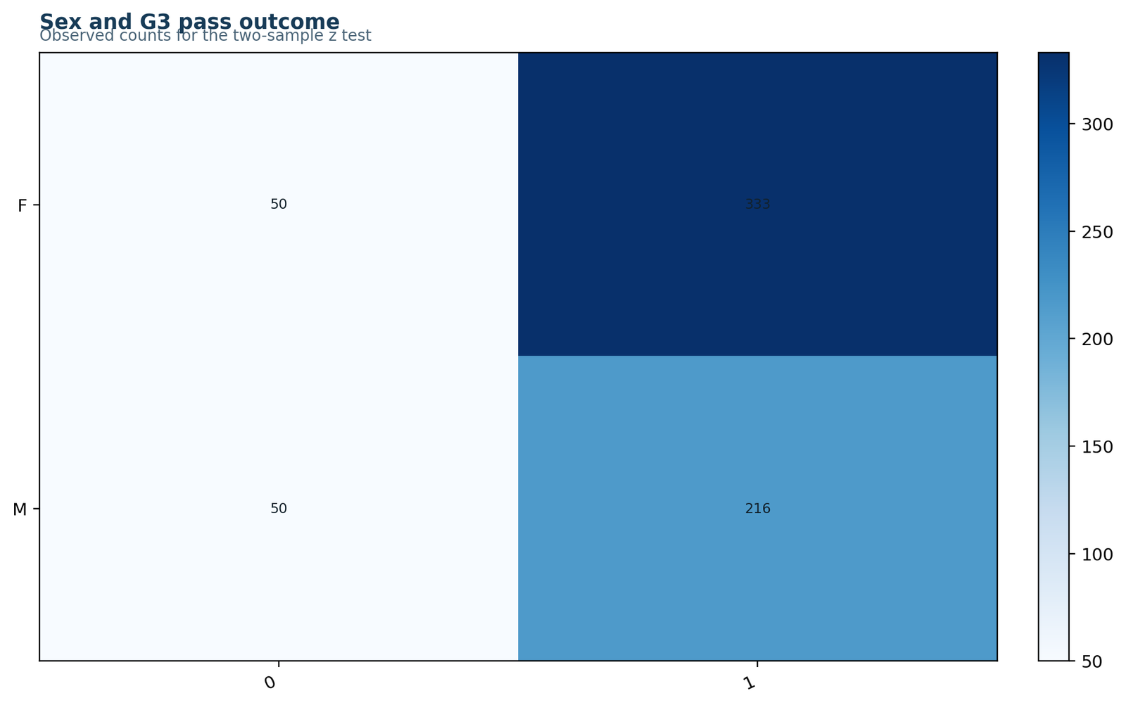
Python Observed 2 × 2 Table for the Z Test for Proportions — Python figure 1. Observed 2 × 2 Table for the male-versus-female G3 pass analysis.

Exact data reading

The table contains 216 male passes and 50 male failures, compared with 333 female passes and 50 female failures. Equal failure counts are visually striking, but the denominators differ by 117 students. The inferential comparison must therefore use proportions rather than raw counts.

Analytical meaning

The chart is interpreted on the scale it displays and reconciled with the workbook values.

Next step: Verify that every row and column total reconciles before calculating a z statistic.

2Male and Female Pass Proportions

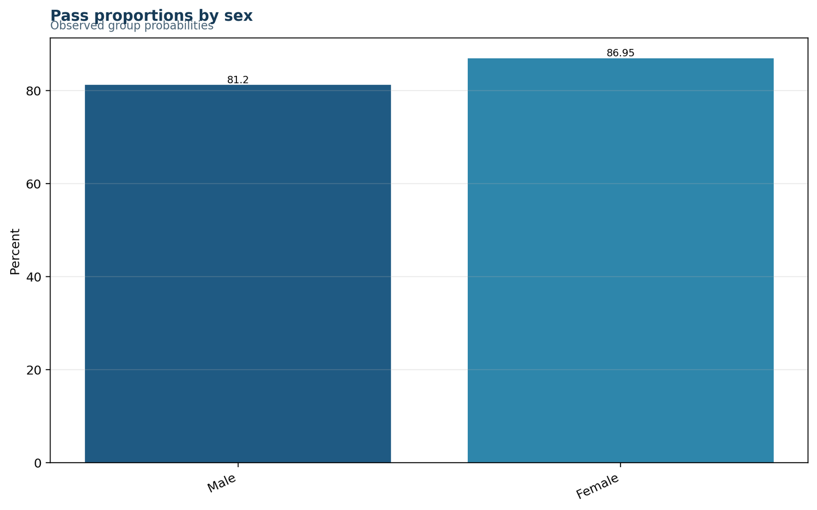
Python Male and Female Pass Proportions for the Z Test for Proportions — Python figure 2. Male and Female Pass Proportions for the male-versus-female G3 pass analysis.

Exact data reading

The bars show 81.20% for males and 86.95% for females. The vertical separation is 5.74 percentage points. Because the male bar is lower, male-minus-female produces a negative difference and negative z.

Analytical meaning

The chart is interpreted on the scale it displays and reconciled with the workbook values.

Next step: Read the absolute gap first; statistical significance does not communicate effect size by itself.

3Group-Specific 95% Intervals

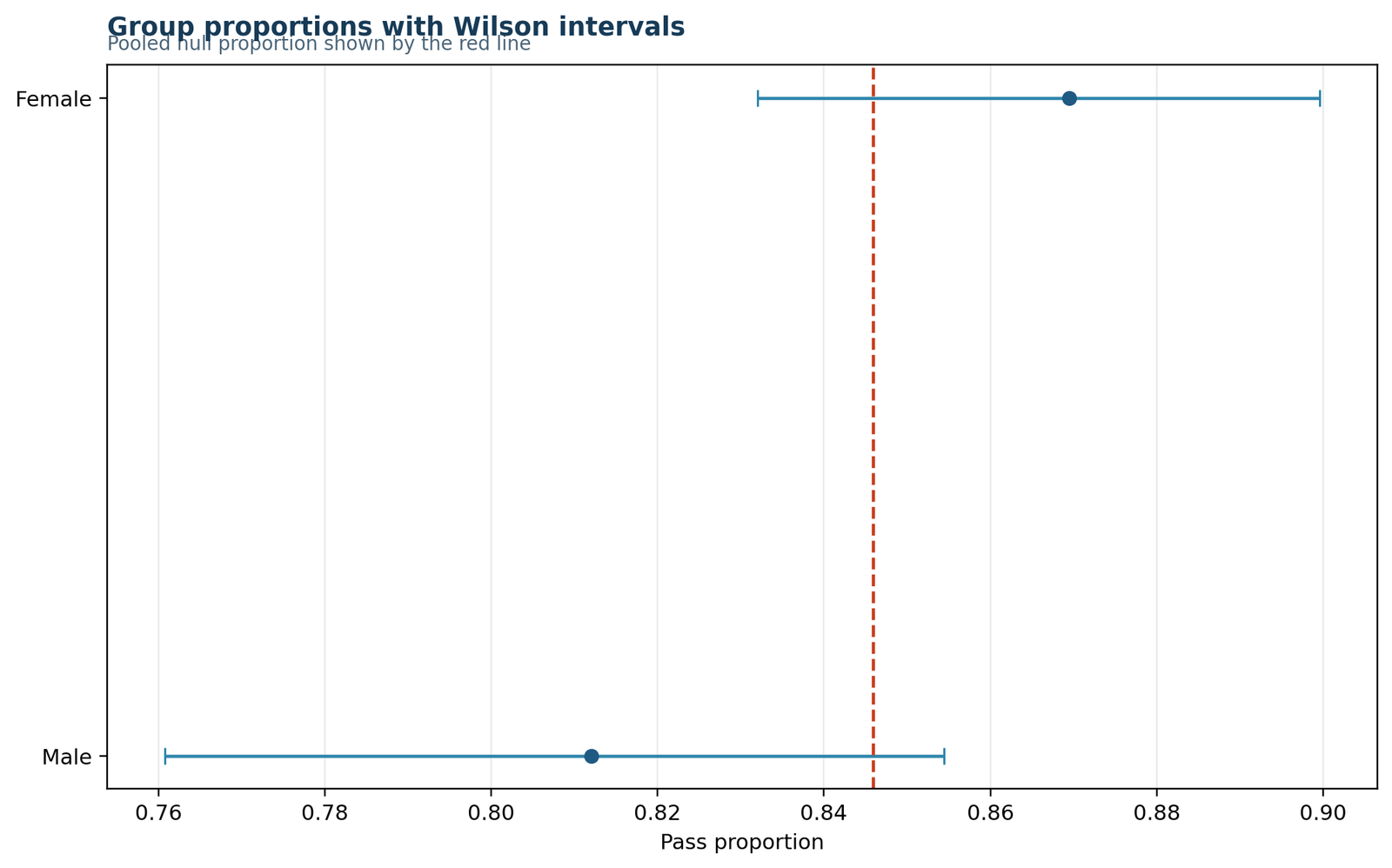
Python Group-Specific 95% Intervals for the Z Test for Proportions — Python figure 3. Group-Specific 95% Intervals for the male-versus-female G3 pass analysis.

Exact data reading

The male Wald interval is 76.51%–85.90%, while the female interval is 83.57%–90.32%. The male interval is wider because n = 266 is smaller than n = 383. Overlap does not replace the formal test of the difference.

Analytical meaning

The chart is interpreted on the scale it displays and reconciled with the workbook values.

Next step: Use a direct difference interval or two-sample test rather than judging significance by visual overlap alone.

4Pooled and Unpooled Standard Errors

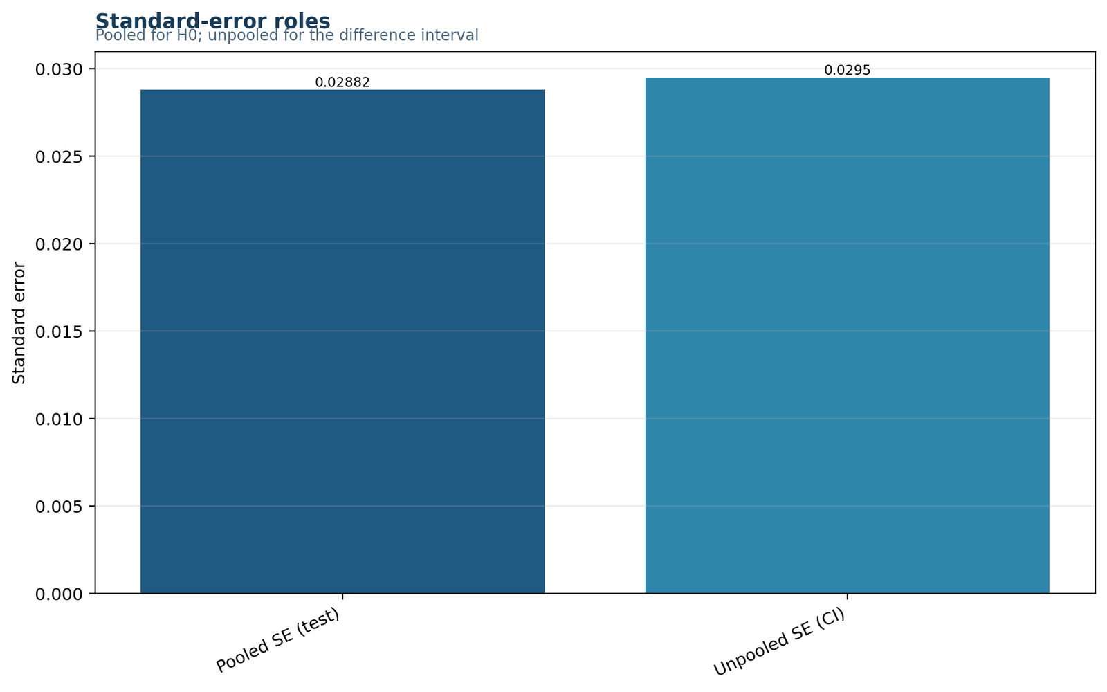
Python Pooled and Unpooled Standard Errors for the Z Test for Proportions — Python figure 4. Pooled and Unpooled Standard Errors for the male-versus-female G3 pass analysis.

Exact data reading

The pooled null SE is 0.028815 and the unpooled interval SE is 0.029499. Their difference is small in absolute terms but consequential because the result lies close to .05.

Analytical meaning

The chart is interpreted on the scale it displays and reconciled with the workbook values.

Next step: Match the standard error to the task: pooled for testing equality, unpooled for estimating the difference.

5Z Test Result Summary

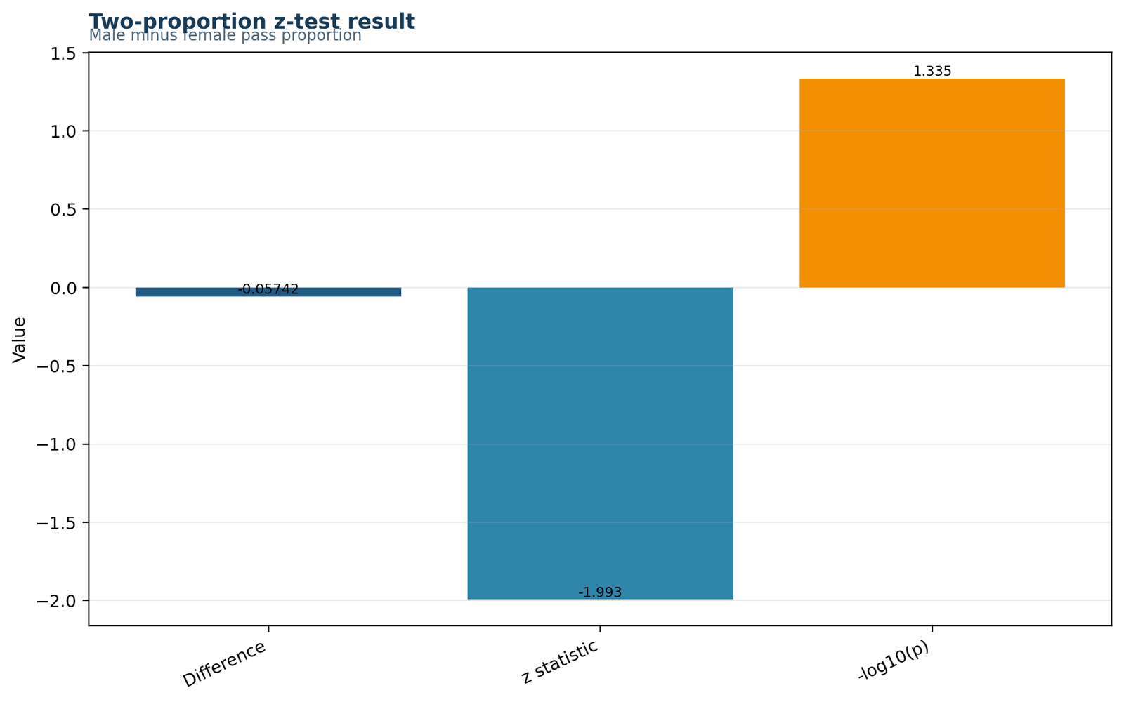
Python Z Test Result Summary for the Z Test for Proportions — Python figure 5. Z Test Result Summary for the male-versus-female G3 pass analysis.

Exact data reading

The summary places z = −1.9927 with p = .04629 beside the 5.74-point gap. The result crosses the .05 threshold but not the .01 threshold, and phi = .078 indicates a small standardized association.

Analytical meaning

The chart is interpreted on the scale it displays and reconciled with the workbook values.

Next step: Report the exact p-value and effect size; avoid describing the evidence as strong or decisive.

AdvertisementGoogle AdSense placement reserved after the Python figures

R Z Test for Proportions Charts in Paired Rows

The R figures reproduce the data and test from a second software environment. The paired layout keeps related displays together: counts with proportions, intervals with standard errors, and the z reference with the final summary.

Cross-software reconciliation: R, Python, Excel and SPSS use the same four counts and reproduce z = −1.9927455 and p = 0.0462893 when the uncorrected pooled test is requested.

R figure pair 1: Observed 2 × 2 Table and Male and Female Pass Proportions

R Observed 2 × 2 Table for the Z Test for Proportions — R figure 1. Observed 2 × 2 Table.

R Male and Female Pass Proportions for the Z Test for Proportions — R figure 2. Male and Female Pass Proportions.

First figure

Observed 2 × 2 Table

The observed table confirms that both groups contain 50 failures, while female successes exceed male successes because the female group is larger.

Check: values agree with the workbook and Python output.

Second figure

Male and Female Pass Proportions

The proportion plot converts the counts to 81.20% and 86.95%, revealing the 5.74-point rate gap.

Check: direction remains male minus female throughout.

R figure pair 2: Group-Specific 95% Intervals and Pooled and Unpooled Standard Errors

R Group-Specific 95% Intervals for the Z Test for Proportions — R figure 3. Group-Specific 95% Intervals.

R Pooled and Unpooled Standard Errors for the Z Test for Proportions — R figure 4. Pooled and Unpooled Standard Errors.

First figure

Group-Specific 95% Intervals

The interval figure shows greater uncertainty for males and places the point estimates in their group-specific sampling ranges.

Check: values agree with the workbook and Python output.

Second figure

Pooled and Unpooled Standard Errors

The standard-error display distinguishes 0.028815 for the pooled null test from 0.029499 for the unpooled interval.

Check: direction remains male minus female throughout.

R figure pair 3: Standard-Normal Reference and Z Test Result Summary

R Standard-Normal Reference for the Z Test for Proportions — R figure 5. Standard-Normal Reference.

R Z Test Result Summary for the Z Test for Proportions — R figure 6. Z Test Result Summary.

First figure

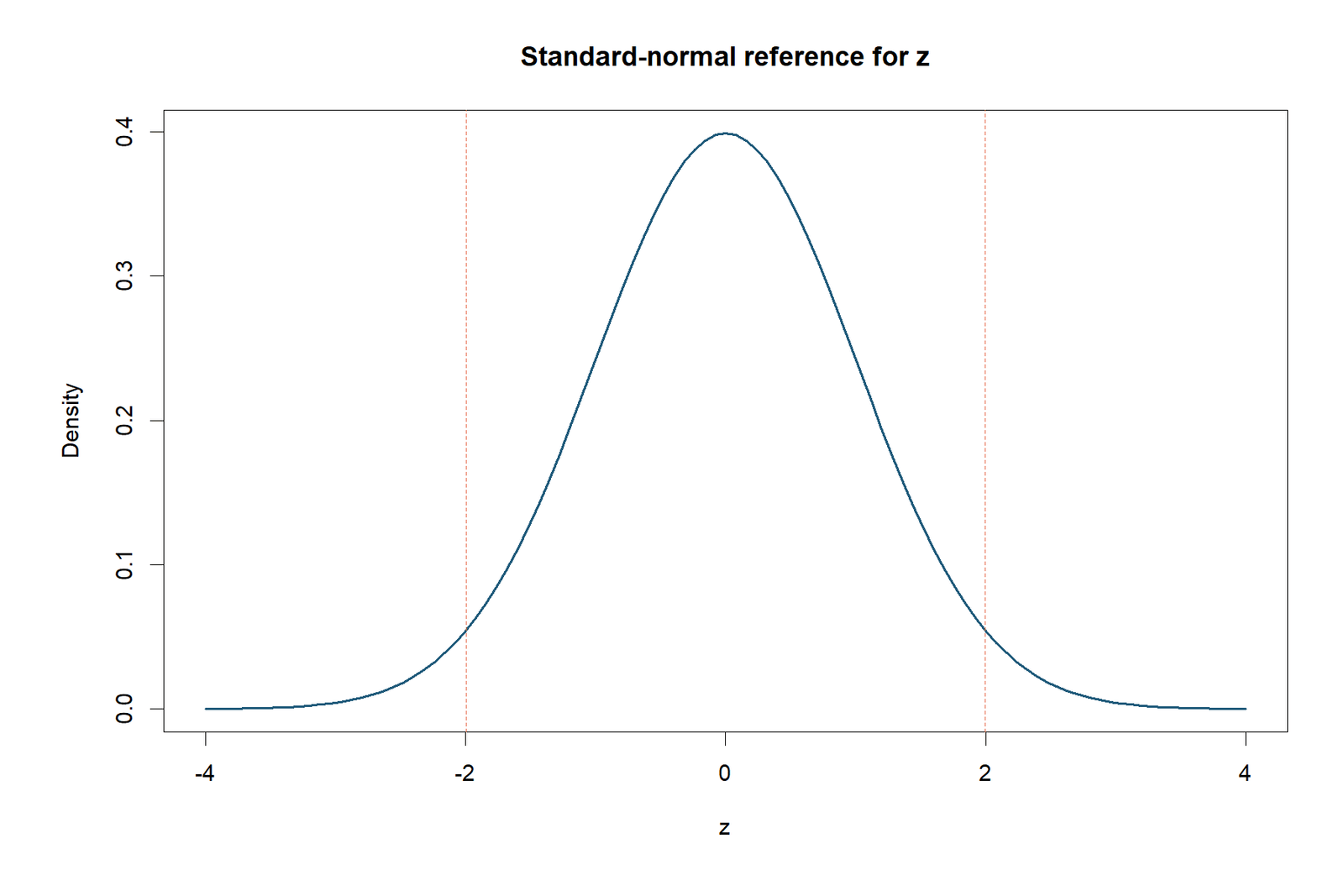
Standard-Normal Reference

The standard-normal reference places −1.9927 in the lower tail and mirrors the equal upper-tail area used in the two-sided p-value.

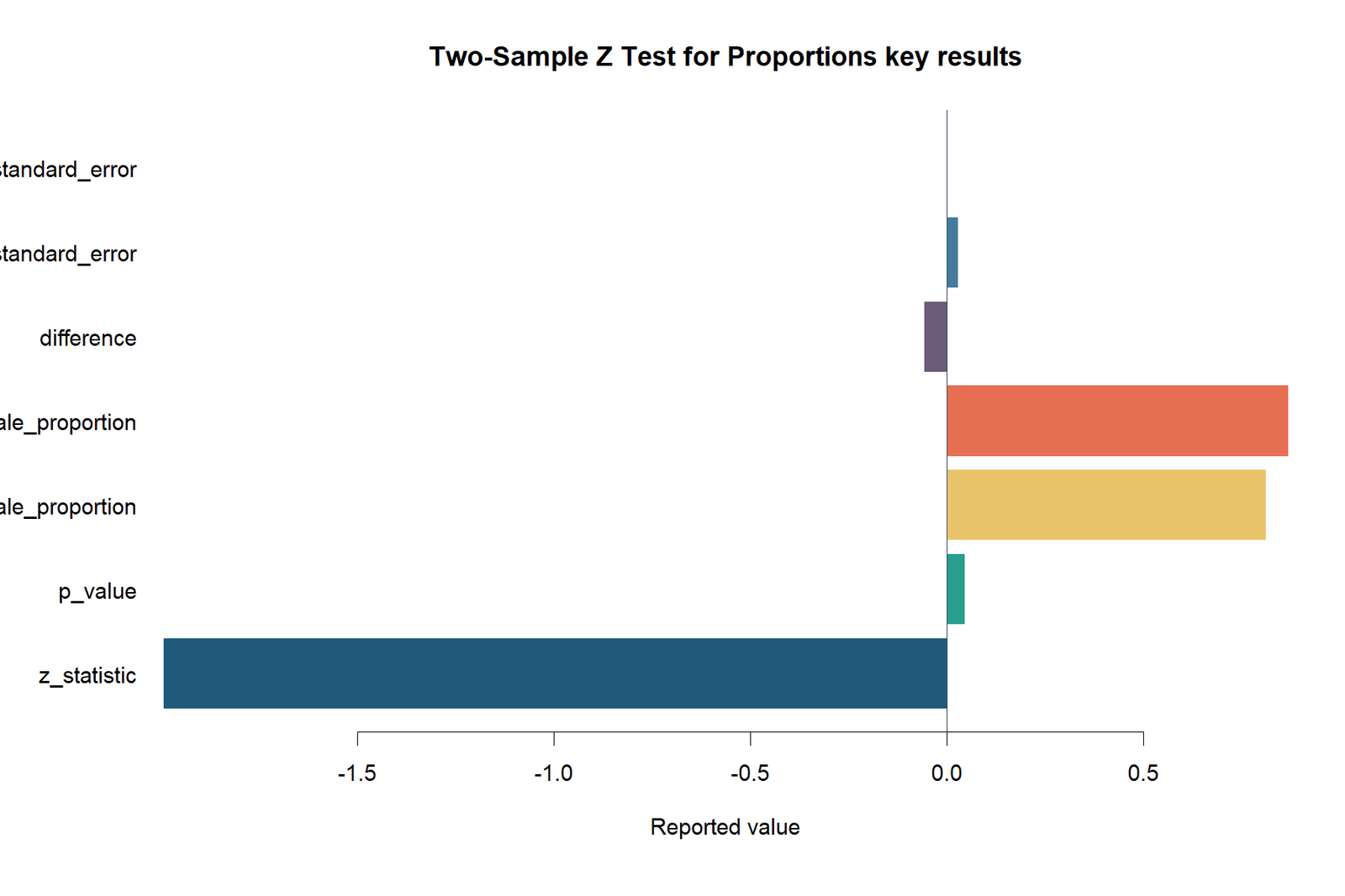
Check: values agree with the workbook and Python output.

Second figure

Z Test Result Summary

The final summary combines the difference, z, p-value and decision, making clear that the result is significant at .05 but close to the boundary.

Check: direction remains male minus female throughout.

Z Test for Proportions in Python, R, SPSS, SAS and Excel

Python

Create arrays x = [216, 333] and n = [266, 383].
Use a two-sided pooled proportions z test.
Verify z = −1.9927455 and p = 0.0462893.
Calculate unpooled intervals separately.

R

Use the score or asymptotic proportion test with correction disabled.
State whether the function reports a chi-square statistic or its signed z equivalent.
Preserve the male-minus-female direction in custom calculations.
Check group intervals independently.

SPSS

Build sex × G3-pass crosstabs.
Request column-proportion comparisons or an uncorrected 2 × 2 test.
Check category order and reference letters.
Reconcile Pearson χ² = 3.9710 with z².

Excel

Enter the four counts in clearly labelled cells.
Calculate p̂ values, pooled p̂, both SEs, z and p.
Use NORM.S.DIST for tail probabilities.
Keep formulas auditable rather than hard-coding results.

Cross-Software Result Reconciliation

Output	Python	R	SPSS/χ² form	Excel	Agreement
Male proportion	0.812030	0.812030	0.812030	0.812030	Exact
Female proportion	0.869452	0.869452	0.869452	0.869452	Exact
Signed z	−1.992745	−1.992745	±√3.971035	−1.992745	Exact after sign convention
Two-sided p	0.046289	0.046289	0.046289	0.046289	Exact
Unpooled SE	0.029499	0.029499	Not always printed	0.029499	Exact where reported

Software Settings That Change the Output

Continuity correction, one-sided versus two-sided alternatives, category order, reference group, exact methods and confidence-interval method can all change the printed result. Reproducible reporting therefore includes the function or dialog choice, correction setting and subtraction direction.

Expandable Z Test for Proportions Code

Python code for the pooled two-proportion z test

from math import sqrt
from statistics import NormalDist

x_m, n_m = 216, 266
x_f, n_f = 333, 383
p_m, p_f = x_m / n_m, x_f / n_f
p_pool = (x_m + x_f) / (n_m + n_f)
se0 = sqrt(p_pool * (1 - p_pool) * (1/n_m + 1/n_f))
z = (p_m - p_f) / se0
p_two = 2 * NormalDist().cdf(-abs(z))
print(p_m, p_f, z, p_two)

R code with the signed z calculation

x1 <- 216; n1 <- 266
x2 <- 333; n2 <- 383
p1 <- x1/n1; p2 <- x2/n2
p_pool <- (x1+x2)/(n1+n2)
se0 <- sqrt(p_pool*(1-p_pool)*(1/n1+1/n2))
z <- (p1-p2)/se0
p_two <- 2*pnorm(-abs(z))
c(p1=p1, p2=p2, z=z, p=p_two)

SPSS syntax outline

* G3PASS is 1 for G3 >= 10 and 0 otherwise.
CROSSTABS
  /TABLES=sex BY G3PASS
  /STATISTICS=CHISQ
  /CELLS=COUNT ROW EXPECTED RESID.

* For a 2x2 table without continuity correction,
* signed z = sign(p_M-p_F) * SQRT(Pearson chi-square).

Excel formulas

Male proportion:      =B2/C2
Female proportion:    =B3/C3
Difference:           =D2-D3
Pooled proportion:    =SUM(B2:B3)/SUM(C2:C3)
Pooled SE:            =SQRT(D5*(1-D5)*(1/C2+1/C3))
Z statistic:          =D4/D6
Two-sided p-value:    =2*(1-NORM.S.DIST(ABS(D7),TRUE))
Unpooled SE:          =SQRT(D2*(1-D2)/C2+D3*(1-D3)/C3)

SAS code outline

proc freq data=students;
  tables sex*g3pass / chisq riskdiff relrisk;
  weight count;
run;

/* Verify whether continuity correction is printed and
   use the uncorrected Pearson 1-df statistic for z^2. */

Code safeguard: do not infer the sign of z from a chi-square table without checking the observed subtraction order. Chi-square is nonnegative and loses direction.

How to Interpret and Report the Z Test for Proportions

Interpretation Sequence

Report First

The two group counts and denominators.
The two observed proportions.
The subtraction direction.
The absolute difference in percentage points.
The z statistic and exact p-value.

Then Qualify

The evidence is borderline at .05.
The standardized effect is small.
The interval is sensitive to method.
The test is unadjusted for other variables.
No causal claim follows from the test alone.

Worked APA-Style Report

A two-sample Z Test for Proportions indicated that the pass proportion was lower for male students (216/266, 81.20%) than for female students (333/383, 86.95%), a difference of −5.74 percentage points, z = −1.99, p = .046, two-sided. The unpooled Wald 95% confidence interval for the male-minus-female difference ranged from −11.52 to 0.04 percentage points. The corresponding standardized 2 × 2 association was small, φ = .078.

Reporting Templates

Replace every highlighted field with the study-specific value and preserve the chosen group order.

Statistically significant result

p < α

Counts

The success proportions were x1/n1 (%) and x2/n2 (%).

Test

A two-sample Z Test for Proportions found a difference, z = value, p = value.

Effect

The absolute difference was percentage points, with a 95% CI of lower to upper.

Non-significant result

p ≥ α

Decision

The analysis did not provide sufficient evidence of unequal proportions, z = value, p = value.

Precision

The interval ranged from lower to upper, showing which effects remain plausible.

Prespecified one-sided result

Directional

Hypothesis

The directional alternative p1 < p2 or p1 > p2 was specified before analysis.

Probability

The one-sided test yielded z = value, p = value.

Never choose a one-sided alternative after observing the direction.

What Not to Say

Avoid	Why it is wrong	Better wording
“Males are 5.74% less likely.”	A 5.74-point difference is not the same as a 5.74% relative reduction.	“The male pass rate was 5.74 percentage points lower.”
“The null is false.”	A p-value does not prove a hypothesis false.	“The data provided evidence against equal proportions.”
“Gender caused the difference.”	The test is unadjusted and noncausal.	“Pass proportion was associated with gender in this sample.”
“p = .046 means a 4.6% chance H0 is true.”	The p-value conditions on H0.	“Under equal proportions, a result this extreme has probability .046.”

Common Z Test for Proportions Mistakes and Corrections

Calculation Mistakes

Pooling for the confidence interval.
Failing to pool for the equality test.
Using percentages without denominators.
Reversing group order mid-calculation.
Doubling the wrong tail probability.
Applying an independent test to paired data.

Interpretation Mistakes

Calling a borderline result “highly significant.”
Equating statistical significance with a large effect.
Ignoring interval-method sensitivity.
Claiming causality from an observational comparison.
Hiding the dichotomisation threshold.
Reporting only p without counts and proportions.

Mistake	Consequence in this example	Correction
Treat 50 failures in each group as equal risk	Ignores n = 266 versus n = 383.	Compare 18.80% with 13.05%.
Use unpooled SE for the null test	Produces a smaller \|z\| and changes the p-value.	Use pooled SE = 0.028815.
Use pooled SE for the interval	Understates estimation uncertainty.	Use unpooled SE = 0.029499.
Round proportions before calculating	Can move a borderline p-value.	Retain full precision until reporting.
Interpret interval overlap visually	Does not equal a direct test.	Calculate the difference and its SE.
Ignore continuity-correction defaults	Software results may appear inconsistent.	Document correction settings.

Most serious error: using this test for before-and-after outcomes from the same students. Paired binary data require the discordant-pair logic of McNemar’s test rather than the independent-group pooled standard error.

Z Test for Proportions Practice Questions

Question 1

Recalculate the male pass proportion.

Answer: 216/266 = 0.812030, or 81.20%.

Question 2

Recalculate the female pass proportion.

Answer: 333/383 = 0.869452, or 86.95%.

Question 3

What is the male-minus-female difference?

Answer: 0.812030 − 0.869452 = −0.057422, or −5.74 percentage points.

Question 4

Why is the pooled proportion 549/649?

Answer: Under H0 the groups share one population proportion, so successes and totals are combined for the null SE.

Question 5

What does z = −1.9927 mean?

Answer: The observed difference is 1.9927 pooled-null standard errors below zero.

Question 6

What is the two-sided decision at α = .05?

Answer: Reject equal proportions because p = .046289 < .05.

Question 7

What is the decision at α = .01?

Answer: Do not reject because .046289 > .01.

Question 8

Why can the unpooled interval include zero while p < .05?

Answer: The test and interval use different standard errors and the result is borderline.

Question 9

Which group contributes the wider proportion interval?

Answer: Males, because n = 266 is smaller than n = 383.

Question 10

What is the equivalent Pearson chi-square statistic?

Answer: z² = 3.971035 with 1 degree of freedom.

Question 11

Would McNemar’s test be appropriate?

Answer: No, not for independent male and female groups; it is for paired binary outcomes.

Question 12

At G3 ≥ 12, what is the observed difference?

Answer: 45.49% male versus 59.27% female, a difference of −13.78 percentage points.

Z Test for Proportions Reports and Worked Files

Use the reports to verify software output and the workbook to audit every formula from raw data through reporting.

Python analysis reportCounts, proportions, test statistic, charts and interpretation.R analysis reportIndependent R verification and visual output.SPSS output PDFCrosstabs, chi-square equivalence and supporting output.Worked Excel analysisRaw data, formulas, diagnostics and reporting sheet.

Reproducibility check: the Excel workbook reports male proportion 0.8120300752, female proportion 0.8694516971, z = −1.9927454994 and p = 0.0462893224, matching the independently verified references.

Z Test for Proportions Frequently Asked Questions

What is a Z Test for Proportions?

It is a standard-normal test for one population proportion or the difference between two independent population proportions.

Why is the two-sample test pooled?

Under the equality null, both groups are assumed to share one population proportion, so the best null estimate combines successes and totals.

Why is the confidence interval unpooled?

The interval estimates the actual difference without imposing equal proportions, so each group contributes its own estimated variance.

What are the conditions for a two-proportion Z test?

Binary outcomes, independent groups and observations, transparent sampling, and sufficiently large null-expected success and failure counts.

What does a negative z value mean?

It means the first group proportion is below the second under the stated subtraction order.

Is p = .046 strong evidence?

It crosses .05 but is close to the threshold. It should be described as modest or borderline evidence, not overwhelming evidence.

Why does the Wald interval include zero?

The interval uses the slightly larger unpooled standard error, while the test uses the pooled null standard error.

Is the Z Test for Proportions the same as chi-square?

For an uncorrected 2 × 2 table, the two-proportion z statistic squared equals the one-degree-of-freedom Pearson chi-square statistic.

Can I use this test for paired data?

No. Use McNemar’s test for the same people measured twice or matched pairs.

Should I report relative risk too?

It is useful when a ratio interpretation matters, but it complements rather than replaces the absolute difference and z test.

Does statistical significance prove causation?

No. Causal interpretation depends on design, assignment, sampling and control of confounding.

What is the main worked conclusion?

Male pass proportion was 81.20% and female pass proportion was 86.95%; z = −1.99, p = .046, two-sided.

Z Test for Proportions Conclusion

The Z Test for Proportions transformed a 5.74-percentage-point male–female pass-rate gap into a pooled-null z statistic of −1.992745. The two-sided p-value of 0.046289 crosses the conventional .05 threshold, so the equality null is rejected at that level. Female students had the higher observed pass proportion: 86.95% compared with 81.20% for males.

The most important analytical lesson is the separation between testing and estimation. The equality test pools the proportions and uses SE = 0.028815, while the difference interval does not pool and uses SE = 0.029499. Because the evidence is near the threshold, that distinction visibly affects the conclusion drawn from different interval methods. Reporting the exact counts, exact p-value, absolute difference, confidence interval, effect size and software settings gives a more honest account than a significance label alone.

Final reporting sentence: “Male students had a lower G3 pass proportion than female students (81.20% vs. 86.95%), a difference of −5.74 percentage points, z = −1.99, p = .046, two-sided; the standardized association was small, φ = .078.”

AdvertisementGoogle AdSense bottom placement reserved here

↑Back to top

Z Test for Proportions: Formula, Example, Interpretation, Python, R, SPSS, SAS and Excel Guide

Z Test for Proportions Model Overview

The Exact Research Question

Why Two Standard Errors Appear

Quick Answer: Z Test for Proportions Result

Statistical Decision

Data Meaning

Table of Contents

What Is a Z Test for Proportions?

One-Sample and Two-Sample Forms

What Is Being Standardized?

What the Test Does Not Prove

Research Question, Hypotheses and Data Design

Research Question

Why the Direction Must Be Declared Before Testing

When to Use the Z Test for Proportions

Use It When

Choose Another Method When

Decision Flow

Z Test for Proportions Variants and Their Meanings

Pooled Does Not Mean the Groups Are Permanently Combined

Continuity Correction

Correction and Method Sensitivity

Variables, Coding and Data Dictionary

Sample Composition

Why the Equal Failure Counts Do Not Mean Equal Failure Rates

Binary coding rule

Subtraction order

Z Test for Proportions Formula and Manual Calculation

Notation Used in the Two-Proportion Formula

Step 1: Compute the Group Proportions

Step 2: Compute the Observed Difference

Step 3: Pool the Proportions Under H0

Null Allocation by Group

Step 4: Compute the Pooled Null Standard Error

Step 5: Compute the Z Statistic

Step 6: Convert Z to a Probability

Step 7: Build a Difference Confidence Interval

Observed Tables, Expected Counts and Raw-Data Profiles

Observed 2 × 2 Table

Expected Counts Under Equal Proportions

Group-Specific Proportion Intervals

Raw G3 Score Distribution by Gender

Original G3 Descriptive Statistics

Threshold Sensitivity

Threshold Pattern Summary

Complete Z Test for Proportions Results

Primary Result Table

Inference on Multiple Scales

Confidence-Interval Comparison

Unpooled Variance Contributions

Why the P-Value and Wald Interval Straddle the .05 Boundary Differently

Z Test for Proportions Assumptions and Diagnostic Checks

Success-Failure Condition Audit

Observed-to-Expected Deviations

Independence Is a Design Condition

Effect of Dichotomising G3

Z Test for Proportions Versus Related Tests

Equivalence with the Pearson 2 × 2 Test

Why Relative Risk and Odds Ratio Do Not Replace the Z Test

Z Test for Proportions Calculator: Step-by-Step Workflow

Calculator Workflow

Result Verification Checklist

Python Z Test for Proportions Chart Interpretations

1Observed 2 × 2 Table

2Male and Female Pass Proportions

3Group-Specific 95% Intervals

4Pooled and Unpooled Standard Errors

5Z Test Result Summary

R Z Test for Proportions Charts in Paired Rows

Observed 2 × 2 Table

Male and Female Pass Proportions

Group-Specific 95% Intervals

Pooled and Unpooled Standard Errors

Standard-Normal Reference

Z Test Result Summary

Z Test for Proportions in Python, R, SPSS, SAS and Excel

Python

R

SPSS

Step 3: Pool the Proportions Under H₀