
Planned Comparisons, ANOVA Contrasts, Coefficients and p-value Decisions
Contrast Analysis: Formula, Interpretation, SPSS, Python, R and Excel Guide
Contrast Analysis is used when the researcher has planned comparisons among group means before or during ANOVA interpretation. Instead of comparing every possible pair blindly, contrast analysis tests exact questions using contrast coefficients. In this worked Salar Cafe example, G3 final grade is compared across four studytime groups using planned contrasts for linear trend, lower versus higher studytime, first group versus later groups and last group versus earlier groups.
Quick Answer: Contrast Analysis Result
The Contrast Analysis result shows that three planned comparisons are statistically significant at α = .05. The first group vs all later groups contrast is significant, the lower groups vs higher groups contrast is significant, and the linear trend across ordered groups contrast is significant. The last group vs all earlier groups contrast is not significant because its p-value is slightly above .05.
The mean profile shows a clear increase from studytime group 1 to studytime group 3, with studytime group 4 remaining high but not clearly higher than all earlier groups. That is why the linear trend and lower-versus-higher comparisons are significant, while the last-group endpoint contrast is not significant.
Final interpretation: G3 increases meaningfully across ordered studytime groups. The strongest planned result is that studytime group 1 is lower than the later studytime groups. The endpoint test comparing the last group against all earlier groups is not significant, so the conclusion should focus on the overall ordered increase and lower-versus-higher studytime difference rather than claiming group 4 is uniquely higher than all previous groups.
Important reporting point: Contrast Analysis is strongest when the comparisons are planned before looking at the data. It is different from post hoc testing because each coefficient pattern represents a specific research question.
Table of Contents
- What Is Contrast Analysis?
- Contrast Analysis Formula
- Planned Contrast Coefficients Used
- Contrast Analysis Hypotheses
- Dataset and Variables Used
- Assumptions Before Contrast Analysis
- SPSS Output Interpretation
- Python Chart-by-Chart Interpretation
- R Chart-by-Chart Validation
- SPSS, R, Python and Excel Workflows
- Code Blocks for Contrast Analysis
- APA Reporting Wording
- Common Mistakes
- When to Use Contrast Analysis
- Downloads and Resources
- Related Guides
- FAQs
What Is Contrast Analysis?
Contrast Analysis is a planned comparison method used to test specific differences or patterns among group means. In ANOVA, the omnibus F test tells whether at least one group mean differs, but it does not always answer the exact research question. A planned contrast lets the researcher test a focused hypothesis, such as whether higher studytime groups outperform lower studytime groups or whether a linear trend appears across ordered categories.
A contrast is built from coefficients assigned to each group. The coefficients usually sum to zero. Positive coefficients represent one side of the comparison, negative coefficients represent the other side, and zero coefficients can exclude groups when needed. The contrast estimate is the weighted sum of the group means.
In this example, the factor is studytime with four ordered groups. The outcome is G3 final grade. The planned contrasts test four research questions: whether there is a linear trend across studytime, whether lower studytime groups differ from higher studytime groups, whether the first group differs from all later groups, and whether the last group differs from all earlier groups.
Simple definition: Contrast Analysis tests planned, coefficient-based questions about group means. It is more focused than a general ANOVA table and more targeted than running every possible post hoc comparison.
This guide connects naturally with One Way ANOVA, Factorial ANOVA, ANOVA in SPSS, ANOVA in R, ANOVA in Python, P Value, Confidence Interval, Null and Alternative Hypothesis and Effect Size.
Contrast Analysis Formula
The contrast estimate is the weighted sum of group means:
Here, L is the contrast estimate, cj is the contrast coefficient for group j, and X̄j is the mean for group j. For a valid standard contrast, the coefficients usually satisfy this condition:
The standard error of the contrast is calculated from the mean square error and the group sample sizes:
The t statistic for the contrast is:
The contrast is statistically significant when the p-value is below the chosen alpha level, commonly .05. In this example, three contrasts have p-values below .05 and one contrast has p = .06705, so it is not significant at the conventional .05 level.
Planned Contrast Coefficients Used
The planned contrast coefficients define the exact comparison being tested. Each row below is a separate planned question. The signs and sizes of the coefficients matter because they control which groups are compared and how strongly each group contributes to the contrast estimate.
| Contrast | Group 1 | Group 2 | Group 3 | Group 4 | Research Question |
|---|---|---|---|---|---|
| Linear trend across ordered groups | -3 | -1 | 1 | 3 | Does G3 increase linearly as studytime rises? |
| Lower groups vs higher groups | -1 | -1 | 1 | 1 | Do higher studytime groups outperform lower studytime groups? |
| First group vs all later groups | 3 | -1 | -1 | -1 | Is the first studytime group different from the later groups? |
| Last group vs all earlier groups | -1 | -1 | -1 | 3 | Is the last studytime group different from all earlier groups? |
Contrast Estimate Summary
| Contrast | Estimate | Approx. 95% CI | p-value | Decision | Interpretation |
|---|---|---|---|---|---|
| First group vs all later groups | -5.843 | -7.63 to -4.06 | 2.516e-10 | Significant | Group 1 is clearly lower than later groups combined. |
| Lower groups vs higher groups | 3.348 | 2.02 to 4.68 | 9.565e-07 | Significant | Higher studytime groups exceed lower studytime groups. |
| Linear trend across ordered groups | 7.773 | 4.34 to 11.21 | 1.034e-05 | Significant | There is a positive ordered studytime trend. |
| Last group vs all earlier groups | 3.008 | -0.21 to 6.23 | .06705 | Not significant | Group 4 is not significantly higher than all earlier groups combined. |
Main result: The significant planned contrasts support an ordered improvement in G3 across studytime, especially the difference between the lowest studytime group and the later groups. The last group endpoint comparison does not reach p < .05.
Contrast Analysis Hypotheses
Each contrast has its own hypothesis. The null hypothesis says that the weighted group mean comparison equals zero. The alternative hypothesis says that the weighted comparison is different from zero.
| Contrast | Null Hypothesis | Alternative Hypothesis | Decision in This Output |
|---|---|---|---|
| Linear trend | The ordered contrast equals zero. | There is a nonzero ordered trend. | Reject H0. |
| Lower vs higher | Lower and higher studytime sets do not differ. | Lower and higher studytime sets differ. | Reject H0. |
| First vs later | Group 1 does not differ from later groups. | Group 1 differs from later groups. | Reject H0. |
| Last vs earlier | Group 4 does not differ from earlier groups. | Group 4 differs from earlier groups. | Fail to reject H0. |
Decision for this example: Three planned contrasts are statistically significant. The last group versus all earlier groups contrast is not significant, so the report should not claim that studytime group 4 is uniquely different from all earlier groups.
Dataset and Variables Used
The worked example uses student performance data. The dependent variable is G3 final grade. The grouping variable is studytime, which has four ordered levels. The contrast analysis uses the same group means that appear in the ANOVA and post hoc workflow.
| Variable | Role | Levels / Type | Why It Matters |
|---|---|---|---|
| G3 | Dependent variable | Numeric final grade | The outcome compared across studytime groups. |
| studytime | Grouping factor | 1, 2, 3, 4 | The ordered groups used for planned contrasts. |
Group Mean Pattern
| Studytime Group | Mean G3 | Interpretation |
|---|---|---|
| 1 | 10.8443 | Lowest mean G3; drives the first-vs-later contrast. |
| 2 | 12.0918 | Higher than group 1 but lower than group 3. |
| 3 | 13.2268 | Highest mean G3 in the profile. |
| 4 | 13.0571 | High mean but close to group 3, so endpoint contrast is not significant. |
The mean profile is the key to interpretation. Studytime group 1 is clearly lower. Groups 3 and 4 are both high, but group 4 is not clearly above group 3. That pattern explains why the linear and lower-versus-higher contrasts are significant, while the last-group endpoint contrast is not significant.
For supporting concepts, review Descriptive Statistics, Mean Median and Mode, Standard Deviation, Standard Error, Confidence Interval, Five Number Summary, Box Plot Interpretation and Histogram Interpretation.
Assumptions Before Contrast Analysis
Contrast Analysis uses the ANOVA error term, so the usual ANOVA assumptions still matter. The outcome should be numeric, the groups should be independent, and the residual variation should be suitable for the planned comparison model.
| Assumption | Meaning | How This Example Handles It |
|---|---|---|
| Continuous outcome | The dependent variable should be numeric. | G3 is a numeric final-grade variable. |
| Categorical grouping factor | The independent variable should define groups. | Studytime defines four groups. |
| Independent observations | Each observation should contribute one independent score. | Each student contributes one G3 value. |
| Planned comparisons | Contrasts should answer specific research questions. | Four planned patterns were tested. |
| Coefficient sum | Standard contrasts usually sum to zero. | All four contrast coefficient sets sum to zero. |
| ANOVA assumptions | Variance and residual assumptions should be checked. | Use ANOVA assumption diagnostics before final reporting. |
For assumption support, use ANOVA Assumptions, Levene Test, Bartlett’s Test, Brown-Forsythe Test, Q-Q Plot Normality Check, P-P Plot Normality Check, Shapiro-Wilk Test and Outlier Detection.
SPSS Output Interpretation for Contrast Analysis
The SPSS output for Contrast Analysis should be read in a sequence: first the descriptive group means, then the ANOVA context, then the planned contrast table. The planned contrast table is more important than a general post hoc table because the contrasts represent specific coefficient-based research questions.
SPSS Reading Order
| SPSS Output Area | What to Read | Why It Matters |
|---|---|---|
| Descriptives | Mean G3 by studytime group | Shows the group pattern behind the contrasts. |
| ANOVA table | Overall group difference | Provides the model error term used by contrasts. |
| Contrast coefficients | Coefficient values for each group | Defines each planned comparison exactly. |
| Contrast tests | Estimate, standard error, t value and p-value | Main decision table for planned comparisons. |
| Confidence intervals | Whether the interval crosses zero | Confirms significance and direction. |
SPSS Planned Contrast Interpretation
| Contrast | Meaning | Result | SPSS Reporting Decision |
|---|---|---|---|
| Linear trend | Tests ordered increase across studytime groups. | Significant | Report a positive planned trend in G3. |
| Lower vs higher | Compares studytime groups 1–2 against 3–4. | Significant | Report higher G3 for higher studytime groups. |
| First vs later | Compares group 1 against groups 2–4 combined. | Significant | Report group 1 as lower than later groups. |
| Last vs earlier | Compares group 4 against groups 1–3 combined. | Not significant | Do not claim group 4 is uniquely different from all earlier groups. |
SPSS interpretation summary: The planned contrast output supports an ordered studytime pattern and a strong first-group disadvantage. The last-group endpoint contrast is not significant, so the final interpretation should be about the overall ordered increase rather than an isolated advantage for group 4.
Python Chart-by-Chart Interpretation
The Python chart sequence explains Contrast Analysis through group distributions, group mean profile, planned contrast coefficients, contrast estimates with confidence intervals and p-value decisions.
Python Chart 1: Group Distribution Boxplots
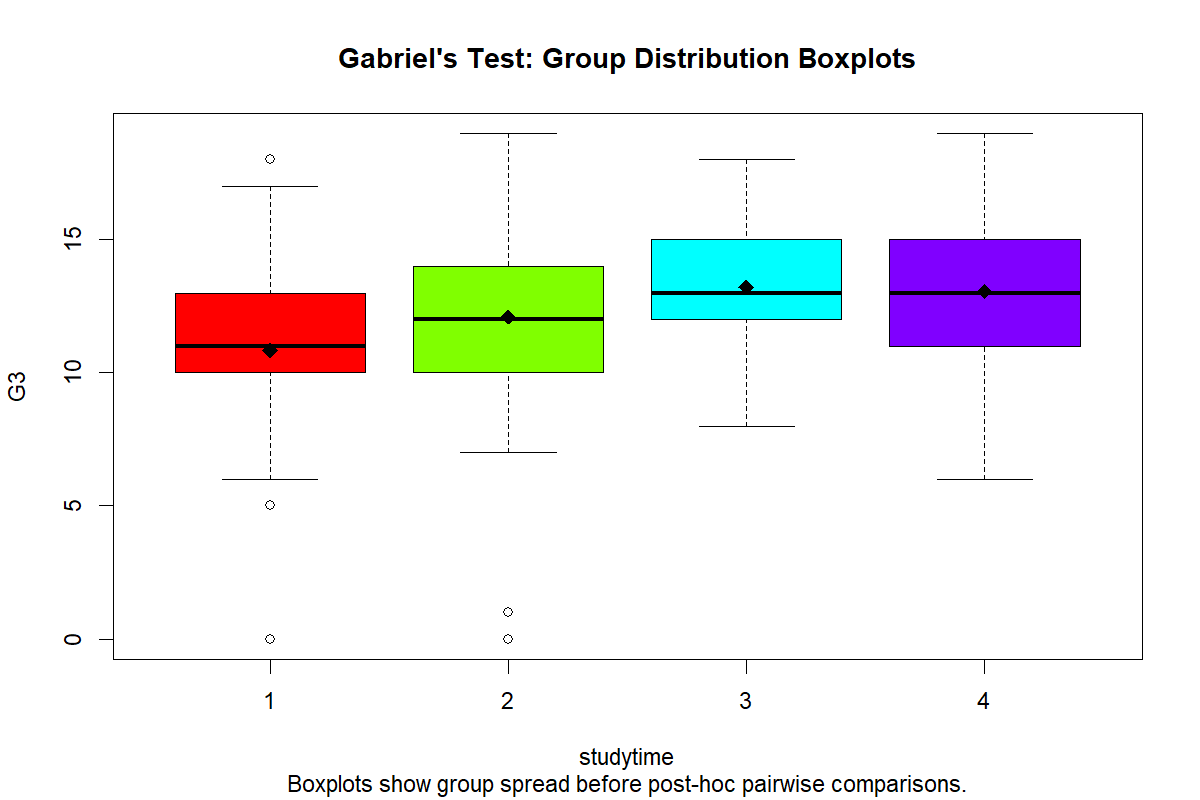
The boxplots show that the lower studytime groups have lower central G3 values, while studytime groups 3 and 4 appear higher. This distribution pattern supports the planned comparisons that compare lower studytime against higher studytime.
The boxplot is important because contrast analysis should not be interpreted only from a p-value table. The visual distribution shows whether the planned question matches the real group pattern.
Python Chart 2: Group Mean Profile
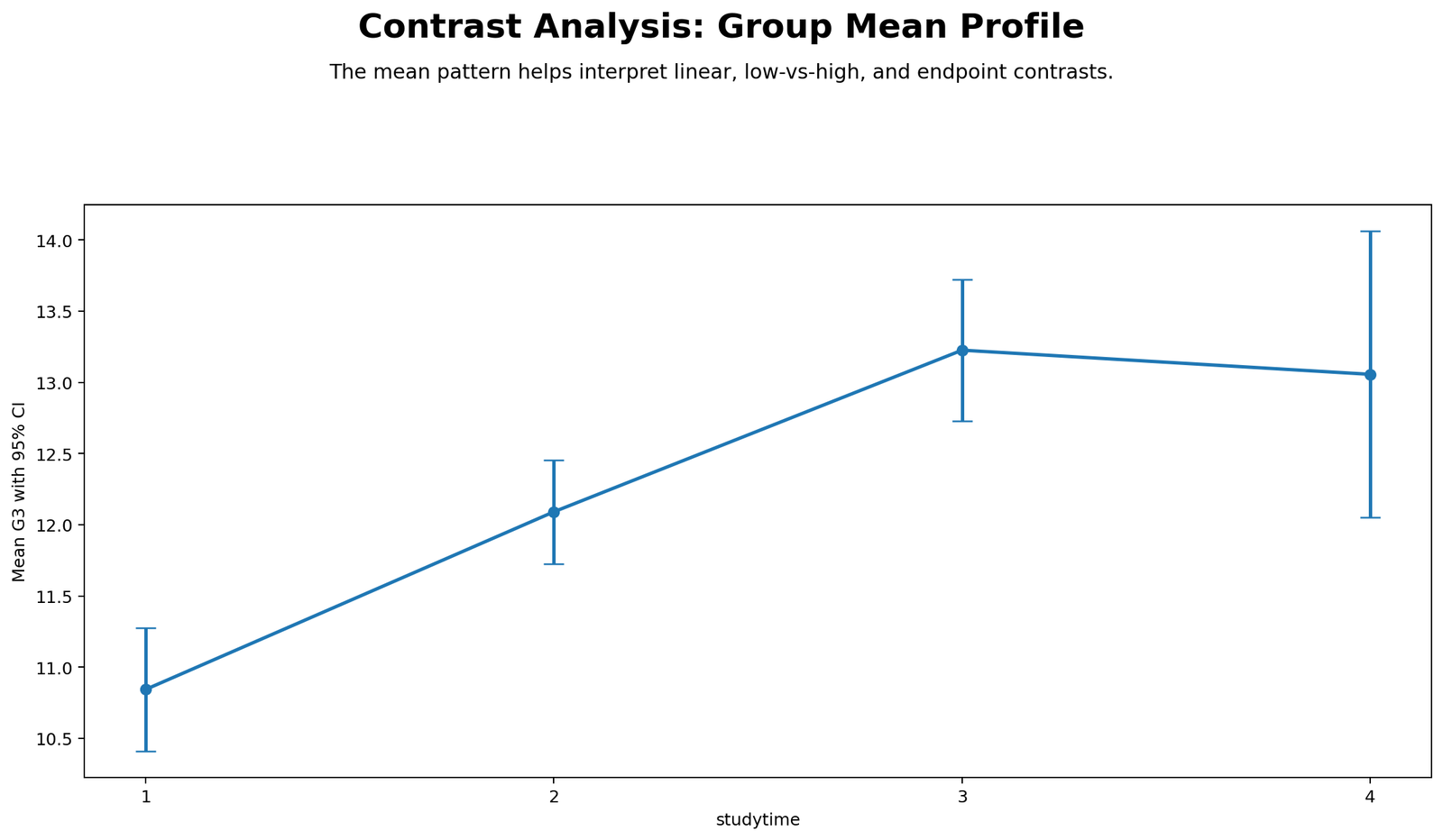
The mean profile rises from group 1 to group 3 and then remains high at group 4. This pattern explains why the linear trend contrast is significant. It also explains why lower-versus-higher studytime is significant.
The chart also prevents overinterpretation. Group 4 is not visibly much higher than group 3, so the last-group-versus-earlier-groups contrast is weaker and does not reach the .05 significance level.
Python Chart 3: Planned Contrast Coefficients
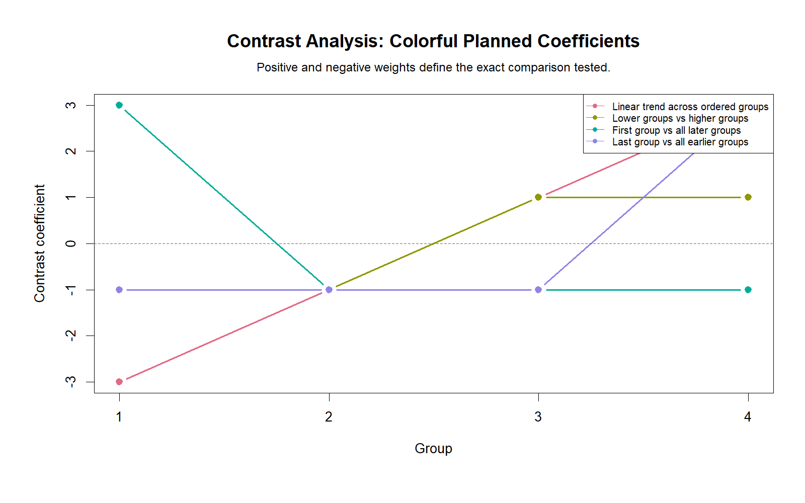
The coefficient plot shows the structure of each planned comparison. The linear trend uses -3, -1, 1 and 3 to test an ordered increase. The lower-versus-higher contrast uses -1, -1, 1 and 1. The first-versus-later contrast uses 3, -1, -1 and -1. The last-versus-earlier contrast uses -1, -1, -1 and 3.
This chart is central to contrast analysis because the coefficients are the test. Different coefficients answer different research questions even when they use the same group means.
Python Chart 4: Contrast Estimates with Confidence Intervals
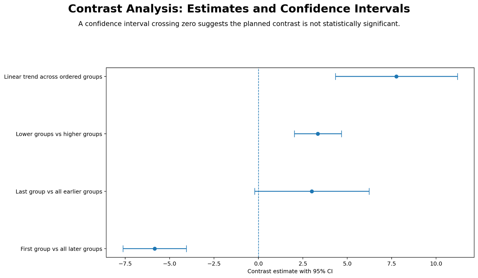
The confidence-interval chart shows which planned comparisons are clearly different from zero. The first-versus-later contrast is below zero and its interval does not cross zero. The lower-versus-higher and linear trend contrasts are above zero and their intervals do not cross zero.
The last-versus-earlier contrast has an interval that crosses zero. This matches the non-significant p-value and supports the decision not to interpret group 4 as uniquely different from all earlier groups.
Python Chart 5: Contrast p-value Decision Plot
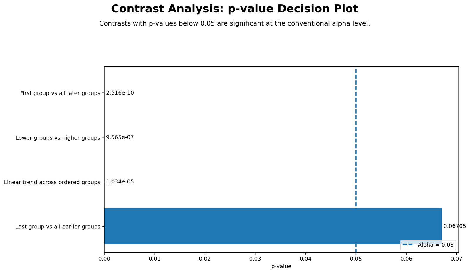
The p-value decision chart shows that three contrasts fall below the α = .05 threshold: first group vs all later groups, lower groups vs higher groups and linear trend across ordered groups.
The last group vs all earlier groups contrast has p = .06705, which is above .05. The correct reporting decision is to call this contrast not significant at the conventional alpha level.
R Chart-by-Chart Validation
The R charts validate the same Contrast Analysis workflow using a second software environment. The R output confirms the same distribution pattern, group mean profile, planned coefficients, confidence-interval interpretation and p-value decision pattern.
R Chart 1: Group Distribution Boxplots
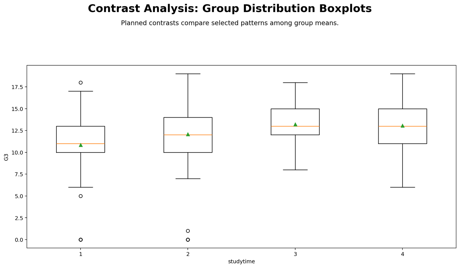
The R boxplot confirms the same descriptive pattern as Python. Studytime group 1 has a lower central value, while groups 3 and 4 are higher.
This validation supports the planned contrast interpretation because the visual pattern is consistent across software outputs.
R Chart 2: Group Mean Profile
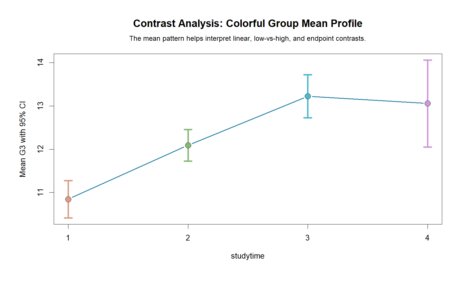
The R group mean profile confirms that mean G3 increases from group 1 to group 3, with group 4 remaining high. The profile supports the significant linear trend and lower-versus-higher planned contrasts.
The same chart also explains why the endpoint comparison for group 4 is not significant. Group 4 is high, but it is not clearly higher than every earlier group.
R Chart 3: Planned Contrast Coefficients
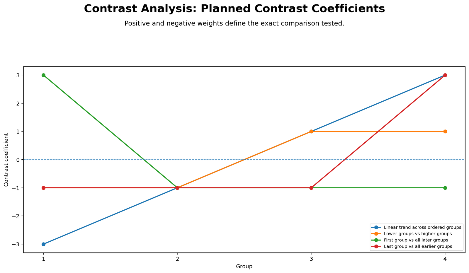
The R coefficient chart confirms the same contrast designs used in the Python workflow. Each colored line represents a different planned comparison.
This is useful for readers because coefficients can be abstract in a table. The chart shows exactly which groups receive negative weights and which groups receive positive weights.
R Chart 4: Contrast Estimates with Confidence Intervals
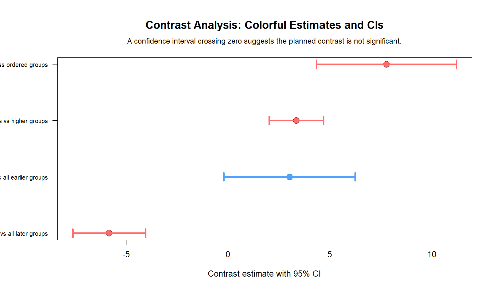
The R estimate chart confirms that the first-versus-later, lower-versus-higher and linear trend contrasts have confidence intervals that do not cross zero.
The last-versus-earlier contrast crosses zero, so it is not statistically significant. This confirms the same decision shown in the Python chart.
R Chart 5: Contrast p-value Decision Plot
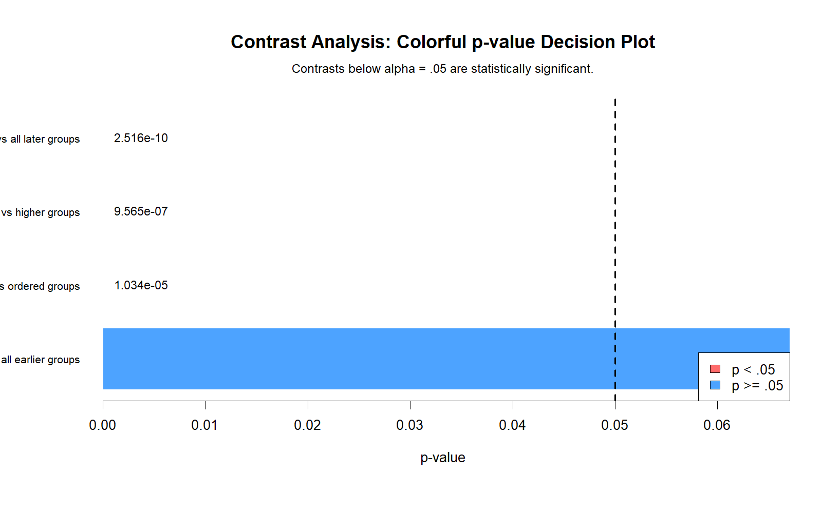
The R p-value plot confirms that three planned contrasts are significant and one is not significant. The p-values match the same decision pattern as Python.
This agreement across Python, R and SPSS strengthens the final article conclusion: the planned contrast analysis supports an ordered studytime effect but does not support a unique last-group endpoint effect.
SPSS, R, Python and Excel Workflows for Contrast Analysis
The same Contrast Analysis workflow can be reproduced in SPSS, R, Python and Excel. SPSS can run planned contrasts through one-way ANOVA contrast settings. R can use custom contrasts with lm(), aov() or contrast matrices. Python can calculate contrast estimates from group means and the ANOVA error term. Excel can calculate the contrast estimate, standard error, t statistic, p-value and confidence interval manually.
SPSS Workflow
| Step | SPSS Menu or Syntax | Purpose |
|---|---|---|
| Open dataset | File > Open > Data | Load G3 and studytime. |
| Run One-Way ANOVA | Analyze > Compare Means > One-Way ANOVA | Set up the ANOVA model. |
| Dependent variable | G3 | Outcome variable. |
| Factor | studytime | Grouping variable. |
| Contrasts | Enter planned coefficients | Define each planned comparison. |
| Output | Contrast coefficients and contrast tests | Read estimates, t values and p-values. |
R Workflow
| Step | R Action | Purpose |
|---|---|---|
| Read data | read.csv("dataset.csv") | Load the dataset. |
| Convert group | factor(studytime) | Define studytime as a factor. |
| Calculate group means | group_by(studytime) | Prepare contrast estimates. |
| Fit ANOVA model | aov(G3 ~ studytime) | Get the model error term. |
| Define contrast matrix | Coefficient matrix | Define planned comparisons. |
| Test contrasts | Estimate, SE, t, p and CI | Report each planned comparison. |
Python Workflow
| Step | Python Action | Purpose |
|---|---|---|
| Read data | pandas.read_csv() | Load G3 and studytime. |
| Run ANOVA | statsmodels or scipy | Estimate MSE and degrees of freedom. |
| Define coefficients | Dictionary or matrix of contrast weights | Create planned contrasts. |
| Calculate estimate | sum(c * mean) | Get the contrast estimate. |
| Calculate SE | sqrt(MSE * sum(c^2/n)) | Get standard error. |
| Decision | t statistic, p-value and confidence interval | Interpret significance and direction. |
Excel Workflow
| Excel Task | Formula or Tool | Purpose |
|---|---|---|
| Prepare data | Columns for G3 and studytime | Organize the dataset. |
| Group means | PivotTable average of G3 by studytime | Calculate group means. |
| Group counts | PivotTable count of G3 by studytime | Calculate n for each group. |
| Enter coefficients | Manual coefficient row | Define the planned contrast. |
| Contrast estimate | =SUMPRODUCT(coefficients,means) | Calculate L. |
| Standard error | =SQRT(MSE*SUM(coefficients^2/n)) | Calculate SE(L). |
| t statistic | =estimate/SE | Test the contrast. |
| p-value | =T.DIST.2T(ABS(t),df) | Make the significance decision. |
Code Blocks for Contrast Analysis
SPSS Syntax for Contrast Analysis
* Contrast Analysis in SPSS.
* Dependent variable: G3.
* Grouping factor: studytime.

TITLE "Contrast Analysis: G3 by Studytime".

ONEWAY G3 BY studytime
  /STATISTICS DESCRIPTIVES HOMOGENEITY
  /CONTRAST = -3 -1 1 3
  /CONTRAST = -1 -1 1 1
  /CONTRAST = 3 -1 -1 -1
  /CONTRAST = -1 -1 -1 3
  /MISSING ANALYSIS.

EXAMINE VARIABLES=G3 BY studytime
  /PLOT BOXPLOT
  /COMPARE GROUPS
  /STATISTICS DESCRIPTIVES
  /CINTERVAL 95
  /MISSING LISTWISE
  /NOTOTAL.

OUTPUT EXPORT
  /CONTENTS EXPORT=VISIBLE
  /PDF DOCUMENTFILE="Contrast-Analysis-SPSS-Output.pdf".
Python Code for Contrast Analysis
import pandas as pd
import numpy as np
from scipy import stats
from statsmodels.formula.api import ols
from statsmodels.stats.anova import anova_lm

df = pd.read_csv("dataset.csv")

df["G3"] = pd.to_numeric(df["G3"], errors="coerce")
df["studytime"] = df["studytime"].astype("category")

data = df[["G3", "studytime"]].dropna().copy()

# ANOVA model for MSE
model = ols("G3 ~ C(studytime)", data=data).fit()
anova_table = anova_lm(model, typ=2)

mse = anova_table.loc["Residual", "sum_sq"] / anova_table.loc["Residual", "df"]
df_error = anova_table.loc["Residual", "df"]

summary = data.groupby("studytime", observed=True)["G3"].agg(
    n="count",
    mean="mean",
    sd="std"
).reset_index()

print(summary)
print(anova_table)

means = summary.set_index("studytime")["mean"].to_dict()
counts = summary.set_index("studytime")["n"].to_dict()

contrasts = {
    "Linear trend across ordered groups": {"1": -3, "2": -1, "3": 1, "4": 3},
    "Lower groups vs higher groups": {"1": -1, "2": -1, "3": 1, "4": 1},
    "First group vs all later groups": {"1": 3, "2": -1, "3": -1, "4": -1},
    "Last group vs all earlier groups": {"1": -1, "2": -1, "3": -1, "4": 3}
}

rows = []

for name, coeffs in contrasts.items():
    estimate = sum(coeffs[g] * means[g] for g in coeffs)
    se = np.sqrt(mse * sum((coeffs[g] ** 2) / counts[g] for g in coeffs))
    t_value = estimate / se
    p_value = 2 * (1 - stats.t.cdf(abs(t_value), df_error))
    t_crit = stats.t.ppf(0.975, df_error)
    ci_low = estimate - t_crit * se
    ci_high = estimate + t_crit * se

    rows.append({
        "contrast": name,
        "estimate": estimate,
        "standard_error": se,
        "t_value": t_value,
        "df": df_error,
        "p_value": p_value,
        "ci_low": ci_low,
        "ci_high": ci_high,
        "decision": "Significant" if p_value < 0.05 else "Not significant"
    })

contrast_table = pd.DataFrame(rows)
print(contrast_table)
R Code for Contrast Analysis
# Contrast Analysis in R

library(tidyverse)
library(car)

df <- read.csv("dataset.csv")

df$G3 <- as.numeric(df$G3)
df$studytime <- as.factor(df$studytime)

data <- df %>%
  select(G3, studytime) %>%
  drop_na()

# Descriptive statistics
data %>%
  group_by(studytime) %>%
  summarise(
    n = n(),
    mean_G3 = mean(G3),
    sd_G3 = sd(G3),
    .groups = "drop"
  )

# ANOVA model
model <- aov(G3 ~ studytime, data = data)
summary(model)

# Planned contrast matrix
contrast_matrix <- matrix(
  c(
    -3, -1,  1,  3,
    -1, -1,  1,  1,
     3, -1, -1, -1,
    -1, -1, -1,  3
  ),
  nrow = 4,
  byrow = TRUE
)

rownames(contrast_matrix) <- c(
  "Linear trend across ordered groups",
  "Lower groups vs higher groups",
  "First group vs all later groups",
  "Last group vs all earlier groups"
)

colnames(contrast_matrix) <- levels(data$studytime)

# Manual contrast estimates
group_summary <- data %>%
  group_by(studytime) %>%
  summarise(n = n(), mean_G3 = mean(G3), .groups = "drop")

mse <- summary(model)[[1]]["Residuals", "Mean Sq"]
df_error <- summary(model)[[1]]["Residuals", "Df"]

results <- lapply(1:nrow(contrast_matrix), function(i) {
  coeffs <- contrast_matrix[i, ]
  estimate <- sum(coeffs * group_summary$mean_G3)
  se <- sqrt(mse * sum((coeffs^2) / group_summary$n))
  t_value <- estimate / se
  p_value <- 2 * pt(abs(t_value), df = df_error, lower.tail = FALSE)
  t_crit <- qt(.975, df = df_error)
  data.frame(
    contrast = rownames(contrast_matrix)[i],
    estimate = estimate,
    standard_error = se,
    t_value = t_value,
    df = df_error,
    p_value = p_value,
    ci_low = estimate - t_crit * se,
    ci_high = estimate + t_crit * se,
    decision = ifelse(p_value < .05, "Significant", "Not significant")
  )
})

bind_rows(results)
Excel Notes for Contrast Analysis
Excel support workflow:

1. Arrange the data:
   G3 | studytime

2. Create a PivotTable:
   Rows = studytime
   Values = average of G3 and count of G3

3. Enter group means:
   Group 1 mean
   Group 2 mean
   Group 3 mean
   Group 4 mean

4. Enter contrast coefficients:
   Linear trend: -3, -1, 1, 3
   Lower vs higher: -1, -1, 1, 1
   First vs later: 3, -1, -1, -1
   Last vs earlier: -1, -1, -1, 3

5. Check coefficient sum:
   =SUM(coefficient_row)
   This should equal 0.

6. Calculate contrast estimate:
   =SUMPRODUCT(coefficient_row, mean_row)

7. Calculate standard error:
   =SQRT(MSE*SUM(coefficients^2/group_counts))

8. Calculate t statistic:
   =contrast_estimate/standard_error

9. Calculate p-value:
   =T.DIST.2T(ABS(t_statistic), error_df)

10. Decision:
   =IF(p_value<0.05,"Significant","Not significant")
APA Reporting Wording
When reporting Contrast Analysis, state that planned contrasts were used, describe the coefficients or the research question behind each contrast, and report the estimate, confidence interval, test statistic or p-value.
APA-style report: Planned contrast analysis was conducted to compare G3 final grade across ordered studytime groups. A significant linear trend was found across the four ordered studytime levels, p = 1.034e-05, indicating that G3 increased as studytime increased. The lower-versus-higher studytime contrast was also significant, estimate = 3.348, 95% CI [2.02, 4.68], p = 9.565e-07. The first group versus all later groups contrast was significant, estimate = -5.843, 95% CI [-7.63, -4.06], p = 2.516e-10, showing that studytime group 1 had lower G3 than later studytime groups. The last group versus all earlier groups contrast was not significant, estimate = 3.008, 95% CI [-0.21, 6.23], p = .06705.
Short reporting version: Planned contrasts showed a significant positive studytime trend and a significant lower-versus-higher studytime difference. Studytime group 1 was significantly lower than the later groups, but studytime group 4 was not significantly different from all earlier groups combined.
Common Mistakes
| Mistake | Why It Is Wrong | Correct Practice |
|---|---|---|
| Using contrasts without a planned question | Contrasts are meant to test specific hypotheses. | Define the comparison before reporting it. |
| Forgetting that coefficients should sum to zero | Invalid coefficients can distort the interpretation. | Check the coefficient sum before testing. |
| Interpreting p-values without coefficient signs | The sign tells the direction of the contrast. | Report estimate direction and coefficient pattern. |
| Calling a planned contrast a post hoc test | Planned contrasts and post hoc tests answer different questions. | Use planned contrast wording when coefficients are specified. |
| Claiming group 4 is uniquely best | The last-versus-earlier contrast is not significant. | Report group 4 carefully and focus on the ordered trend. |
| Ignoring visual mean patterns | Charts help explain what each contrast means. | Use mean profile, coefficient plot and CI plot together. |
When to Use Contrast Analysis
Use Contrast Analysis when the research question is more focused than the general ANOVA table. It is especially useful when groups are ordered, when theory predicts a specific comparison, or when the researcher wants to compare one group against a set of other groups.
| Situation | Use Contrast Analysis? | Reporting Note |
|---|---|---|
| Ordered groups such as low, medium and high | Yes | Use linear or polynomial trend contrasts. |
| One group compared with several others | Yes | Use a group-vs-set planned contrast. |
| Lower categories compared with higher categories | Yes | Use balanced positive and negative coefficients. |
| Every pair compared after ANOVA | Maybe | Post hoc tests may be better for all pairwise comparisons. |
| No planned hypothesis | Use caution | Post hoc or exploratory wording may be more honest. |
Compare this guide with One Way ANOVA, Factorial ANOVA, Two Way ANOVA, Balanced ANOVA, Fixed Effects ANOVA, ANOVA Effect Size, F Distribution, Eta Squared, Omega Squared and Cohen’s F Formula.
Downloads and Resources for Contrast Analysis
Use these resources to reproduce the Contrast Analysis workflow. The Python report, R report and SPSS output PDF are included as verification files. Script and workbook placeholders can be replaced after the final downloadable files are uploaded to the WordPress Media Library.
Download Dataset
Practice dataset with G3 and studytime variables.
Download Contrast Analysis Python Report PDF
Python report PDF for planned coefficients, contrast estimates, CIs and p-values.
Download Contrast Analysis R Report PDF
R validation PDF for planned contrast analysis.
Download Contrast Analysis SPSS Output PDF
SPSS output PDF with planned contrast coefficients and contrast tests.
Download Python Script
Python code for contrast estimates, confidence intervals and p-value decisions.
Download R Script and Excel Workbook
R workflow and Excel support workbook for planned contrasts.
FAQs About Contrast Analysis
What is Contrast Analysis?
Contrast Analysis is a planned comparison method that uses coefficients to test specific differences or patterns among group means.
What was tested in this example?
The example tested planned comparisons of mean G3 final grade across four studytime groups.
What coefficients were used for the linear trend contrast?
The linear trend contrast used coefficients -3, -1, 1 and 3 across studytime groups 1 to 4.
Which contrasts were significant?
The significant contrasts were first group vs all later groups, lower groups vs higher groups and linear trend across ordered groups.
Which contrast was not significant?
The last group vs all earlier groups contrast was not significant, with p = .06705.
How is Contrast Analysis different from post hoc testing?
Contrast Analysis tests planned coefficient-based questions, while post hoc testing usually explores many group comparisons after seeing the overall ANOVA result.
Do contrast coefficients need to sum to zero?
For standard contrasts, the coefficients usually sum to zero so the test compares balanced mean combinations.
Can Contrast Analysis be done in SPSS?
Yes. SPSS One-Way ANOVA allows planned contrast coefficients to be entered and tested.
Can Contrast Analysis be done in Excel?
Yes. Excel can calculate contrast estimates with SUMPRODUCT, standard errors, t statistics and p-values when group means, group counts, MSE and error degrees of freedom are available.
How do I report this Contrast Analysis result?
A concise report is: Planned contrasts showed a significant positive studytime trend and a significant difference between lower and higher studytime groups. Studytime group 1 was lower than later groups, while group 4 was not significantly different from all earlier groups combined.
`

