
Multinomial Logistic Regression: Formula, Interpretation, SPSS, Python, R and Excel Guide
Multinomial Logistic Regression models a categorical outcome with more than two classes by estimating class-specific log-odds contrasts against a reference category. This worked example predicts Low, Medium and High final-grade categories derived from G3.
Low / Medium / High outcome
Accuracy 90.45%
McFadden R² 0.7329
Model Overview
What this model is: Multinomial Logistic Regression is a regression method for a dependent variable with three or more categories when those categories are treated as distinct outcomes rather than as measurements on a continuous scale. It extends Binary Logistic Regression, which is limited to two outcome categories, by estimating a separate comparison between each nonreference category and one selected reference category. The model does not predict a single numerical score. Instead, it estimates the probability that each observation belongs to every available category.
Definition of Multinomial Logistic Regression
Multinomial Logistic Regression models the relationship between one categorical outcome and one or more predictor variables. The outcome may contain categories such as treatment A, treatment B or treatment C; public transport, private car or walking; low, medium or high performance; brand 1, brand 2 or brand 3; or no purchase, basic purchase or premium purchase. The predictors may be continuous variables, binary indicators, ordinal measures or categorical variables represented through dummy coding.
The word multinomial refers to an outcome that can take more than two categories. The word logistic refers to the logit transformation used to connect predictor values with category probabilities. The word regression indicates that category membership is explained or predicted using a set of independent variables. For each observation, the fitted probabilities across all outcome categories sum to 1.
When Multinomial Logistic Regression Is Used
Multinomial Logistic Regression is used when the research question asks which of several categories is most likely, how predictor variables change the odds of one category relative to another, or how accurately a set of predictors can classify observations into multiple groups. It is appropriate when:
- The dependent variable has at least three categories.
- The categories are nominal, or the analyst does not want to impose an ordinal proportional-odds structure.
- The predictors may be numerical or categorical.
- The observations are independent unless a clustered extension is used.
- The objective includes explanation, classification, probability estimation or all three.
Typical applications include predicting a voter’s party choice, a consumer’s product preference, a patient’s treatment pathway, a student’s performance category, an employee’s job-status category or a traveller’s transport mode. The method is especially useful when reducing the outcome to a simple yes/no variable would remove information that matters substantively.
Why Multinomial Logistic Regression Is Used
The main reason for using Multinomial Logistic Regression is that ordinary linear regression is not designed for a categorical dependent variable. Linear regression can generate impossible predicted values, assumes normally distributed errors with constant variance and treats category labels as if the numerical distances between them were meaningful. A multinomial logit model avoids those problems by estimating valid probabilities between 0 and 1 for every category.
Another reason is that separate binary regressions are usually an unsatisfactory substitute. Fitting several independent binary models can produce probabilities that do not sum to 1 and can create logically inconsistent conclusions. Multinomial Logistic Regression estimates all category probabilities within one coherent model, so the categories compete directly with one another.
The model also allows predictors to have different effects across outcome contrasts. A predictor may strongly distinguish High from Low but have little effect on Medium versus Low. This class-specific flexibility is often the main substantive advantage of the method.
How the Model Represents Multiple Categories
One category is selected as the reference category. The model then estimates one logit equation for every other category compared with that reference. If there are three outcome categories—Low, Medium and High—and Low is the reference, the model estimates:
Each predictor therefore receives a separate coefficient for Medium versus Low and High versus Low. Exponentiating a coefficient gives an odds ratio or relative risk ratio, depending on the terminology used by the software. A value above 1 indicates higher odds of the target category relative to the reference category, while a value below 1 indicates lower odds.
What Multinomial Logistic Regression Tells the Reader
A complete Multinomial Logistic Regression analysis answers several related questions:
- Overall model question: Do the predictors collectively improve category prediction compared with an intercept-only model?
- Class-specific predictor question: Which variables distinguish each nonreference category from the reference category?
- Probability question: What is the predicted probability of every category for each observation?
- Classification question: Which category receives the highest predicted probability?
- Error question: Which categories are confused with one another, and where are the difficult boundary cases?
The strongest interpretation combines coefficients, odds ratios, predicted probabilities and class-specific performance measures. A p-value alone does not show whether the model separates categories well, and overall accuracy alone does not show whether a smaller category is being missed.
Difference Between Binary and Multinomial Logistic Regression
Binary Logistic Regression is used when the outcome has exactly two categories, such as pass/fail or disease/no disease. Multinomial Logistic Regression is used when the outcome has three or more categories. The multinomial model estimates several class contrasts simultaneously and produces a probability for every class.
A binary model could be created by collapsing categories, such as combining Medium and High into one group, but that would discard information. The multinomial model preserves the distinctions among all categories and reveals whether predictors have different effects for different contrasts.
Difference Between Ordinal and Multinomial Logistic Regression
Ordinal logistic regression is usually preferred when the outcome categories have a meaningful order and the proportional-odds assumption is reasonable. Multinomial Logistic Regression does not require one common proportional effect across category thresholds. It is therefore more flexible but also estimates more parameters.
Low, Medium and High are ordered labels, but a multinomial model can still be chosen when the analyst wants separate Medium-versus-Low and High-versus-Low effects without imposing an ordinal constraint. The choice should follow the research objective, theory and assumption checks rather than the labels alone.
Predictor Types Supported by the Model
Multinomial Logistic Regression can include continuous predictors such as age or income, ordinal predictors such as study-time categories, binary indicators such as yes/no variables and nominal predictors such as school or region. Categorical predictors are represented through reference-coded indicator variables. Interactions, nonlinear terms and transformations may also be included when theory and diagnostics justify them.
Because the same predictor can have a different coefficient for each outcome contrast, interpretation must always name both the predictor and the category comparison. Saying “G1 is significant” is incomplete. A correct statement identifies whether G1 distinguishes Medium from Low, High from Low, or both.
Core Assumptions
The main assumptions and requirements of Multinomial Logistic Regression include independent observations, correctly coded outcome categories, adequate sample size in every class, no severe multicollinearity, no complete or quasi-complete separation, approximately linear continuous-predictor effects on each logit and a suitable relationship among the outcome alternatives. The independence-of-irrelevant-alternatives assumption should also be considered for baseline-category multinomial logit models.
Diagnostics should include class counts, convergence status, coefficient stability, Variance Inflation Factor, Tolerance Statistic, influential-case checks, confusion matrices and class-specific precision and recall.
Advantages of Multinomial Logistic Regression
- It handles more than two outcome categories within one coherent probability model.
- It allows predictor effects to differ across category contrasts.
- It supports both explanation and prediction.
- It produces valid probabilities that sum to 1.
- It accommodates continuous and categorical predictors together.
- It provides interpretable odds ratios or relative risk ratios.
Limitations of Multinomial Logistic Regression
- It can require many parameters when the number of categories or predictors is large.
- Interpretation becomes more complex because every nonreference category has its own coefficient set.
- Rare categories may produce unstable estimates.
- Large odds ratios may reflect strong separation or scaling rather than a simple practical effect.
- Overall accuracy can hide poor performance for smaller classes.
- The method estimates associations and does not establish causation by itself.
Current Worked Scenario
In the present analysis, the original final-grade variable G3 is converted into three categories: Low for scores below 10, Medium for scores from 10 to 14 and High for scores of 15 or above. This recoding creates the dependent variable mlogit_grade_category.
The model uses 649 students. Low is the reference category. The numeric predictors are G1, G2, studytime, failures, absences and age, while school, sex and address are categorical predictors. The model estimates how those variables distinguish Medium from Low and High from Low.
The fitted results show a likelihood-ratio chi-square of 850.9460, McFadden pseudo R² of 0.7329 and overall classification accuracy of 90.45%. These results indicate that the predictors—especially earlier grades—separate the three final-grade categories very strongly.
Quick Answer
Outcome categories
- Low: 100 students
- Medium: 418 students
- High: 131 students
Best one-sentence interpretation
- Model conclusion: earlier grades, especially G1 and G2, strongly separate the three G3 categories.
- Error pattern: mistakes occur mainly at the Medium boundaries, not between the Low and High extremes.
Table of Contents
- Why this analysis needs Multinomial Logistic Regression
- How the model works
- Variables used and coding
- Results at a glance
- Seven Python chart stories
- R charts and explanations
- Key coefficient interpretation
- Predicted probabilities and class decisions
- Diagnostics and assumptions
- SPSS, Python, R and Excel workflows
- Code
- Advanced interpretation
- APA-style reporting
- Publication checklist
- Downloads
- Related Salar Cafe guides
- Frequently asked questions
Why This Analysis Needs Multinomial Logistic Regression
Because the outcome has three categories, ordinary Logistic Regression is not enough. Collapsing the outcome into pass/fail or high/not-high would discard meaningful distinctions between boundary groups. Multinomial Logistic Regression keeps all three classes visible and estimates separate contrasts against the Low reference class.
This is also why the model cannot be summarized by one coefficient table alone. A predictor such as G1 may have one effect for Medium versus Low and another for High versus Low. That class-specific structure is the central advantage of Multinomial Logistic Regression.
How the Multinomial Logistic Regression Model Works
Low is used as the base category.
One equation is fitted for Medium vs Low and another for High vs Low.
The fitted logits are transformed into class probabilities that sum to 1.
The fitted model compares a full model log likelihood of -155.0837 with a null log likelihood of -580.5567. The large improvement produces χ² = 850.946, showing that the predictor set materially improves class assignment.
Multinomial Logistic Regression is part of the broader Generalized Linear Model family. Its link function is designed for class probabilities rather than continuous outcomes.
Variables Used and Coding
| Variable | Role | Definition | Model use |
|---|---|---|---|
| mlogit_grade_category | Outcome | Low < 10, Medium 10–14, High ≥ 15 from G3 | Three-category dependent variable |
| Low | Reference class | Base category | Used for all logits |
| G1 | Numeric predictor | First-period grade | Key academic predictor |
| G2 | Numeric predictor | Second-period grade | Strongest near-outcome academic predictor |
| studytime | Numeric predictor | Weekly study time category | Study-intensity indicator |
| failures | Numeric predictor | Past class failures | Academic difficulty indicator |
| absences | Numeric predictor | School absences | Attendance-related predictor |
| age | Numeric predictor | Student age | Control variable |
| school | Categorical predictor | GP or MS | Dummy coded |
| sex | Categorical predictor | F or M | Dummy coded |
| address | Categorical predictor | R or U | Dummy coded |
Results at a Glance
p < .001
Strong model improvement
Model comparison index
Penalty-adjusted fit index
587/649 correct
Optimization successful
Open the Main Output Files
Use these downloads to inspect the complete report and the worked workbook supporting this Multinomial Logistic Regression guide.
Interpret these values with the Adjusted R-Squared guide only conceptually, because pseudo R² is not identical to linear-model R². Also use Effect Size and P-Value for responsible reporting.
Seven Python Chart Stories: What Each Figure Actually Means
Each Python figure is explained in four parts: what is visible, the exact values, what is actually happening in the data, and the practical conclusion. This avoids repeating labels without telling the reader what the pattern means.
Chart 1: Outcome Distribution Across Low, Medium and High G3 Categories
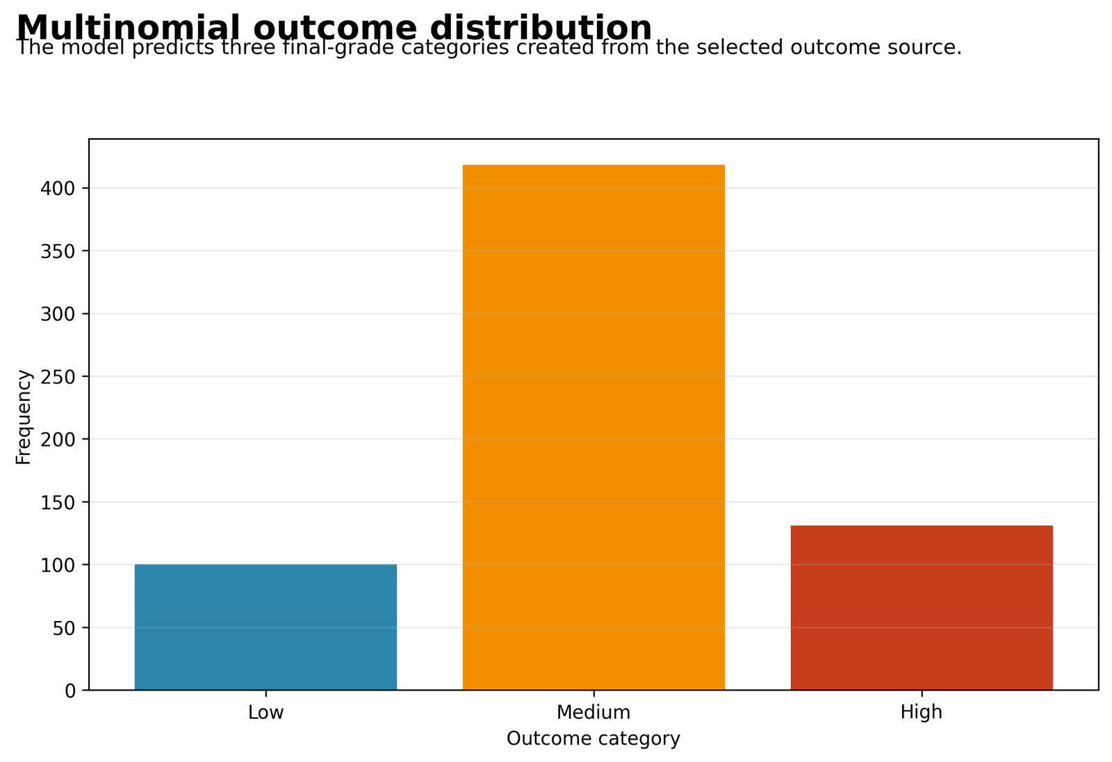
The bar chart shows the frequency of the three outcome classes created from G3. Medium is clearly the dominant category, High is much smaller and Low is the smallest nontrivial group.
Class counts are Low = 100 (15.41%), Medium = 418 (64.41%) and High = 131 (20.18%).
Most students end in the middle band rather than the extreme bands. That means the model gets much more information about what a medium final-grade profile looks like than about what a low-grade profile looks like. The class imbalance is not severe enough to invalidate the model, but it does make perfect Low-category classification harder than classifying the more common Medium category.
Report the class imbalance before interpreting accuracy. In Multinomial Logistic Regression, a high overall accuracy can partly reflect strong performance on the most common class, so class-by-class performance must also be shown.
Chart 2: Predicted Probability by Actual Class
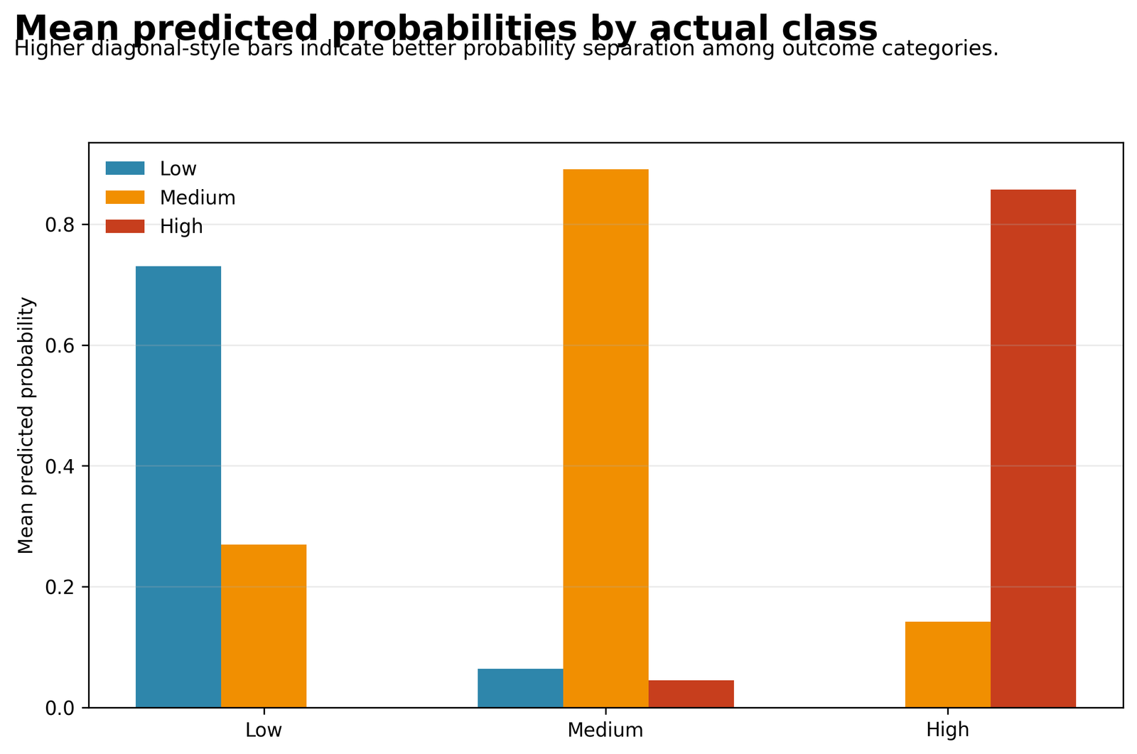
This figure compares the predicted class probabilities within each true class. Correctly classified observations tend to have larger probabilities for their actual class, while misclassified observations show more overlap with neighbouring classes.
The overall accuracy is 90.45% with 587 correct predictions out of 649. Low cases have the weakest recall (76.00%) and Medium cases the strongest recall (93.78%).
The model usually assigns the largest probability to the true class, but the certainty is not equally strong for every outcome. Medium and High students are recognized with high confidence more often than Low students, because Low cases sit closer to the Medium boundary and are more easily confused with it. The probability plot therefore reflects how separated the classes are in predictor space, not just whether the final label is right or wrong.
Use predicted probabilities in addition to hard class labels. A Multinomial Logistic Regression model is most useful when probability rankings are sensible, because those probabilities support risk targeting and threshold-based decisions.
Chart 3: Multinomial Confusion Matrix
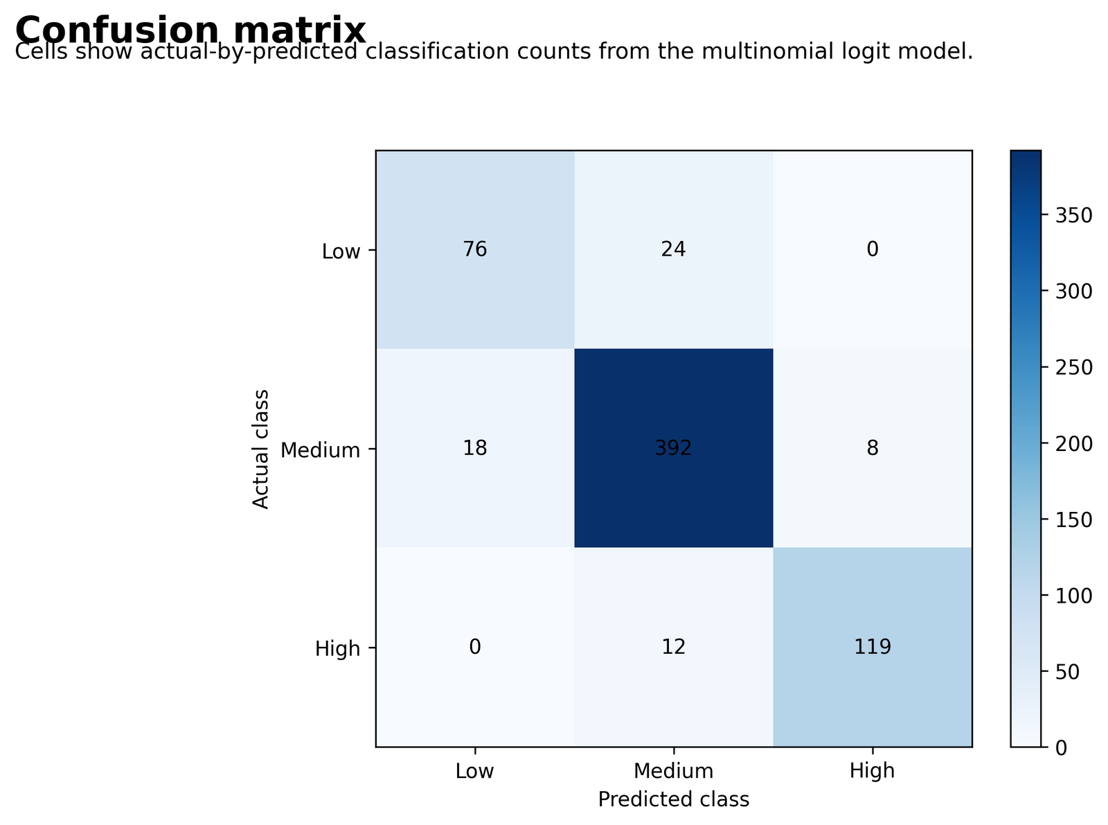
The heatmap places actual classes on one axis and predicted classes on the other. Large diagonal cells indicate correct classification and off-diagonal cells reveal where the model confuses neighbouring classes.
Correct classifications are 76 Low, 392 Medium and 119 High. Misclassifications are 24 Low→Medium, 18 Medium→Low, 8 Medium→High and 12 High→Medium. There are no Low→High or High→Low errors.
The model almost never mistakes the two extremes for each other. Instead, mistakes occur mainly at the boundaries around the Medium group. This means the predictors separate very weak performers from very strong performers reasonably well, but uncertainty appears when a student sits near the cut-points that define the Medium category. The Medium class acts as a transition band between the extremes.
Explain the error structure, not only the accuracy. In this Multinomial Logistic Regression model, boundary confusion is the main problem, so any practical intervention should focus on borderline Low/Medium and Medium/High cases.
Chart 4: Odds Ratios for Medium vs Low and High vs Low
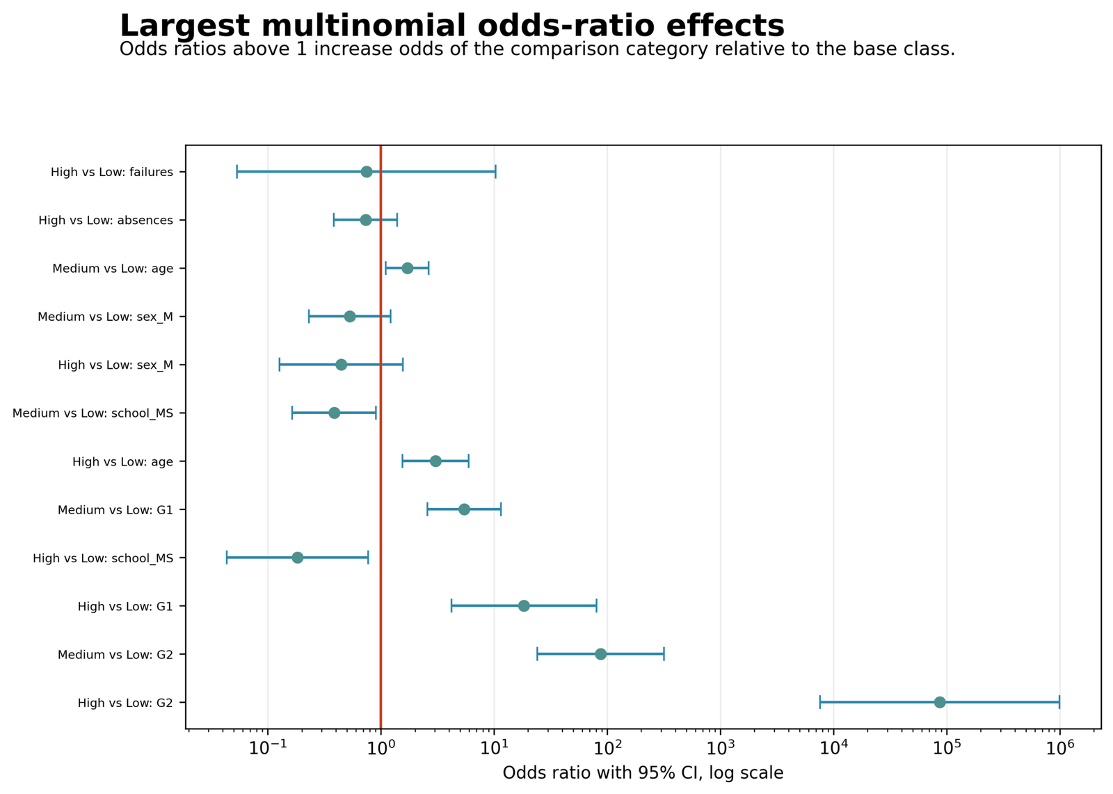
The coefficient plot compares exponentiated coefficients for each nonreference category against Low. Predictors with odds ratios above 1 increase the odds of that category relative to Low, while values below 1 reduce them.
For Medium vs Low, the strongest significant odds ratios are G2 = 87.60, G1 = 5.44, and age = 1.71, while school_MS = 0.39 is significantly below 1. For High vs Low, the supplied report clearly shows G1 = 18.37 as a strong positive contributor.
The model is telling a clear story: students with stronger earlier grades are far more likely to belong to the Medium or High G3 class than to the Low class. G2 is especially dominant because second-period performance is very close in time to the final outcome. Studytime and several demographic controls contribute far less once G1 and G2 are already in the model. In practice, academic history drives class membership much more than background covariates.
When reporting Multinomial Logistic Regression, separate the mathematically large odds ratios from the substantively important ones. Here, G1 and especially G2 are the practical drivers of category membership, while several other predictors add little independent information.
Chart 5: Predicted Class Distribution
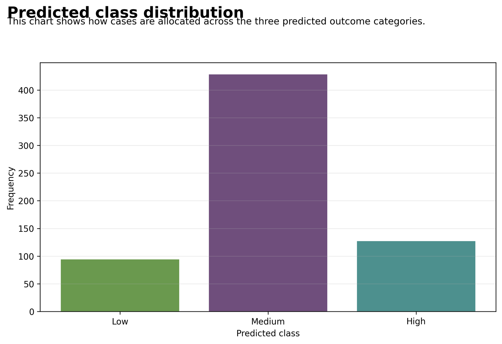
This chart compares how often the model predicts each category when all cases are classified to their most likely class.
Predicted counts are Low = 94 (14.48%), Medium = 428 (65.95%) and High = 127 (19.57%). These are very close to the observed counts of 100, 418 and 131.
The model is not wildly overproducing one class at the expense of the others. Its predicted class composition closely mirrors the true outcome distribution, which suggests the estimated probabilities are reasonably calibrated at the class level. That is important because a model can sometimes achieve decent accuracy while badly distorting class prevalence; that does not happen here.
Mention both observed and predicted class shares. A Multinomial Logistic Regression model is more trustworthy when it preserves the broad class composition as well as classifying individual observations well.
Chart 6: Probability of the High Category by Main Predictor
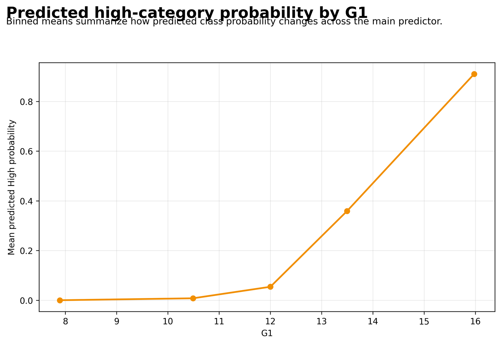
The figure tracks the predicted probability of the High class as the main academic predictor increases while other variables are held at representative values.
The report shows a strong High vs Low G1 coefficient = 2.9107, corresponding to an odds ratio of 18.37. Model-wide fit remains strong with McFadden pseudo R² = 0.7329 and χ² = 850.946.
As earlier performance improves, the chance of landing in the High final-grade band rises quickly rather than gradually. This is exactly what a strong multinomial model should show when prior academic performance meaningfully separates final outcome categories. In other words, the High class is not randomly assigned; it becomes much more probable for students already performing strongly before the final period.
Use this probability curve to communicate practical meaning. Instead of saying only that G1 is significant, explain that higher earlier grades move a student visibly toward the High final-grade category in the Multinomial Logistic Regression model.
Chart 7: Accuracy by Actual Class
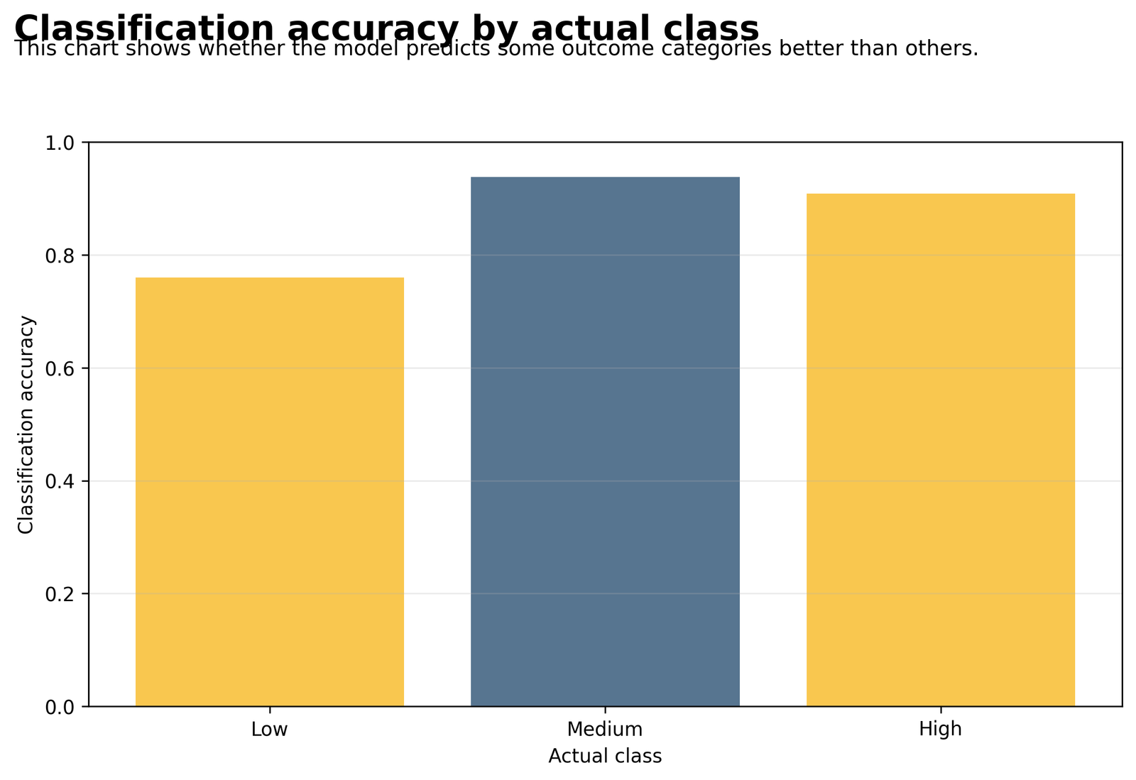
The chart compares class-specific recall across the three actual categories.
Class recall values are Low = 76.00%, Medium = 93.78% and High = 90.84%. Precision values are Low = 80.85%, Medium = 91.59% and High = 93.70%.
The model is excellent for Medium and High, but weaker for Low. That does not mean the Low class is unpredictable. It means Low cases are more likely to resemble lower-end Medium cases than to form a fully isolated cluster. The model therefore identifies most poor performers correctly, but it still misses about one-quarter of them by shifting them into Medium.
Always report per-class metrics in Multinomial Logistic Regression. A single overall accuracy of 90.45% looks strong, but the class-level results reveal that the Low category needs the most interpretive caution and perhaps targeted threshold tuning.
R Charts: Visual Validation of the Multinomial Logistic Regression Findings
The R images confirm the same underlying patterns found in Python: class imbalance, strong separation by prior grades, boundary-focused misclassification and high overall model performance.
R Outcome Distribution
The R outcome chart confirms that the Medium class dominates the sample, with Low and High much smaller. The important substantive point is that the model is being trained on an imbalanced but still usable three-class outcome, so classification quality must be evaluated per class rather than by overall accuracy alone.
R Predicted Class Distribution
The predicted-class distribution from R remains close to the observed class mix. That means the fitted model does not collapse toward the most frequent class and is reproducing class prevalence reasonably well at the population level.
R Confusion Matrix Heatmap
The R confusion matrix tells the same story as the Python matrix: nearly all errors occur between neighbouring categories, not between the two extremes. The model distinguishes very weak and very strong final outcomes fairly cleanly, while uncertainty is concentrated around the Medium boundary.
R Relative Risk Ratio Plot
The relative-risk-ratio plot in R highlights how strongly prior grades change the likelihood of higher outcome categories relative to Low. The key practical message is that earlier academic achievement is the dominant driver of class membership, whereas several controls contribute marginally once G1 and G2 are included.
R Predicted Probabilities by Case
The case-level probability display shows that many students receive a clearly dominant class probability, while a smaller set of boundary cases receive more mixed probability profiles. That means the Multinomial Logistic Regression model is making its biggest mistakes on cases that are genuinely ambiguous rather than on obviously well-separated profiles.
R Correct Versus Incorrect Probability
The correct-versus-incorrect probability chart shows that correctly classified cases generally have higher winning probabilities than incorrect cases. Errors happen primarily when the top two class probabilities are close, which is another sign of boundary uncertainty rather than global model failure.
R Class Performance Metrics
The class-performance metrics confirm that Medium and High have stronger recall/precision than Low. The practical takeaway is that the model is dependable overall, but decisions involving the Low class should consider class-specific uncertainty rather than relying only on the model-wide accuracy.
Key Coefficient Interpretation
Model-wide interpretation
The coefficients are log-odds effects for each nonreference class compared with Low. Exponentiating them yields odds ratios. In this Multinomial Logistic Regression model, the strongest effects come from earlier academic performance, especially G1 and G2.
Selected Medium versus Low results
| Predictor | Log-odds B | Odds ratio | 95% CI for OR | p | Meaning |
|---|---|---|---|---|---|
| G1 | 1.6935 | 5.4385 | 2.5664–11.5249 | <.001 | Higher G1 strongly increases the odds of Medium rather than Low |
| G2 | 4.4728 | 87.6037 | 24.1926–317.2211 | <.001 | Higher G2 overwhelmingly shifts students toward Medium rather than Low |
| age | 0.5352 | 1.7077 | 1.1075–2.6334 | .0154 | Older students are somewhat more likely to fall in Medium than Low after adjustment |
| school_MS | -0.9510 | 0.3864 | 0.1646–0.9067 | .0289 | School MS has lower odds of Medium vs Low than the reference school |
| studytime | 0.1425 | 1.1531 | 0.7419–1.7923 | .5266 | No clear independent Medium-vs-Low effect after adjustment |
Selected High versus Low results
| Predictor | Log-odds B | Odds ratio | p | Interpretation |
|---|---|---|---|---|
| G1 | 2.9107 | 18.3698 | .0001 | A one-unit increase in G1 greatly increases the odds of being High rather than Low |
| const | 0.7389 | 2.0937 | .5826 | The intercept is not statistically informative on its own |
Predicted Probabilities and Class Decisions
Observed class shares
- Low: 15.41%
- Medium: 64.41%
- High: 20.18%
Predicted class shares
- Low: 14.48%
- Medium: 65.95%
- High: 19.57%
For any individual case, Multinomial Logistic Regression produces three probabilities that sum to 1. The most likely class becomes the hard prediction, but the full probability vector still matters. A student predicted as Medium with probabilities 0.48, 0.45 and 0.07 is far less certain than a student predicted as Medium with probabilities 0.92, 0.06 and 0.02.
The confusion matrix shows that errors occur mainly because some students sit close to category cut-points rather than because the model fails globally. That is why the probability-based charts are so useful: they reveal how much certainty exists behind each class label.
Diagnostics and Assumptions
What to check
- Reference category coding
- Class counts and imbalance
- Multicollinearity among G1, G2 and other predictors
- Influential or boundary observations
- Probability separation and practical calibration
Main diagnostic message
- Model fit is strong
- Medium boundary cases drive most errors
- Low class needs the most caution
- Earlier grades dominate prediction
Key supporting diagnostics for Multinomial Logistic Regression include Variance Inflation Factor, Tolerance Statistic, Cook’s Distance, Influence Diagnostics and Outlier Detection. G1 and G2 are conceptually related, so coefficient instability should be checked even when classification performance is strong.
This model also carries the independence-of-irrelevant-alternatives assumption. If the categories behave as nested or partially substitutable choices, other models may sometimes be preferable. However, the supplied results suggest that the baseline-category approach works well for this educational outcome.
SPSS, Python, R and Excel Workflows
Python
Python estimated the supplied Multinomial Logistic Regression model and produced the main fit statistics, confusion matrix, predicted probabilities and seven charts.
- Likelihood-ratio χ² = 850.946
- McFadden pseudo R² = 0.7329
- Overall accuracy = 90.45%
R
R independently validates the same class structure and visual interpretation using the supplied chart set.
- Outcome and predicted-class distributions
- Confusion heatmap and relative-risk ratios
- Case-level probability diagnostics
SPSS
SPSS can fit Multinomial Logistic Regression through the NOMREG procedure with Low as the reference class and the same predictor set.
- Parameter estimates by class contrast
- Likelihood-ratio tests
- Pseudo R² and classification tables
Excel
The worked Excel file supports variable setup, interpretation and reporting. Excel can also be used to inspect predicted probabilities and confusion-matrix metrics once model coefficients are available.
- Outcome creation sheet
- Class counts and metrics
- Interpretation support
For additional software help, see correlation in Python, correlation in R, correlation in SPSS and correlation in Excel as general software-navigation companions.
Code: Expand Only the Software You Need
Python Multinomial Logistic Regression code
import pandas as pd
import statsmodels.api as sm

df = pd.read_csv("dataset.csv")
df["mlogit_grade_category"] = pd.cut(
    df["G3"],
    bins=[-1, 9, 14, 100],
    labels=["Low", "Medium", "High"]
)

X = df[["G1", "G2", "studytime", "failures", "absences", "age"]].copy()
X = pd.concat(
    [X, pd.get_dummies(df[["school", "sex", "address"]], drop_first=True)],
    axis=1
)
X = sm.add_constant(X)

y = df["mlogit_grade_category"]
model = sm.MNLogit(y, X).fit()
print(model.summary())
probs = model.predict(X)
R Multinomial Logistic Regression code
library(nnet)

df <- read.csv("dataset.csv")
df$mlogit_grade_category <- cut(
  df$G3,
  breaks = c(-Inf, 9, 14, Inf),
  labels = c("Low", "Medium", "High")
)
df$mlogit_grade_category <- relevel(df$mlogit_grade_category, ref = "Low")

fit <- multinom(
  mlogit_grade_category ~ G1 + G2 + studytime + failures +
    absences + age + school + sex + address,
  data = df,
  trace = FALSE
)
summary(fit)
probs <- predict(fit, type = "probs")
SPSS Multinomial Logistic Regression syntax
RECODE G3
 (Lowest thru 9=1)
 (10 thru 14=2)
 (15 thru Highest=3) INTO mlogit_grade_category.
VALUE LABELS mlogit_grade_category
 1 'Low' 2 'Medium' 3 'High'.

NOMREG mlogit_grade_category (BASE=FIRST)
 /CRITERIA CIN(95) DELTA(0) MXITER(100) MXSTEP(5)
 /MODEL G1 G2 studytime failures absences age
        school sex address
 /PRINT PARAMETER LRT CPS STEP MFI SUMMARY.
Excel workflow formulas and steps
Outcome category:
=IF(G3<10,"Low",IF(G3<15,"Medium","High"))

Observed class count:
=COUNTIF(category_range,"Low")

Predicted class:
=INDEX({"Low","Medium","High"},
 MATCH(MAX(prob_low,prob_med,prob_high),
       {prob_low,prob_med,prob_high},0))

Recall for Low:
=True_Low_Pred_Low / Actual_Low_Total

Precision for Low:
=True_Low_Pred_Low / Predicted_Low_Total
Advanced Interpretation and Extensions
What Multinomial Logistic Regression is
Multinomial Logistic Regression is a categorical-outcome model used when the dependent variable has more than two unordered categories. It extends Binary Logistic Regression by estimating separate logits for each nonreference class against a chosen base class.
When to use Multinomial Logistic Regression
Use Multinomial Logistic Regression when the outcome categories are nominal or when ordinal spacing is not assumed. If the categories have a strong ranking structure that should be modeled directly, compare this guide with Generalized Linear Model extensions and ordinal models.
Outcome coding and reference categories
The created outcome in this analysis uses G3 bands: Low < 10, Medium 10–14 and High ≥ 15. Low is the reference category. All other coefficients are interpreted relative to Low.
Log-odds versus odds ratios
Each coefficient is a change in log odds for one class relative to the reference class. Exponentiating the coefficient produces an odds ratio, which is easier to communicate because values above 1 indicate increased odds and values below 1 indicate decreased odds.
Relative risk ratios
Some software labels the exponentiated coefficient as a relative risk ratio. In practice, it is interpreted similarly to an odds ratio for baseline-category logits, but the term should match the software output that readers will see.
Baseline-category logit model
The baseline-category logit estimates one equation for Medium versus Low and another for High versus Low. The model therefore contains class-specific coefficients rather than one universal coefficient for every category.
Mathematical form of the model
Formally, the model estimates log[P(Y=j)/P(Y=Low)] = αj + βjX for each nonreference class j. The predicted probabilities across all classes must sum to 1 for every case.
Interpreting coefficients for each class
A coefficient can be significant for Medium versus Low but not for High versus Low, or vice versa. That is not a contradiction. It means the predictor has a different relationship with different category contrasts.
Why the reference class matters
The choice of reference class changes coefficient values and interpretations but not the underlying fitted probabilities. Choose a reference class that supports the clearest practical explanation.
Predicted probabilities
Predicted probabilities are often more useful than coefficients because they show the full class profile for a case. They also reveal whether the top prediction is highly confident or only marginally preferred.
Hard labels versus probabilities
A hard class label keeps only the largest predicted probability. That is convenient for classification tables, but it hides uncertainty. A student with probabilities 0.49, 0.48 and 0.03 is much less certain than a student with 0.92, 0.06 and 0.02.
Likelihood-ratio testing
The overall likelihood-ratio test compares the fitted model to a null model with no predictors. Here, χ² = 850.946, p < .001, so the predictors collectively improve class prediction strongly. See P-Value for significance interpretation.
Pseudo R-squared measures
McFadden pseudo R² is not interpreted like ordinary linear-model R². A value of 0.7329 is very strong for a discrete-choice model and indicates a major improvement over the null model, but it does not mean that 73.29% of outcome variance is explained in the linear-model sense.
AIC and BIC
AIC = 350.1674 and BIC = 439.6761 help compare competing models on the same data. Lower values indicate a better trade-off between fit and complexity. They are especially useful when comparing reduced and expanded predictor sets.
Confusion matrices
The confusion matrix shows not only how many predictions are correct but where the mistakes go. In this analysis, the model mostly confuses adjacent categories, which is substantively different from confusing the two extremes.
Class imbalance
Class imbalance affects how easily each category can be learned. The Medium class dominates the training sample, so its metrics are expected to be stronger than those of the smallest class unless the predictors separate all classes very cleanly.
Per-class precision and recall
Precision answers, “When the model predicts a class, how often is it correct?” Recall answers, “When a case truly belongs to that class, how often does the model recover it?” Multinomial Logistic Regression should report both.
Overall accuracy versus balanced performance
Overall accuracy summarizes the total proportion correct, but balanced evaluation asks whether each class is being served adequately. A model can look good overall while still missing too many cases in a smaller but important class.
Independence of irrelevant alternatives
The independence-of-irrelevant-alternatives assumption states that odds between two classes are unaffected by the presence or properties of another class. When this is implausible, nested or mixed models may be preferable.
Multicollinearity
Check Variance Inflation Factor and Tolerance Statistic for continuous predictors. In educational data, G1 and G2 can be highly correlated, so coefficient instability should be examined even when prediction is strong.
Influential observations
Use Cook’s Distance, leverage and Influence Diagnostics to detect observations that disproportionately affect class-separation estimates. Borderline cases near category cut-points often deserve special inspection.
Linearity in the logit for continuous predictors
Continuous predictors should have approximately linear effects in the logit for each contrast. If not, splines, category recoding or a flexible model may fit better.
Alternative models
Alternative models include Logistic Regression for two classes, Generalized Estimating Equations for clustered outcomes, Generalized Additive Model for nonlinear effects and Bayesian Regression when prior structure is important.
Ordinal versus multinomial logistic regression
If the outcome truly follows an order, ordinal logistic regression may be more parsimonious than Multinomial Logistic Regression. In this analysis the grade bands are ordered, but the multinomial approach was used to allow class-specific effects without imposing a proportional-odds constraint.
Power and sample size
Power depends on the number of classes, the size of the smallest class and the strength of separation. Use Statistical Power planning and avoid focusing only on total sample size.
APA-style reporting decisions
For publication, report the reference class, all predictor sets, model-fit statistics, class counts, confusion matrix, class-level metrics and key odds ratios with confidence intervals. That produces a transparent Multinomial Logistic Regression write-up.
APA-Style Reporting
For Medium versus Low, G1 (OR = 5.44, 95% CI [2.57, 11.52], p < .001) and G2 (OR = 87.60, 95% CI [24.19, 317.22], p < .001) were strong positive predictors. For High versus Low, G1 was also strongly positive (OR = 18.37, p = .0001). Class-specific recall was 76.00% for Low, 93.78% for Medium and 90.84% for High.
When reporting Multinomial Logistic Regression, always specify the reference category, report class counts and explain what the predicted probabilities mean in practice. Use exact p-values and confidence intervals whenever they are available.
Publication Checklist and Common Mistakes
Include in the final report
- Definition of the three outcome classes
- Reference category
- All predictors and coding
- Likelihood-ratio test and pseudo R²
- Confusion matrix and class metrics
- Key odds ratios with confidence intervals
- Predicted probability interpretation
Avoid these errors
- Reporting only overall accuracy
- Ignoring class imbalance
- Forgetting the reference category
- Treating pseudo R² like linear-model R²
- Explaining coefficients without a practical probability story
- Assuming category boundaries are irrelevant
Before publication, revisit Null and Alternative Hypothesis, Type I and Type II Error and Statistical Power to frame uncertainty responsibly in your Multinomial Logistic Regression discussion.
Downloads
Frequently Asked Questions
What is Multinomial Logistic Regression?
When should Multinomial Logistic Regression be used?
What is the dependent variable in this analysis?
What is the reference category?
How many cases were analyzed?
Was the overall model significant?
What is the pseudo R-squared?
What is the overall classification accuracy?
Which class is hardest to classify?
Which class is easiest to classify?
What do odds ratios above 1 mean?
What does an odds ratio below 1 mean?
Why should predicted probabilities be reported?
Is Multinomial Logistic Regression the same as ordinal logistic regression?
Can Multinomial Logistic Regression prove causation?
How should Multinomial Logistic Regression be reported?
Final Multinomial Logistic Regression Conclusion
This Multinomial Logistic Regression model fits strongly and classifies the three G3 categories with high overall success. The model shows that prior grades—especially G1 and G2—are the main drivers of whether a student falls into the Low, Medium or High final-grade class.
The mistakes are informative: the model rarely confuses the two extremes with each other and instead makes most of its errors at the Medium boundaries. That means the main practical challenge is distinguishing borderline cases rather than separating very low-performing from very high-performing students.

