
Siegel Tukey Test: 7 Essential Steps, Formula and Worked Example
The Siegel Tukey Test is a nonparametric two-sample dispersion procedure that ranks observations by alternating between the pooled extremes and the center. This complete guide explains the Siegel Tukey Test assumptions, median adjustment, alternating-extreme score construction, tie handling, interpretation, and reproducible workflows in Python, R, SPSS, Excel, MATLAB and SAS.
No statistically significant difference in median-adjusted grade dispersion was detected.
In this worked Siegel Tukey Test example, final grades were compared between female students (n = 383) and male students (n = 266). The original group medians were 12 and 11, so each observation was centered on its own group median before the scale test. The verified female score sum was T = 121,481.971071, compared with an expected value of 124,475. The standardized result was z = -1.303626 with a two-sided p = 0.192361. At α = .05, equal median-adjusted dispersion was not rejected.
What does the Siegel Tukey Test measure?
A rank-based comparison of relative spread for two independent samples.
The Siegel Tukey Test evaluates whether two independent populations differ in scale or dispersion after location has been made comparable. It is not Tukey HSD, not a post-hoc ANOVA procedure and not a generic test of any distributional difference. The Siegel Tukey Test uses a distinctive alternating-extreme ranking scheme so observations far from the pooled center receive the smallest scores.
The research question
The test addresses a focused question: after allowing for location, does one group occupy the pooled extremes more often than the other? A group with a larger population scale should contribute more observations to both tails. Since the Siegel–Tukey scoring rule assigns low scores to extreme positions and high scores near the pooled center, a group that is more dispersed tends to have a smaller total score.
This makes the procedure useful for response times, grades, manufacturing measurements, clinical outcomes and other ordered variables where the investigator cares about variability rather than a shift in the center. Review variance, standard deviation and the interquartile range before interpreting a formal scale comparison.
What it does not measure
The Siegel Tukey Test does not directly test means, medians, stochastic dominance or all possible shape differences. A significant result can be interpreted as a scale difference only when the groups have a common location or a justified location adjustment has been performed. If the scientific question concerns general rank location, use the Mann–Whitney U test. If the objective is complete distributional equality, consider the two-sample Kolmogorov–Smirnov test.
The method is also unrelated to Tukey’s honestly significant difference test. Tukey HSD compares means after ANOVA; the Siegel Tukey Test is a two-sample nonparametric dispersion test developed around alternating-extreme ranks.
When should you use the Siegel Tukey Test?
Use the decision logic below before selecting software.
Use the Siegel Tukey Test when there are exactly two independent groups, the outcome is orderable, the research target is dispersion and location has either been shown to be common or has been adjusted in a defensible way. A failed normality test alone is not enough justification.
Two groups?
The standard procedure compares exactly two independent samples.
Ordered outcome?
The response must be numeric or ordinal with a meaningful low-to-high order.
Independent units?
No student, patient, device or cluster should appear in both groups.
Comparable location?
Check medians before interpreting alternating-extreme ranks as scale.
Scale question?
The hypothesis must concern dispersion rather than mean or median differences.
Good uses
Do not use it automatically
The current example illustrates why the location check cannot be skipped. Female students have an observed median final grade of 12, while male students have a median of 11. Applying the ordinary unadjusted procedure to those raw values would mix location and scale. The workbook therefore centers grades within gender before assigning the alternating-extreme scores. That choice changes the precise inferential target: the result concerns spread around the separately estimated group medians.
Siegel Tukey Test assumptions: six conditions to check
The method is nonparametric, but it is not assumption-free.
The Siegel Tukey Test assumptions determine whether a rank-sum result can be interpreted as evidence about scale. Independence, an orderable outcome, comparable location, similar standardized shape, transparent handling of ties and a design supporting inference are substantive conditions.
Independent samples
Observations must be independent within and between groups. Clustered, matched or repeated measurements need a design-aware alternative.
Ordered outcome
The response must support meaningful ranking. Continuous outcomes are ideal, but tied integer outcomes can be analyzed with averaged scores.
Comparable location
A pure scale interpretation requires a common population center or a justified adjustment for a location difference.
Comparable shape
The cleanest interpretation assumes the populations share a similar standardized shape apart from scale.
Random design
Random sampling or random assignment is needed for broad population or causal inference.
Ties handled explicitly
Tied centered values share the average of all alternating-extreme scores associated with their occupied positions.
Nonparametric procedures still require careful design reasoning. See parametric vs nonparametric tests for a broader explanation. The most important question is not whether the data are normal; it is whether alternating-extreme ranks answer the scientific question you actually have.
Siegel Tukey Test hypotheses: population scale after location adjustment
State the scale null and identify the centered outcome used in the analysis.
The Siegel Tukey Test does not literally test whether the observed standard deviations are numerically equal. It tests whether two independent population distributions have equal relative spread under the model and alignment used to construct the alternating-extreme scores.
Formal location–scale idea
For a clean unadjusted interpretation, the two populations can be represented as sharing a location θ and standardized shape ε while allowing different positive scale multipliers:
If θ differs, pooled extremes can be created by a location shift rather than a scale difference. The current analysis therefore replaces raw grades with deviations from the observed gender-specific medians.
Applied variables
The public article uses the label gender consistently. The categories F and M are treated as the two independent groups supplied in the analysis files.
Two-sided test
Applied wording: after median adjustment, the female and male population distributions have equal spread under the assumed common standardized shape.
Directional alternatives
A smaller-than-expected female score sum supports greater female spread.
A larger-than-expected female score sum supports smaller female spread.
Either direction can produce rejection.
Choose a directional alternative before seeing the scores. The current article uses the safer two-sided alternative.
What the observed score sum says
The observed female score sum was 121,481.971071, below its null expectation of 124,475. Since low scores are assigned to pooled extremes, the sign points toward somewhat greater female tail occupancy after centering. However, the standardized distance is only z = -1.304 and the two-sided p-value is 0.192. The directional hint is not statistically significant and should not be converted into a firm population conclusion.
Siegel Tukey Test formula, alternating-extreme scores and large-sample calculation
The test orders the pooled centered values and scores them from the extremes toward the center.
The Siegel Tukey Test formula can be understood as a Wilcoxon-style rank-sum test applied to a special score sequence. Unlike ordinary ranks, the scores alternate between the lowest and highest pooled positions so extreme observations receive small numbers and central observations receive large numbers.
Step 1: center when location differs
The current workbook subtracts each gender group’s sample median. Female grades are centered on 12 and male grades on 11.
Step 2: pool and sort the centered values
Combine all 649 centered observations and order them from the smallest negative deviation to the largest positive deviation. At this stage, group labels remain attached to the observations but do not affect score assignment.
Step 3: assign alternating-extreme scores
| Assignment step | Pooled position | Score | Interpretation |
|---|---|---|---|
| 1 | Smallest centered value | 1 | Extreme low tail |
| 2 | Largest centered value | 2 | Extreme high tail |
| 3 | Second largest | 3 | Next high-tail position |
| 4 | Second smallest | 4 | Next low-tail position |
| 5 | Third smallest | 5 | Continue inward |
| 6 | Third largest | 6 | Continue inward |
T is the sum of tie-adjusted Siegel–Tukey scores for the female sample. Small T values place more female observations at the pooled extremes.
The score vector is a permutation of 1 through N before tie averaging, so s̄ = (N + 1)/2 = 325. Therefore E(T) = 383 × 325 = 124,475.
The workbook evaluates this finite-population variance from the complete tie-adjusted score set.
The two-sided large-sample p-value is calculated from |z| using the standard normal distribution.
Verified large-sample calculation
Direction of the result
The female score sum is 2,993.029 points below expectation. Since extremes receive low scores, the sign is consistent with slightly greater female spread after median centering. The evidence is not strong enough to reject equal scale.
The standardized descriptive index |z|/√N is 0.051. This is small and should be reported only as a descriptive supplement, not as a universally standardized Siegel–Tukey effect size.
Siegel Tukey Test example: final-grade dispersion by gender
A complete worked comparison using 649 final grades.
This Siegel Tukey Test example uses the final grade G3 and a two-level gender grouping. It documents the original location difference, median centering, alternating-extreme scores, tie averaging, group score sum, expected value, variance, z statistic and final interpretation.
Research scenario
The outcome is final grade G3. The research question asks whether grade dispersion around the group-specific median differs between female and male students. The original medians are not identical, so the workbook subtracts each group’s observed median before pooling the deviations.
This wording is more accurate than saying the raw distributions have equal location. It also prevents the scale conclusion from being confused with the observed one-point median difference.
Variables used
| Role | Variable | Coding / meaning |
|---|---|---|
| Outcome | G3 | Final numeric grade, observed from 0 to 19. |
| Grouping | Gender | F = female; M = male. |
| Sample 1 | F | n = 383. |
| Sample 2 | M | n = 266. |
| Analyzed score input | Centered G3 | Raw grade minus the within-gender median. |
Siegel Tukey Test statistics, results and interpretation
All verified outputs reconcile to the same nonsignificant conclusion.
The Siegel Tukey Test statistics connect the female score sum to the null distribution. The observed score sum is below expectation, but only 1.304 standard errors away, so the two-sided result does not reject equal median-adjusted dispersion.
Primary inference
Fail to reject H0
At α = .05, the data do not provide statistically significant evidence that centered final-grade dispersion differs between female and male students.
Calculation audit
| Evidence | Verified value | Decision | Interpretation |
|---|---|---|---|
| Female score sum | 121,481.971071 | Below expectation | Directional tendency toward more female extreme occupancy |
| Expected score sum | 124,475 | Null reference | Based on random labels and the complete score set |
| z statistic | -1.303626 | Not extreme | Only 1.304 standard errors below expectation |
| Two-sided p-value | 0.192361246 | Fail to reject | No significant scale difference detected |
Siegel Tukey Test in Python: complete calculation and charts
A transparent custom calculation reproduces the workbook exactly.
The Siegel Tukey Test in Python should expose the location adjustment, alternating-extreme score sequence, tie averaging and finite-population variance. A generic rank-sum function is not enough unless the special Siegel–Tukey scores have already been constructed correctly.
import numpy as np
import pandas as pd
from scipy.stats import norm# The public analysis label is gender; categories are F and M.
df = pd.read_csv("student_grades.csv")[["G3", "gender"]].dropna()
# Align locations separately because the original medians are 12 and 11.
df["centered_G3"] = df["G3"] - df.groupby("gender")["G3"].transform("median")
df = df.sort_values("centered_G3", kind="mergesort").reset_index(drop=True)
N = len(df)
# Raw Siegel-Tukey position scores: lowest, highest, second-highest,
# second-lowest, then repeat the same two-from-each-extreme pattern.
pos_score = np.empty(N, dtype=float)
left, right, s = 0, N - 1, 1
while left <= right:
pos_score[left] = s; left += 1; s += 1
if left <= right:
pos_score[right] = s; right -= 1; s += 1
if left <= right:
pos_score[right] = s; right -= 1; s += 1
if left <= right:
pos_score[left] = s; left += 1; s += 1
# Average occupied position scores inside every tied centered value.
df["position_score"] = pos_score
df["st_score"] = df.groupby("centered_G3")["position_score"].transform("mean")
focus = "F"
n1 = (df["gender"] == focus).sum()
n2 = N - n1
T = df.loc[df["gender"] == focus, "st_score"].sum()
a = df["st_score"].to_numpy()
a_bar = a.mean()
E = n1 * a_bar
V = (n1 * n2 / (N * (N - 1))) * np.sum((a - a_bar) ** 2)
z = (T - E) / np.sqrt(V)
p_value = 2 * norm.sf(abs(z))
print(T, E, V, z, p_value)
Python result summary
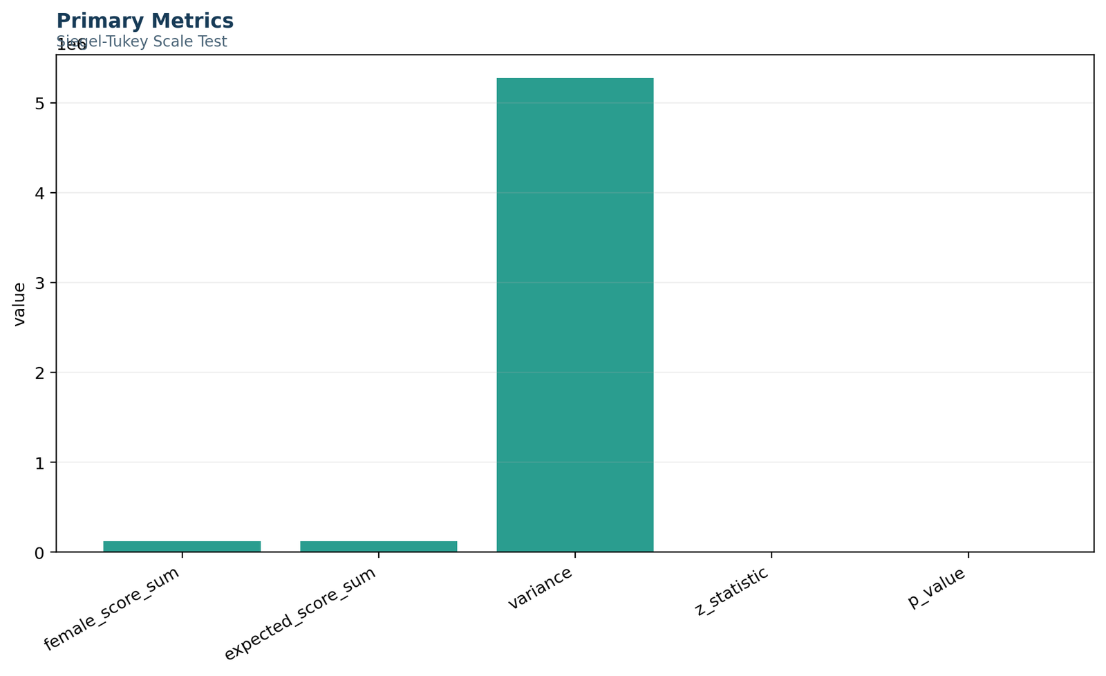
The first Python chart gives the complete statistical headline: female n = 383, male n = 266, female score sum = 121,481.971, expected score sum = 124,475, variance = 5,271,279.283, z = -1.304 and p = 0.192. It is full-width so the compact metrics remain readable.
Python gender scale summary
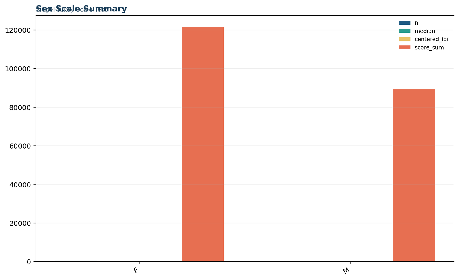
The group summary combines sample size, original median, centered spread summaries and score totals. The chart retains the supplied F and M coding while the article uses the public label gender. The important pattern is that descriptive spread measures are close and the female score sum is only modestly below expectation.
Python alternating-extreme scores
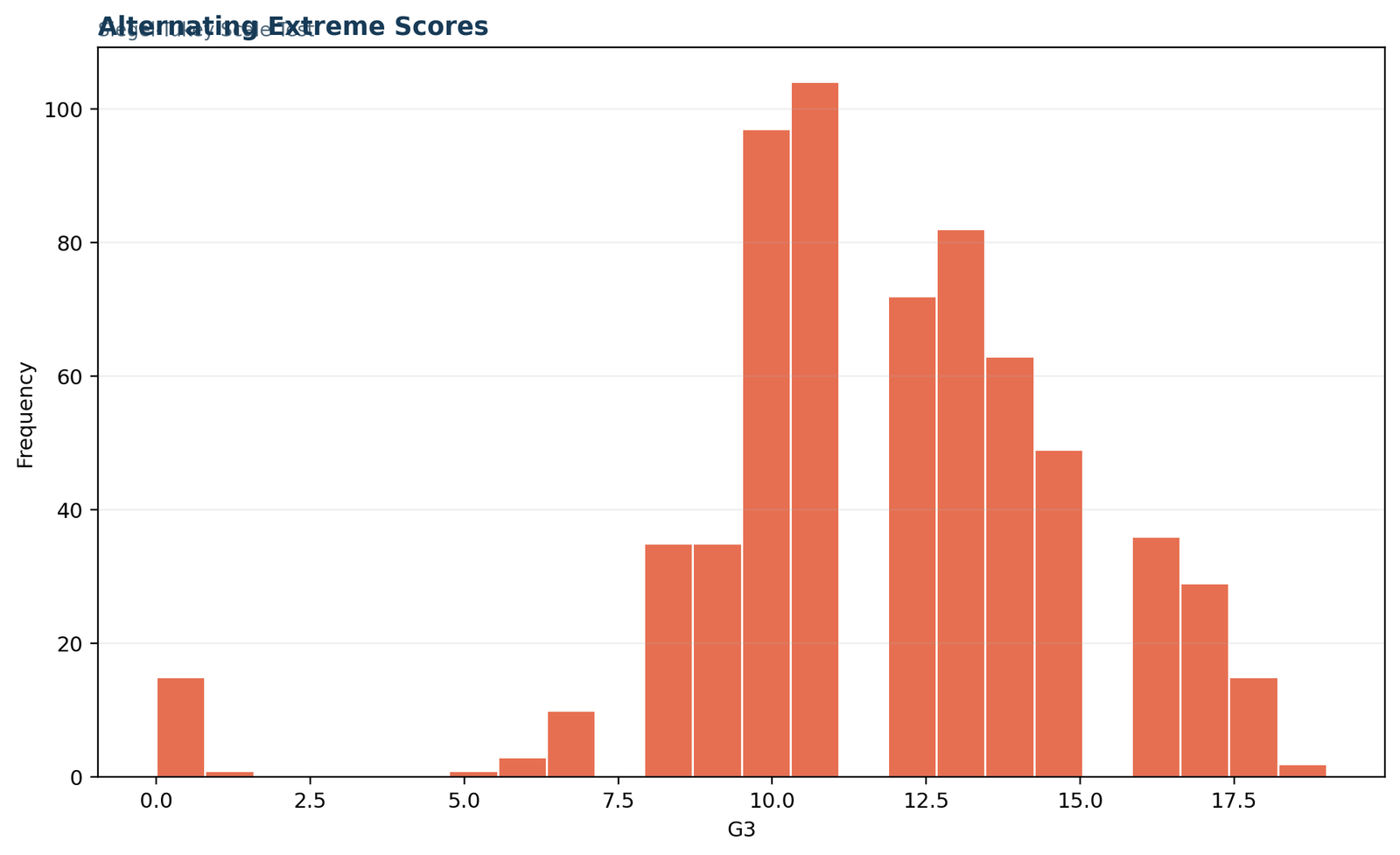
This method-specific chart shows the centered grade values and the way scores rise toward the pooled center. Very low and very high centered grades receive small scores, while values near zero receive the largest scores. The pattern explains why a more dispersed group tends to produce a smaller score sum.
Python score quantiles
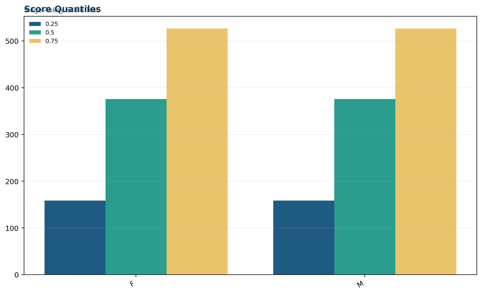
The female and male score quantiles are almost identical: the pooled score quartiles are approximately 158.5, 375.493 and 526.5. The similarity of the central score summaries supports the nonsignificant result.
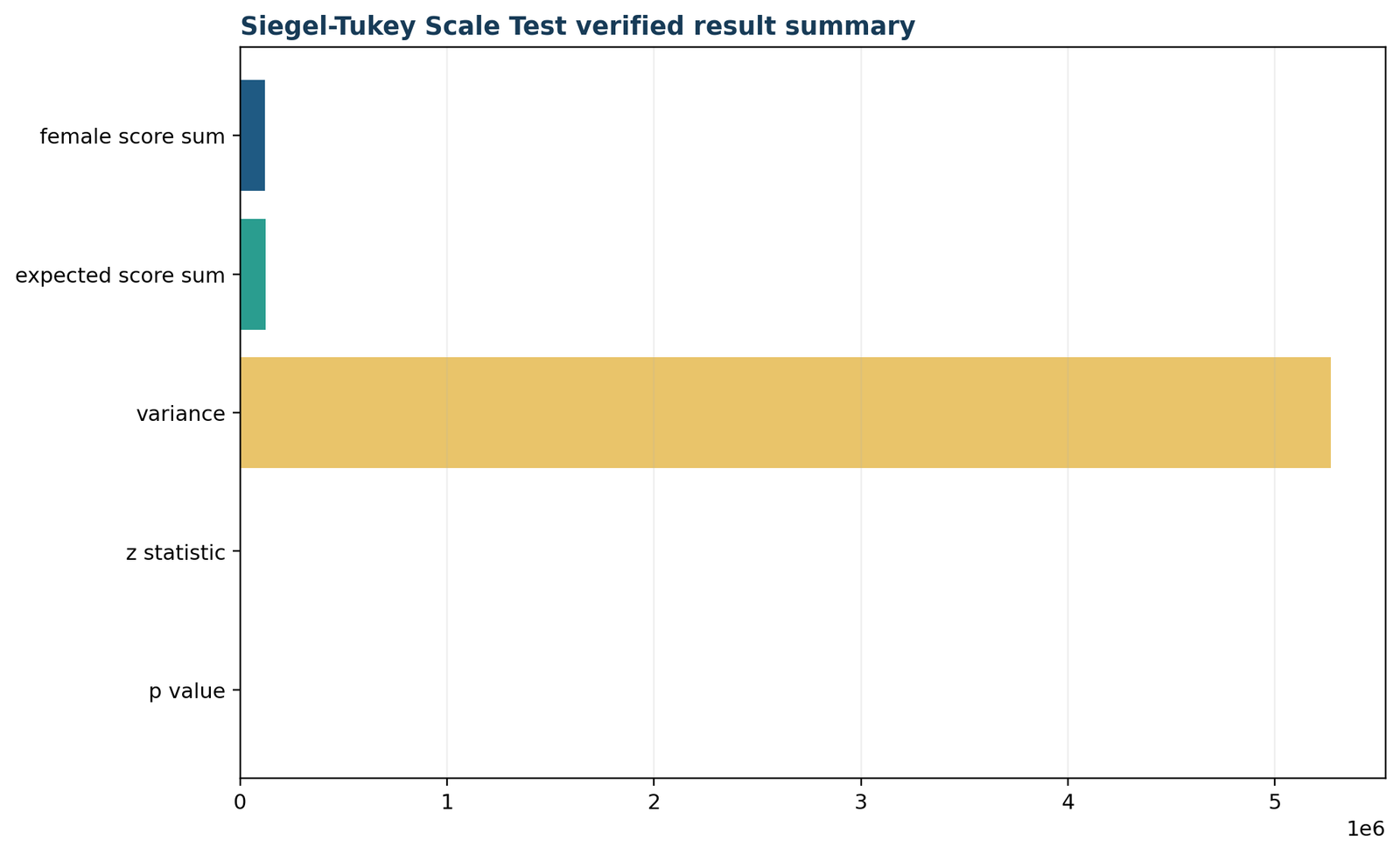
Python verified result summary
The final Python panel consolidates the observed sum, expected sum, variance, z statistic and p-value. Agreement with the workbook confirms that the location alignment, alternating-extreme sequence, tie correction and random-label variance were implemented consistently.
Siegel Tukey Test in R: reproducible scores, ties and validation
The R section uses exactly the same chart layout and statistical target as Python.
The Siegel Tukey Test in R can be run through a specialist package or implemented transparently with custom scores. The custom workflow shown here is useful because it makes the sample-median alignment and tie-adjusted score construction visible rather than relying on undocumented defaults.
library(dplyr)df <- read.csv("student_grades.csv") |>
select(G3, gender) |>
filter(complete.cases(.)) |>
group_by(gender) |>
mutate(centered_G3 = G3 - median(G3)) |>
ungroup() |>
arrange(centered_G3)
N <- nrow(df)
position_score <- rep(NA_real_, N)
left <- 1; right <- N; s <- 1
while (left <= right) {
position_score[left] <- s; left <- left + 1; s <- s + 1
if (left <= right) {position_score[right] <- s; right <- right - 1; s <- s + 1}
if (left <= right) {position_score[right] <- s; right <- right - 1; s <- s + 1}
if (left <= right) {position_score[left] <- s; left <- left + 1; s <- s + 1}
}
df$position_score <- position_score
df <- df |>
group_by(centered_G3) |>
mutate(st_score = mean(position_score)) |>
ungroup()
n1 <- sum(df$gender == "F")
n2 <- N - n1
T <- sum(df$st_score[df$gender == "F"])
a_bar <- mean(df$st_score)
E <- n1 * a_bar
V <- (n1 * n2 / (N * (N - 1))) * sum((df$st_score - a_bar)^2)
z <- (T - E) / sqrt(V)
p_value <- 2 * pnorm(-abs(z))
c(T=T, expected=E, variance=V, z=z, p=p_value)
Specialist R packages also provide Siegel–Tukey functions, but package defaults can differ on median adjustment, exact inference, score direction and tie handling. The article therefore reports the audited custom calculation and uses package output only as a secondary cross-check. The verified R result matches Python and Excel to floating-point precision.
R result summary
The R result summary reproduces the same verified metrics as Python. It uses the same full-width card placement, not a smaller layout, so the statistical labels and scaled bars remain readable on desktop.
R gender scale summary
This R chart mirrors the Python gender summary in the same two-column card width. It shows the sample-size imbalance, the original medians, centered spread summaries and group score totals without changing the underlying analysis.
R alternating-extreme scores
The R score profile shows the same alternating-extreme logic as Python. Scores are smallest in both tails and largest near centered zero, demonstrating that the method measures relative spread rather than location.
R score quantiles
The R score quantile panel matches the Python panel in size, order and caption structure. The nearly overlapping quantiles are consistent with the failure to reject equal median-adjusted scale.
R verified result summary
The final R panel repeats the audited statistic and p-value. Numerical agreement across R, Python and Excel is the central reproducibility check for this tied, median-adjusted analysis.
Siegel Tukey Test SPSS workflow and corrected interpretation
SPSS supports the data preparation, but the score test requires a custom workflow.
A Siegel Tukey Test SPSS analysis requires care because the standard menus do not expose a dedicated alternating-extreme score dialog. The supplied SPSS output should therefore be described as a validated custom workflow rather than as a native one-click table.
What SPSS can do directly
SPSS can verify coding, missing values, group sizes, medians, standard deviations, quartiles, histograms and boxplots. It can also calculate group medians, create centered grades and preserve the full row-level audit trail. These steps are essential because the original medians differ.
The final alternating-extreme score assignment and tie-adjusted variance can be completed through syntax, Python/R integration or an imported score column generated from the verified workbook.
Recommended workflow
* Rename the source grouping field to gender for public reporting.
RENAME VARIABLES (sex = gender).* Center G3 within each gender group before the scale comparison.
AGGREGATE OUTFILE=* MODE=ADDVARIABLES
/BREAK=gender
/group_median=MEDIAN(G3).
COMPUTE centered_G3=G3-group_median.
EXECUTE.
* SPSS has no standard one-click Siegel-Tukey dialog.
* Sort pooled centered values, assign alternating-extreme scores,
* average score positions within ties, and calculate the group sum,
* expectation, finite-population variance, z, and two-sided p.
* The supplied PDF documents the validated custom workflow.
Siegel Tukey Test Excel calculation with median adjustment and ties
The worked workbook provides a full row-level audit trail.
The Siegel Tukey Test Excel file separates raw data, centered values, test scores, calculations, diagnostics and verified reporting. It is designed to show every numerical step rather than presenting a decorative p-value.
Recommended worksheet process
1. Calculate each group median and centered value:

=G3 - MEDIANIFS(G3_range, gender_range, current_gender)

2. Sort all centered values together from smallest to largest.

3. Assign raw Siegel-Tukey scores in this order:

lowest=1, highest=2, second-highest=3, second-lowest=4,

third-lowest=5, third-highest=6, fourth-highest=7,

fourth-lowest=8, and continue.

4. Average the occupied position scores inside ties with AVERAGEIFS.

5. Female score sum:

=SUMIFS(score_range, gender_range, "F")

6. Expected sum:

=nF*AVERAGE(score_range)

7. Variance:

=nF*nM/(N*(N-1))*DEVSQ(score_range)

8. z and p:

=(T-E)/SQRT(V)

=2*(1-NORM.S.DIST(ABS(z),TRUE))The reporting sheet cross-checks the workbook values against an independently verified reference. The differences are only floating-point rounding: approximately 1.46 × 10⁻¹¹ for the score sum and 3.26 × 10⁻¹⁴ for the p-value. This confirms that Excel reproduces the intended calculation accurately.
Siegel Tukey Test in MATLAB and SAS
SAS provides native Siegel–Tukey scores; MATLAB generally requires a custom score routine.
Searches for the Siegel Tukey Test MATLAB and Siegel Tukey Test SAS often lead to Tukey HSD material instead. The procedures are unrelated. SAS PROC NPAR1WAY provides the ST option, while MATLAB users can reproduce the alternating-extreme ranks directly.
MATLAB custom implementation
% G3 and gender are column vectors.

centered = G3;

centered(gender=="F") = G3(gender=="F") - median(G3(gender=="F"));

centered(gender=="M") = G3(gender=="M") - median(G3(gender=="M"));

% Sort pooled centered values, create the alternating-extreme

% position scores, average within ties, then calculate T, E, V, z and p.
MATLAB does not need a dedicated function for the calculation because the score sequence is deterministic. The implementation should be checked against the verified values in this guide.
SAS PROC NPAR1WAY
proc npar1way data=centered_grades st;

class gender;

var centered_G3;

exact st / mc;

run;
The ST option requests Siegel–Tukey scores. SAS documentation notes that the procedure can provide asymptotic and exact or Monte Carlo inference. Report whether continuity correction, exact calculation or Monte Carlo estimation was used, because those details can produce small differences from the workbook’s uncorrected normal calculation.
Siegel Tukey Test vs Ansari Bradley, Levene and other scale tests
Choose according to the design, score system and inferential target.
The Siegel Tukey Test vs Ansari Bradley Test comparison is especially important because both are two-sample nonparametric scale procedures. They differ in their score patterns: Siegel–Tukey alternates ranks from the extremes, while Ansari–Bradley assigns directly symmetric center-outward scores.
| Method | Main target | Core mechanism | Location concern | Best use |
|---|---|---|---|---|
| Siegel–Tukey | Two-sample relative spread | Alternating-extreme ranks | Requires comparable location or justified alignment | Ordinal or numeric independent samples |
| Ansari–Bradley | Two-sample scale | Symmetric center-outward scores | Common location is central | Classical rank-based scale comparison |
| Levene test | Equality of dispersion | ANOVA on absolute deviations | Uses a chosen center | Widely used for two or more groups |
| Brown–Forsythe test | Robust equality of dispersion | Absolute deviations from group medians | Median-centered by design | Robust multi-group comparison |
| Fligner–Killeen test | Homogeneity of scale | Ranked absolute deviations | Robust center handling | Three or more groups or robust sensitivity |
| Moses test | Extreme reaction spread | Control-span logic | Different construction | Extreme-dispersion alternatives |
The current result can be compared with descriptive and alternative scale methods as a sensitivity analysis. However, analysts should not run many scale tests and report only the smallest p-value. Select a primary method before seeing the results and use alternatives to assess robustness, not to search for significance.
Why alternating-extreme ranks answer a different question
The Siegel Tukey Test is often introduced as if it were simply a Wilcoxon test with an unusual ranking order. That description is mechanically true but scientifically incomplete. Ordinary ranks increase monotonically from the smallest to the largest observation, so their sum is sensitive primarily to location or stochastic ordering. Siegel–Tukey scores deliberately break that monotonic pattern. They assign small values at both ends and large values near the middle. As a result, the Siegel Tukey Test reacts when one group occupies both tails more often, which is the pattern expected from a larger scale after location has been aligned.
This distinction also explains why the sign of the score difference can seem counterintuitive. In the current Siegel Tukey Test, the female sum is below its expectation. A lower score sum does not mean lower grades; it means more observations have received the low numbers reserved for pooled extremes. Because the grades were centered first, those extremes represent unusually large negative or positive deviations from the gender-specific median. Direction should therefore be described in terms of relative spread, not academic performance.
What the nonsignificant result does and does not imply
A p-value of 0.192 means the observed score imbalance is compatible with ordinary random variation under the equal-scale reference model. The Siegel Tukey Test did not detect a statistically persuasive difference, but the result does not establish exact equality. There may be a small population-scale difference that the current data and score test cannot distinguish from sampling noise. The standardized index of 0.051 is consistent with a small departure, and the centered absolute deviations are almost identical. Together, those pieces of evidence support a restrained conclusion rather than an absolute statement.
Formal equivalence requires a different design. Researchers would need to define a practically negligible range for a scale ratio or another dispersion parameter and then demonstrate that uncertainty lies inside that range. The Siegel Tukey Test provides a conventional difference test, so its nonsignificant outcome should be reported as insufficient evidence against equal median-adjusted scale.
Eight interpretation questions to answer before publication
Was the Siegel Tukey Test chosen because dispersion was the primary estimand? Was the Siegel Tukey Test applied to independent samples? Did the Siegel Tukey Test use an outcome with a meaningful order? Was location checked before the Siegel Tukey Test scores were assigned? Were ties in the Siegel Tukey Test averaged across all occupied positions? Does the reported Siegel Tukey Test statistic belong to a clearly named focus group? Is the Siegel Tukey Test p-value linked to the stated asymptotic, exact or Monte Carlo method? Does the final Siegel Tukey Test conclusion avoid claiming proven equality?
Answering all eight questions creates a compact audit trail. In the present analysis, the design is independent, the outcome is ordered, the original medians are disclosed, separate-median centering is stated, ties are averaged, the female group is the focus, the normal reference calculation is identified and the conclusion is deliberately cautious. The Siegel Tukey Test is therefore reproducible from the supplied files, and the Siegel Tukey Test interpretation remains tied to the stated median-adjusted target.
Diagnostics, sensitivity checks and common mistakes
A defensible analysis combines the p-value with location, shape and tie checks.
A credible Siegel Tukey Test report must explain why the score sum represents dispersion rather than location. Diagnostics should examine medians, standardized shapes, ties, bounded outcomes, influential tails, group imbalance and sensitivity to the chosen centering method.
Before the test
After the test
Frequent reporting errors
| Error | Why it is wrong | Better practice |
|---|---|---|
| Confusing it with Tukey HSD | Tukey HSD is an ANOVA post-hoc mean-comparison procedure. | Describe the Siegel–Tukey method as a two-sample scale test. |
| Ignoring unequal medians | A location shift can create apparent pooled extremes. | Check location and describe any alignment. |
| Hiding sample-median centering | The adjustment changes the analyzed outcome and inferential interpretation. | Report original medians and the centering formula. |
| Breaking ties arbitrarily | Results can depend on row ordering. | Average all occupied score positions within a tie. |
| Calling nonsignificance equality | Failure to reject is not an equivalence conclusion. | Use cautious language and report descriptive uncertainty. |
Supporting checks are explained in outlier detection, box plot interpretation, histogram interpretation and descriptive statistics.
Median-adjustment sensitivity
The most important sensitivity question in this worked Siegel Tukey Test is whether subtracting the two sample medians is an acceptable representation of the research target. The adjustment is easy to calculate, but it is not a neutral data-cleaning step. It removes the observed one-point location difference and asks whether residual deviations around the two estimated centers have different spreads. A reader who cares about the complete raw grade distributions may prefer to report a separate location analysis alongside the scale test.
A strong analysis plan can therefore contain two prespecified components. First, use a location procedure such as the Mann–Whitney U test or a model appropriate to the grade scale. Second, apply the Siegel Tukey Test to a defensibly aligned outcome when the dispersion question remains important. Keeping those targets separate prevents a location difference from being hidden inside a scale analysis and prevents the scale result from being misreported as a general gender comparison.
Ties, bounded grades and effective information
Final grades are bounded integers, so many students share the same centered value. The nominal sample size is 649, but the effective information available to the Siegel Tukey Test is reduced by repeated values. Tie averaging is mathematically necessary, and it also makes the score distribution less variable than it would be for 649 distinct continuous observations. Analysts should not assume that a large row count automatically guarantees high power when the outcome has only a modest number of possible values.
The bounded range also creates asymmetry after separate median centering. Female centered grades extend from −12 to 7, whereas male centered grades extend from −11 to 8. The Siegel Tukey Test combines both tails through its score ordering, but the shapes need not be mirror images. This is another reason to accompany the p-value with the supplied scored-observation chart, score quantiles and ordinary distribution summaries.
Power and sample-size interpretation
Power for the Siegel Tukey Test depends on sample sizes, group imbalance, the number and pattern of ties, the shape of the underlying populations and the form of the scale difference. With 383 female and 266 male observations, the study is not small, but the groups are unequal and grades are highly tied. A scale difference concentrated in only one tail may also be less aligned with the two-tail alternating-extreme score pattern than a broad symmetric expansion.
Prospective studies should use simulation whenever possible. Generate data that reflect the expected grade bounds, tie frequencies, location difference and candidate scale effects; apply the same median adjustment and Siegel Tukey Test algorithm; then estimate the rejection rate. Generic power formulas based on continuous normal outcomes may misrepresent the performance of this specific tied ordinal-like setting.
Calculator and software audit checklist
How to report the Siegel Tukey Test in APA style
Include the scale question, location adjustment, statistic, p-value and cautious conclusion.
Report the Siegel Tukey Test with the group definitions, sample sizes, original medians, centering rule, tie handling, score sum, expectation, z statistic and p-value. Do not write that variances are equal merely because p exceeds .05.
APA-style result
Compact technical report
Siegel–Tukey: female n = 383; male n = 266; original medians = 12 and 11; separate-median adjustment; T = 121,481.97; E(T) = 124,475; tie-adjusted SE = 2,295.93; z = -1.304; two-sided p = 0.1924; fail to reject equal median-adjusted scale.
Reporting checklist
Siegel Tukey Test PDF, Excel and software downloads
Open the verified reports and formula-driven workbook.
The downloadable Siegel Tukey Test PDF reports and Excel file allow readers to verify the exact median adjustment, alternating-extreme scoring, tie handling and final inference. Python, R, SPSS and Excel should agree before publication.
Official Siegel Tukey Test references and software documentation
Primary and authoritative references used to verify the method and software syntax.
The Siegel Tukey Test implementation in this guide was checked against the original methodological paper, R package documentation and official SAS PROC NPAR1WAY documentation. These sources clarify the scale target, specialist function options and native SAS score analysis.
Original JASA paper
The original Siegel and Tukey paper introduced the nonparametric sum-of-ranks procedure for relative spread in unpaired samples.
R documentation
The CRAN CNPS::siegel_tukey documentation describes the two-sample scale test and its median-adjustment option.
SAS documentation
The official SAS PROC NPAR1WAY documentation lists Siegel–Tukey scores among its scale-difference analyses and identifies the ST option.
Siegel Tukey Test FAQs
Answers to the questions most often missed in short definitions.
These Siegel Tukey Test FAQs cover the scale target, alternating-extreme ranks, median assumptions, centering, ties, software, direction and the difference from Tukey HSD and Ansari–Bradley.
What is the Siegel Tukey Test?
Is the Siegel Tukey Test the same as Tukey HSD?
What are the main assumptions?
Why does common location matter?
Why were grades centered separately in this example?
How are Siegel–Tukey scores assigned?
How are ties handled?
What does a low group score sum mean?
How do I interpret p = .192?
Can the test prove equal variability?
What is the difference between Siegel–Tukey and Ansari–Bradley?
Does SPSS have a direct menu for the test?
Can it be used for more than two groups?
Should I report raw SDs too?
Related statistical guides
Continue with the method that best matches the next research question.