
Hotelling T², Change-Score Vector, G1 G2 G3 Repeated Measures and SPSS GLM
Repeated Measures MANOVA: Formula, Interpretation, SPSS, Python, R and Excel Guide
Repeated Measures MANOVA tests whether the same subjects show a multivariate change across repeated outcomes. In this worked example, the repeated outcomes are G1, G2 and G3 grade scores for the same students. The Python Hotelling T² result shows a significant multivariate time effect, while the SPSS GLM output confirms a significant multivariate Time effect and a non-significant Time × studytime interaction.
Quick Answer: Repeated Measures MANOVA Result
The worked Repeated Measures MANOVA compares the same students across three repeated outcomes: G1, G2 and G3. The mean profile increases from about 11.40 at G1 to about 11.57 at G2 and about 11.91 at G3.
The Python multivariate change-score test reports Hotelling T² = 59.8558, F = 29.8817, p = 3.86691e-13, and partial eta squared = 0.0846. Because the p-value is far below alpha = .05, the repeated-measure change vector is statistically significant.
The SPSS repeated-measures MANOVA output also supports a significant multivariate Time effect. The SPSS multivariate table reports Pillai’s Trace = .049, Wilks’ Lambda = .951, Hotelling’s Trace = .051 and Roy’s Largest Root = .051, each with F = 16.435, df = 2, 644, p < .001, and partial eta squared = .049. The Time × studytime interaction is not significant in the SPSS multivariate output, with Pillai p = .089.
Final interpretation: The repeated-measure grade profile changes significantly across G1, G2 and G3. The average pattern rises over time, with the largest total mean change from G1 to G3. The multivariate result is statistically strong, and the repeated measures are highly correlated, which supports a multivariate repeated-measures approach.
Important reporting point: Repeated Measures MANOVA is a multivariate within-subject approach. It tests a vector of repeated-measure changes jointly. This is different from a standard repeated-measures ANOVA that focuses on a univariate within-subject F test and sphericity corrections.
Table of Contents
- What Is Repeated Measures MANOVA?
- Repeated Measures MANOVA Formula
- Repeated Measures MANOVA Hypotheses
- Dataset and Repeated Measures Variables Used
- SPSS Output Interpretation for Repeated Measures MANOVA
- Python Chart-by-Chart Interpretation
- R Chart-by-Chart Validation
- SPSS, R, Python and Excel Workflows
- Code Blocks for Repeated Measures MANOVA
- APA Reporting Wording
- Common Mistakes
- When to Use Repeated Measures MANOVA
- Downloads and Resources
- Related Guides
- FAQs
What Is Repeated Measures MANOVA?
Repeated Measures MANOVA is a multivariate version of a within-subject repeated-measures analysis. It tests whether repeated outcomes measured on the same subjects change jointly across time points or conditions.
In this example, each student has three repeated grade outcomes: G1, G2 and G3. These outcomes are not independent because they belong to the same students. The repeated-measure correlation matrix confirms this relationship: G1–G2 = .86, G1–G3 = .83 and G2–G3 = .92.
The multivariate approach is useful because it can test repeated-measure change through a change-score vector, such as G2 − G1 and G3 − G1, rather than relying only on the univariate sphericity-based ANOVA table.
Simple definition: Repeated Measures MANOVA tests whether the same subjects show a significant joint change across repeated outcomes. In this example, it tests whether G1, G2 and G3 form a flat repeated profile or a statistically different grade-change pattern.
Repeated Measures MANOVA connects naturally with Mixed MANOVA, Mixed ANOVA, Mauchly’s Test of Sphericity, Greenhouse-Geisser Correction, Huynh-Feldt Correction, F Distribution, Partial Eta Squared, Eta Squared, Omega Squared, and ANOVA Effect Size.
Repeated Measures MANOVA Formula
A repeated-measures MANOVA can be written as a multivariate test of repeated-measure contrasts. With three repeated measurements, two independent change contrasts are enough to test whether the repeated profile is flat.
The null hypothesis says that the mean change-score vector equals zero. In this example, the average changes are positive, so the repeated grade profile rises over time.
Hotelling T² Formula
Here, d̄ is the vector of average repeated-measure changes, and Sd is the covariance matrix of the change scores. Hotelling T² tests whether the whole change vector is different from zero.
F Conversion Formula
In the Python output, T² = 59.8558, F = 29.8817, and p = 3.86691e-13. The result rejects the no-change multivariate null hypothesis.
Effect Size Formula
The Python summary table reports partial eta squared = 0.0846. This is a moderate repeated-measure multivariate effect in this example. SPSS also reports a significant multivariate Time effect with partial eta squared of .049 in the GLM repeated-measures output.
| Quantity | Value | Meaning | Interpretation |
|---|---|---|---|
| Hotelling T² | 59.8558 | Multivariate repeated-measure change statistic. | The change vector is clearly different from zero. |
| F statistic | 29.8817 | F conversion of Hotelling T². | Strong inferential result. |
| p-value | 3.86691e-13 | Probability under no multivariate time change. | Reject the null hypothesis. |
| Partial η² | 0.0846 | Effect-size estimate for time change. | Meaningful repeated-measure effect. |
| G2 − G1 | 0.17 | First change score. | Small positive increase. |
| G3 − G1 | 0.51 | Total change score. | Largest mean change. |
Repeated Measures MANOVA Hypotheses
The main hypothesis focuses on the repeated-measure change-score vector. The test asks whether the repeated profile is flat or whether the vector of repeated changes is different from zero.
| Hypothesis | Statistical Meaning | Plain Interpretation |
|---|---|---|
| Null hypothesis | Mean change-score vector = 0 | The average repeated-measure profile is flat across G1, G2 and G3. |
| Alternative hypothesis | Mean change-score vector ≠ 0 | The same students show a significant repeated-measure change. |
| Decision rule | Reject H0 when p < .05 | The Python p-value is 3.86691e-13, so the null is rejected. |
Decision for this example: Reject the no-change null hypothesis. The repeated-measure change vector is significant, the mean profile rises from G1 to G3, and the total G3 − G1 change is the largest mean change score.
Dataset and Repeated Measures Variables Used
The worked example uses student grade variables as repeated measurements. Each student contributes scores for G1, G2 and G3. The SPSS output uses 649 valid cases and also includes studytime as an optional between-subject factor in the GLM repeated-measures setup.
| Variable | Role | Mean / Pattern | Interpretation |
|---|---|---|---|
| G1 | Repeated measure 1 | Mean about 11.40 | First grade outcome and lowest mean point. |
| G2 | Repeated measure 2 | Mean about 11.57 | Second grade outcome and slightly higher than G1. |
| G3 | Repeated measure 3 | Mean about 11.91 | Final grade outcome and highest mean point. |
| studytime | Optional between-subject factor | Four groups | Used in SPSS to check Time × studytime profile differences. |
Repeated-Measure Correlation Summary
| Correlation | Value | Interpretation |
|---|---|---|
| G1 with G2 | 0.86 | Strong positive relationship between first and second grade outcomes. |
| G1 with G3 | 0.83 | Strong positive relationship between first and final grade outcomes. |
| G2 with G3 | 0.92 | Strongest relationship, showing close tracking from second to final grade. |
The strong repeated-measure correlations support the use of a within-subject multivariate approach. The scores are related enough to justify modeling them as a repeated grade profile rather than as unrelated independent outcomes.
For supporting concepts, review Descriptive Statistics, Mean Median and Mode, Standard Deviation, Confidence Interval, P Value, Null and Alternative Hypothesis, and Effect Size.
SPSS Output Interpretation for Repeated Measures MANOVA
The SPSS output uses the General Linear Model repeated-measures framework. It defines Time as the within-subject factor with three levels: G1, G2 and G3. It also includes studytime as a between-subject factor, so the output reports both the multivariate Time effect and the Time × studytime interaction.
SPSS Reading Order
| SPSS Output Area | What to Read | Why It Matters |
|---|---|---|
| Within-subject factors | Time levels 1, 2 and 3 assigned to G1, G2 and G3. | Confirms the repeated-measures structure. |
| Descriptive statistics | Total means and studytime-group means. | Shows the repeated profile and group profile direction. |
| Multivariate tests | Pillai, Wilks, Hotelling and Roy for Time. | Primary SPSS repeated-measures MANOVA decision. |
| Time × studytime tests | Multivariate interaction p-values. | Checks whether repeated-measure change differs by studytime group. |
| Mauchly’s test | Sphericity and corrections. | Relevant to univariate repeated-measures ANOVA output. |
| Levene tests | G1, G2 and G3 variance checks by group. | Assumption context for between-subject comparisons. |
SPSS Descriptive Statistics
| Measure | N | Mean | SD | Interpretation |
|---|---|---|---|---|
| G1 | 649 | 11.3991 | 2.74527 | Lowest overall repeated-measure mean. |
| G2 | 649 | 11.5701 | 2.91364 | Slightly higher than G1. |
| G3 | 649 | 11.9060 | 3.23066 | Highest overall repeated-measure mean. |
SPSS Multivariate Time Effect
| SPSS Multivariate Test | Value | F | df | p | Partial η² | Interpretation |
|---|---|---|---|---|---|---|
| Pillai’s Trace | .049 | 16.435 | 2, 644 | < .001 | .049 | Significant Time effect. |
| Wilks’ Lambda | .951 | 16.435 | 2, 644 | < .001 | .049 | Significant Time effect. |
| Hotelling’s Trace | .051 | 16.435 | 2, 644 | < .001 | .049 | Significant Time effect. |
| Roy’s Largest Root | .051 | 16.435 | 2, 644 | < .001 | .049 | Significant Time effect. |
SPSS Time × Studytime Interaction
| Interaction Test | F | p | Partial η² | Interpretation |
|---|---|---|---|---|
| Pillai’s Trace | 1.837 | .089 | .008 | Not significant at .05. |
| Wilks’ Lambda | 1.835 | .089 | .008 | Not significant at .05. |
| Hotelling’s Trace | 1.833 | .089 | .008 | Not significant at .05. |
| Roy’s Largest Root | 2.446 | .063 | .011 | Borderline but still not significant at .05. |
The SPSS interpretation is clear. The repeated-measure Time effect is significant, which means the grade profile changes across G1, G2 and G3. The Time × studytime interaction is not significant, so the evidence does not show a strong difference in the repeated-change pattern across studytime groups.
SPSS interpretation summary: The multivariate Time effect is significant, F(2, 644) = 16.435, p < .001, partial η² = .049. The Time × studytime interaction is not significant by Pillai’s Trace, p = .089. Mauchly’s test is significant, W = .826, p < .001, so corrected univariate results should be used when reporting the univariate repeated-measures ANOVA layer.
Python Chart-by-Chart Interpretation
The Python chart sequence explains Repeated Measures MANOVA through mean profiles, individual trajectories, change-score distributions, repeated-measure correlations, studytime group profiles, Hotelling T², change-score confidence intervals and the final summary table.
Python Chart 1: Repeated-Measure Mean Profile
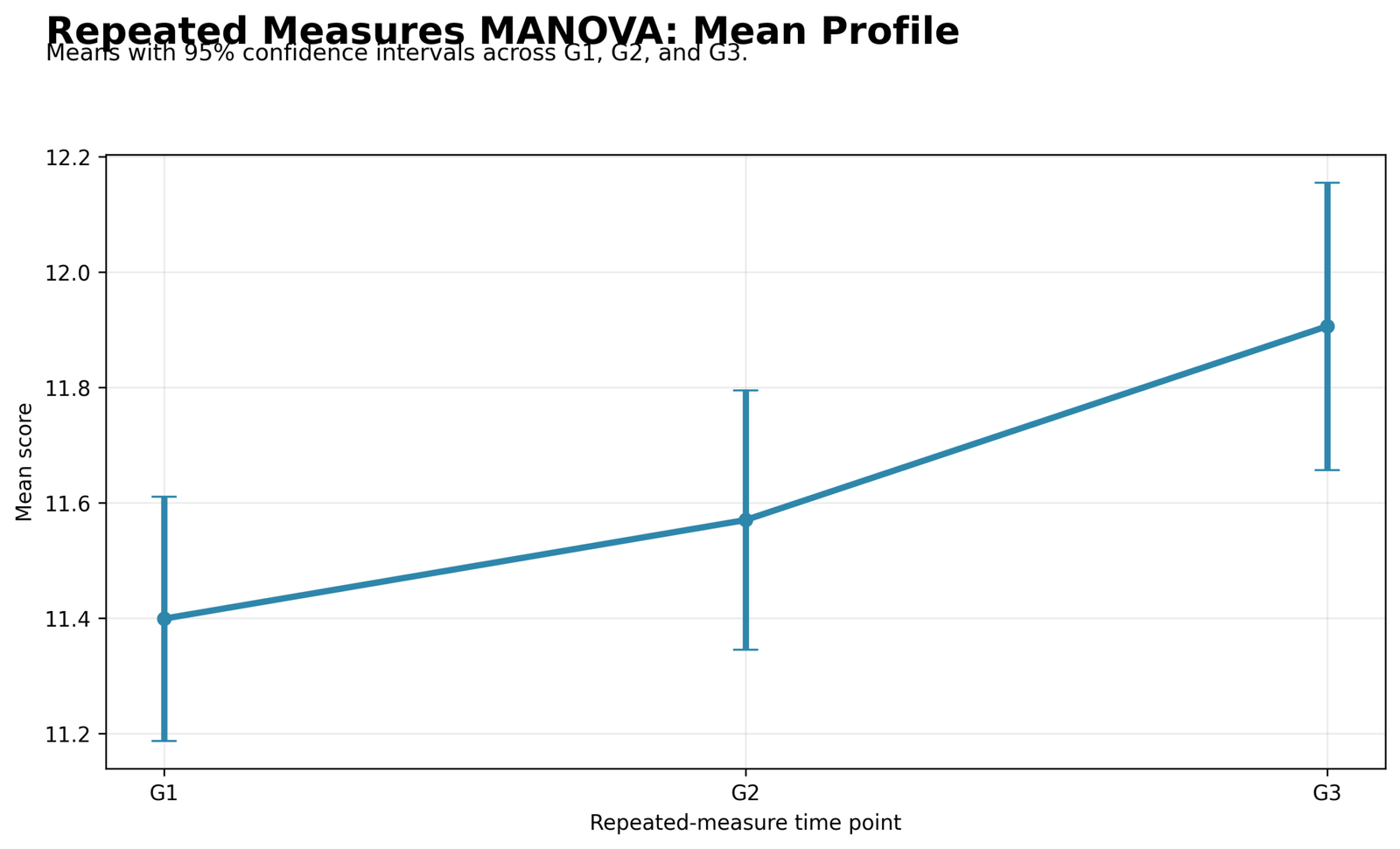
The mean profile chart shows that the repeated-measure average rises across the grade sequence. G1 is about 11.40, G2 is about 11.57, and G3 is about 11.91.
This chart gives the simplest visual explanation of the result. The profile is not flat. The average student score increases across the repeated measures, especially by the time G3 is reached.
Python Chart 2: Individual Repeated-Measure Trajectories
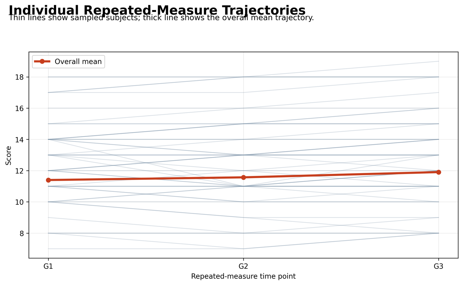
The individual trajectory plot shows that not every student follows the same path. Some individual lines rise, some are flat, and some fall between G1, G2 and G3.
The thick overall line still rises across the repeated outcomes. This means individual variation exists, but the average multivariate repeated-measure trend remains positive.
Python Chart 3: Change Score Boxplots
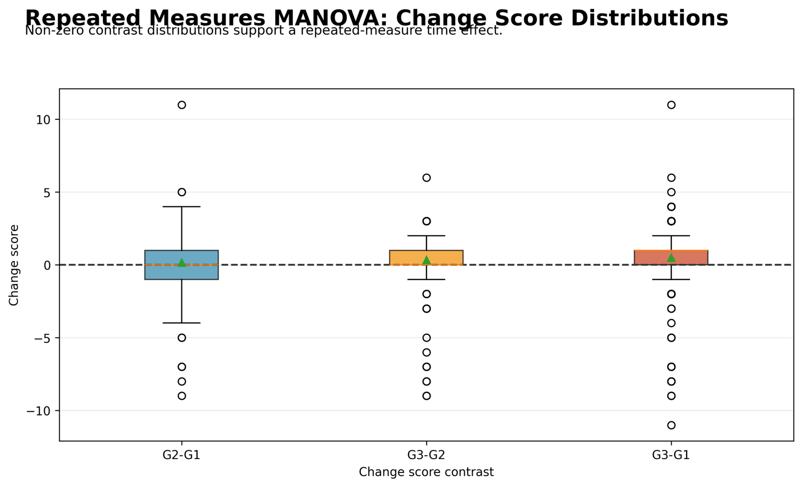
The change-score boxplots show that the distributions are centered around small positive changes. The G3 − G1 contrast has the clearest positive average, while G2 − G1 is smaller.
The chart also shows outlying positive and negative changes. This is important because repeated-measure change is not identical for every student. The MANOVA result tests the average change vector while still allowing individual differences around that vector.
Python Chart 4: Repeated-Measure Correlation Heatmap
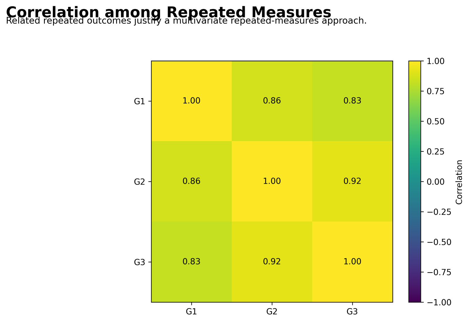
The correlation heatmap shows strong positive relationships among the repeated outcomes. G1 and G2 correlate .86, G1 and G3 correlate .83, and G2 and G3 correlate .92.
This chart supports the multivariate repeated-measures setup. The repeated outcomes are strongly connected, especially G2 and G3, but they are not identical. That makes a joint repeated-measure test meaningful.
Python Chart 5: Repeated-Measure Profiles by Studytime Group
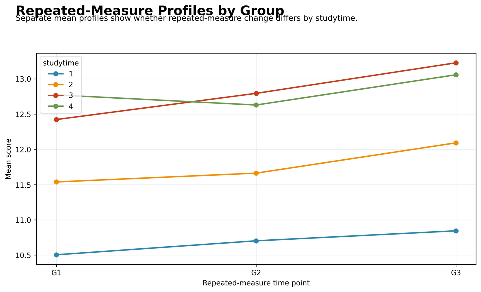
The group profile chart shows that studytime group 1 has the lowest grade profile, group 2 is higher, and groups 3 and 4 are in the highest range. Most groups show an upward movement toward G3.
The lines are not perfectly parallel, but the SPSS multivariate interaction test does not show a significant Time × studytime effect at alpha .05. The practical conclusion is that the grade profile rises overall, while studytime group differences mainly reflect different average grade levels.
Python Chart 6: Hotelling T² Summary for Time Effect
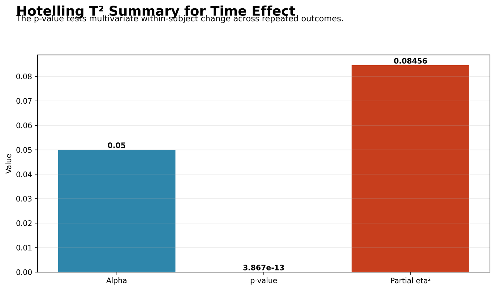
The Hotelling T² summary chart shows alpha = .05, p = 3.867e-13 and partial eta squared = 0.08456. The p-value is far below alpha.
This chart is the main Python decision output. It confirms that the repeated-measure change vector is statistically significant and that the time effect has a meaningful effect-size estimate.
Python Chart 7: Mean Change Scores with 95% Confidence Intervals
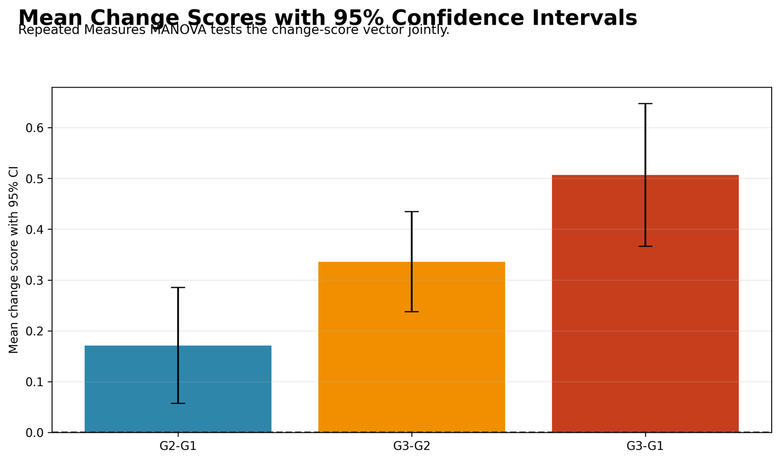
The mean change chart shows that G2 − G1 is about 0.17, G3 − G2 is about 0.34, and G3 − G1 is about 0.51. The largest mean change is the full G1 to G3 contrast.
The confidence intervals help explain the direction and uncertainty of each change. The overall pattern is positive, with the strongest practical change occurring between the first and final repeated measure.
Python Chart 8: Repeated Measures MANOVA Summary Table
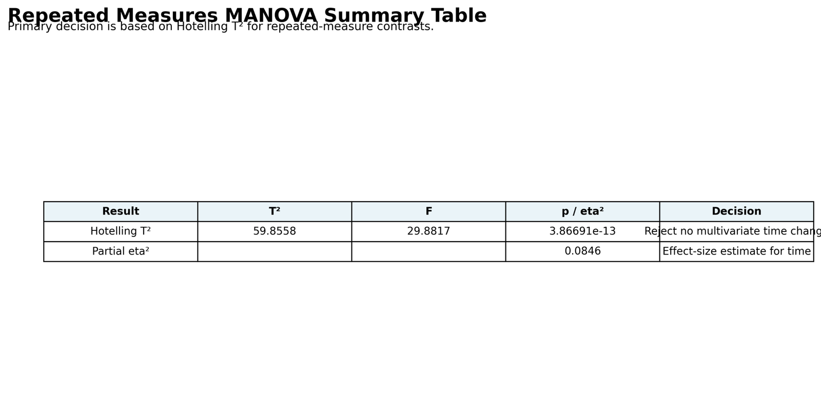
The summary table reports Hotelling T² = 59.8558, F = 29.8817, p = 3.86691e-13 and partial η² = 0.0846.
This table is the best compact Python result for reporting. It gives the statistic, inferential decision and effect-size estimate in one place.
R Chart-by-Chart Validation
The R validation charts repeat the same Repeated Measures MANOVA workflow in a second software environment. They confirm the mean profile, individual trajectories, change-score distributions, correlation heatmap, group profiles, Hotelling result, change-score confidence intervals and summary table.
R Chart 1: Repeated-Measure Mean Profile
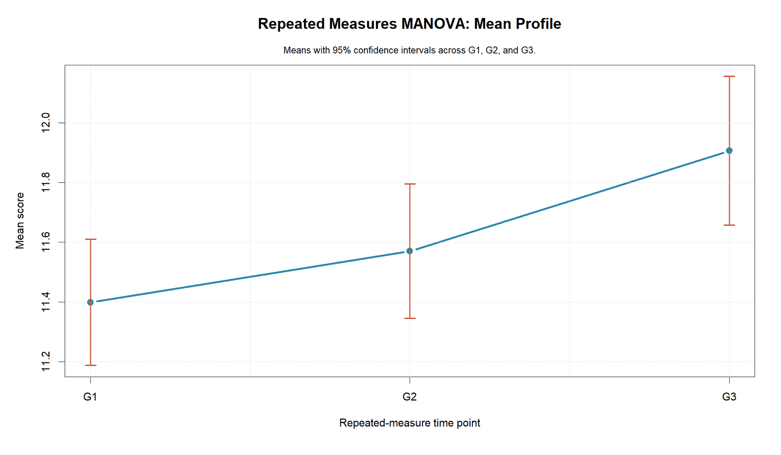
The R mean profile confirms the Python result. The average grade profile rises from G1 through G3.
This validation shows that the positive repeated-measure trend is stable across software workflows.
R Chart 2: Individual Repeated-Measure Trajectories
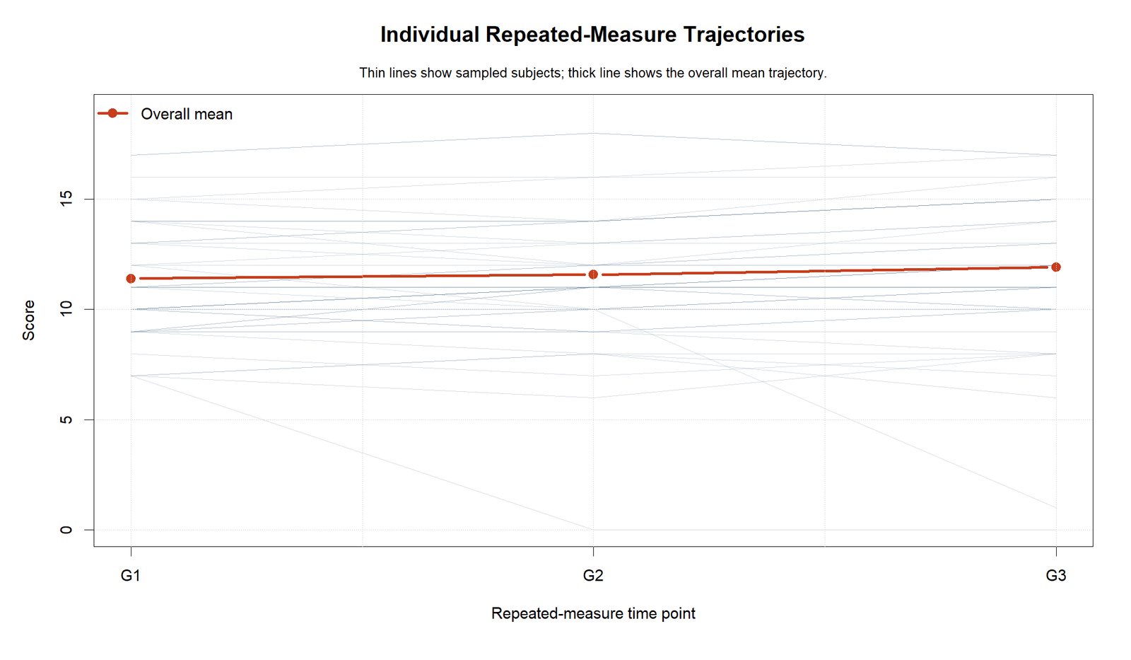
The R trajectory plot confirms that individual students vary in their repeated-score paths. Some trajectories move upward, while others move less consistently.
The average path remains upward, supporting the same multivariate time-change conclusion.
R Chart 3: Change Score Boxplots
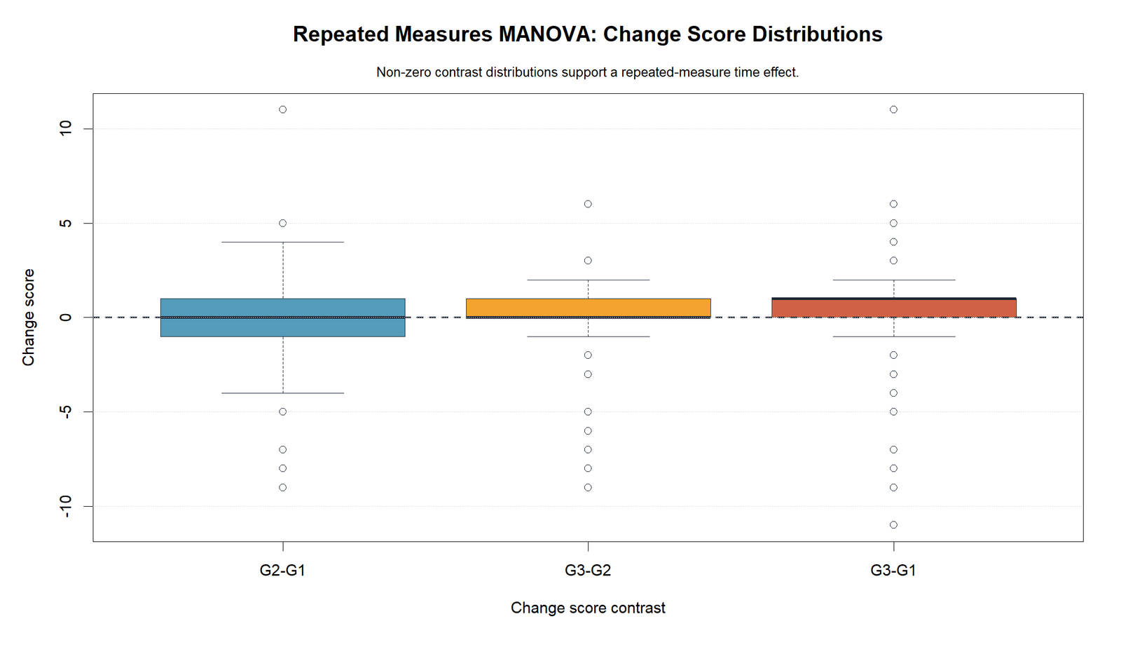
The R boxplots confirm the same change-score structure. The average changes are positive, but individual change scores vary around the mean.
This supports the repeated-measures MANOVA logic because the test evaluates a multivariate change vector rather than assuming identical change for every subject.
R Chart 4: Repeated-Measure Correlation Heatmap
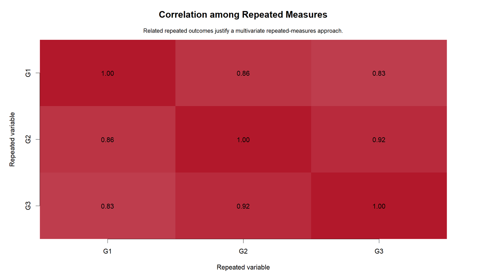
The R heatmap confirms strong repeated-measure correlations. G2 and G3 remain the most strongly related measures.
This validates the decision to treat the grade outcomes as a repeated multivariate profile.
R Chart 5: Repeated-Measure Profiles by Studytime Group
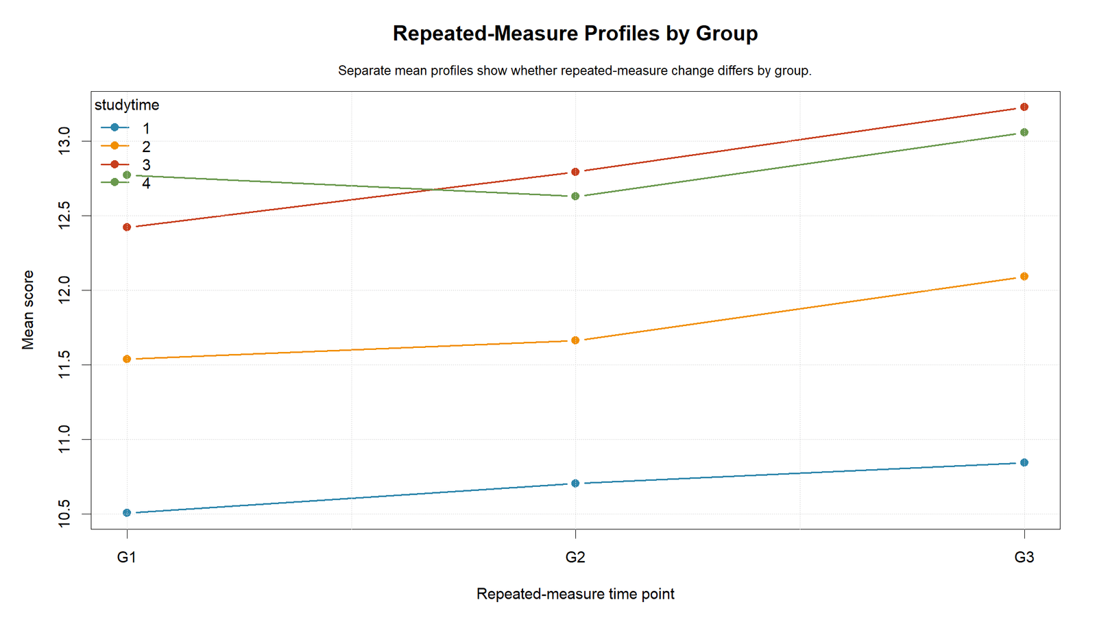
The R group profile chart confirms that studytime groups differ in grade level. Group 1 is lowest, group 2 is higher, and groups 3 and 4 are highest.
The practical pattern matches the Python chart. The repeated grade profile rises overall, while studytime group membership mainly separates students by average grade level.
R Chart 6: Hotelling T² Summary for Time Effect
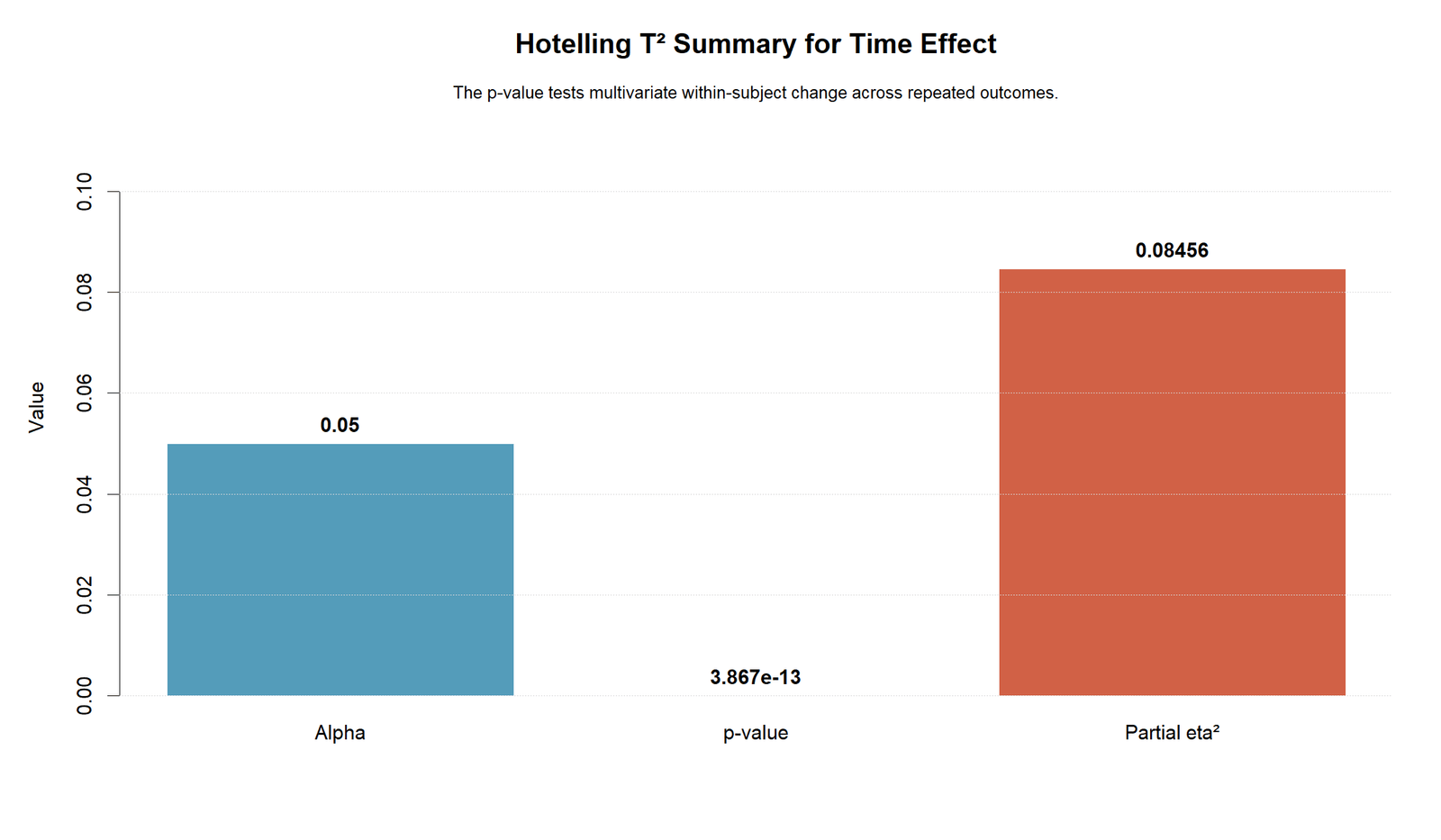
The R Hotelling summary confirms that the p-value is far below alpha and the partial eta squared value is meaningful.
This validates the main multivariate time-effect result outside Python.
R Chart 7: Mean Change Scores with 95% Confidence Intervals
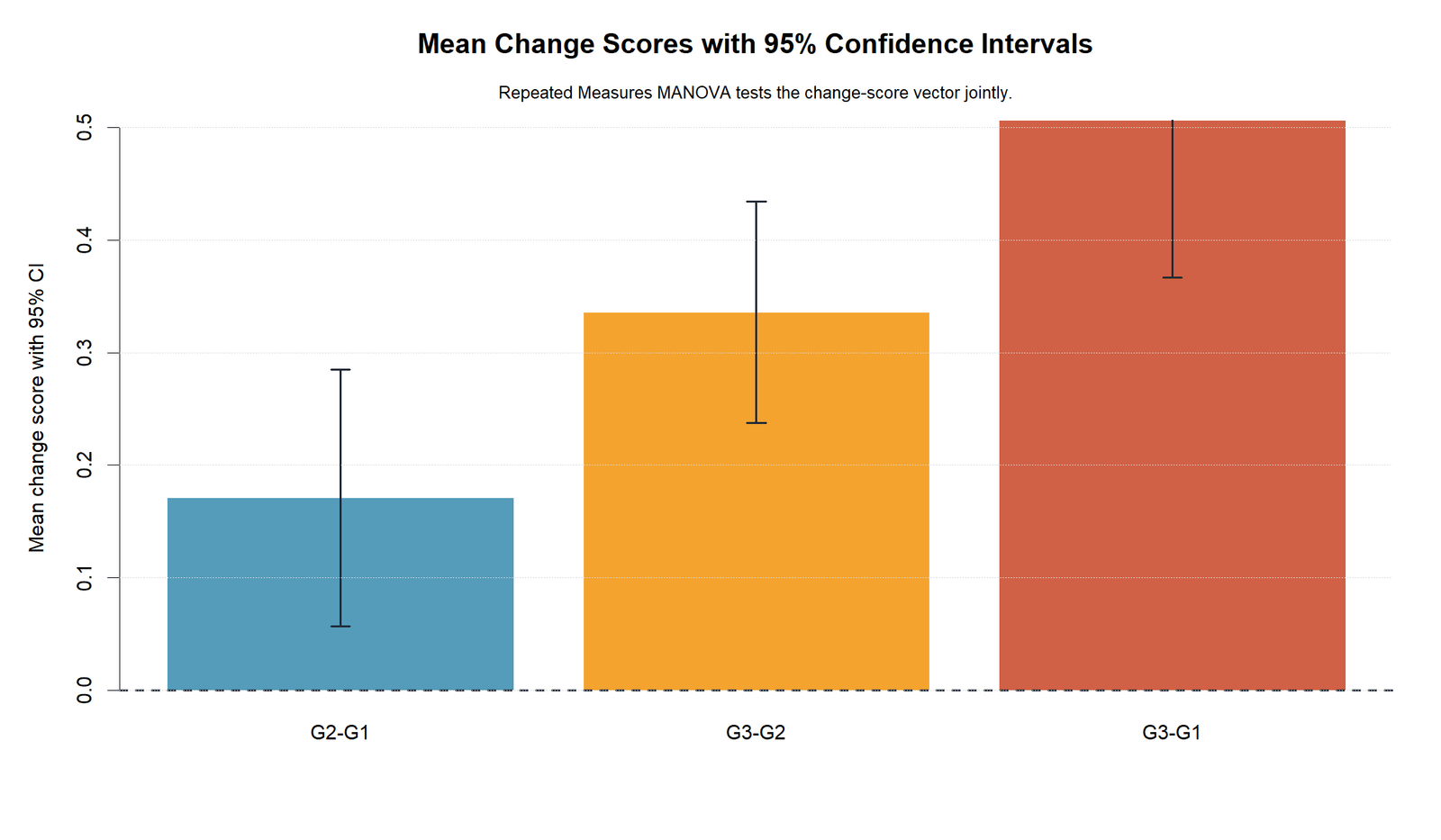
The R mean change chart confirms the same ordering: G3 − G1 is the largest change, G3 − G2 is next, and G2 − G1 is the smallest.
This supports the final interpretation that most of the average improvement is seen by the final repeated measurement.
R Chart 8: Repeated Measures MANOVA Summary Table
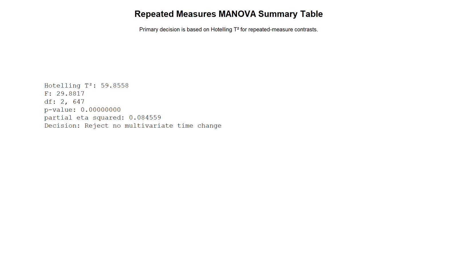
The R summary table confirms the same formal result as the Python table. The repeated-measure change vector is statistically significant.
This software validation strengthens the final report because Python, R and SPSS all support a significant repeated-measure time effect.
SPSS, R, Python and Excel Workflows for Repeated Measures MANOVA
The same Repeated Measures MANOVA workflow can be reproduced in SPSS, R, Python and Excel. Python and R can run the Hotelling T² change-vector test directly. SPSS can run the GLM repeated-measures multivariate tests. Excel can calculate means, change scores and correlation matrices, but SPSS, R or Python should be used for the formal MANOVA test.
SPSS Workflow
| Step | SPSS Menu or Syntax | Purpose |
|---|---|---|
| Open dataset | File > Open > Data | Load G1, G2, G3 and optional studytime. |
| Define repeated factor | Analyze > General Linear Model > Repeated Measures | Create Time with 3 levels. |
| Assign repeated variables | Time 1 = G1, Time 2 = G2, Time 3 = G3 | Connect columns to repeated levels. |
| Add between factor | studytime as between-subject factor | Test optional Time × studytime interaction. |
| Request output | Descriptives, effect size, homogeneity tests and profile plot | Support interpretation and assumptions. |
| Read multivariate table | Pillai, Wilks, Hotelling, Roy | Report repeated-measures MANOVA decision. |
| Export output | OUTPUT EXPORT | Save SPSS output PDF. |
R Workflow
| Step | R Action | Purpose |
|---|---|---|
| Read data | read.csv("dataset.csv") | Load G1, G2 and G3. |
| Create change scores | D1 = G2 - G1, D2 = G3 - G1 | Build repeated-measure contrast vector. |
| Compute mean vector | colMeans(D) | Estimate average repeated changes. |
| Compute covariance matrix | cov(D) | Estimate covariance among changes. |
| Run Hotelling T² | Manual matrix formula | Test whether the change vector differs from zero. |
| Validate with charts | Mean profile, change boxplots, heatmap and summary table | Explain the result visually. |
Python Workflow
| Step | Python Action | Purpose |
|---|---|---|
| Read data | pandas.read_csv() | Load repeated grade columns. |
| Clean complete cases | dropna(subset=["G1","G2","G3"]) | Use subjects with all repeated measures. |
| Create change matrix | np.column_stack([G2-G1, G3-G1]) | Build repeated-measure contrast matrix. |
| Calculate Hotelling T² | n * mean.T @ inv(cov) @ mean | Run multivariate time-effect test. |
| Convert to F | F conversion formula | Obtain p-value. |
| Create charts | Profiles, boxplots, heatmap and summary table | Explain and validate the result. |
Excel Workflow
| Excel Task | Formula or Tool | Purpose |
|---|---|---|
| Prepare wide data | Subject ID, G1, G2, G3 | Keep repeated measures on the same row. |
| Calculate means | =AVERAGE() | Get repeated-measure means. |
| Calculate change scores | =G2-G1, =G3-G1, =G3-G2 | Summarize within-subject change. |
| Create correlation matrix | =CORREL() | Check repeated-measure relationships. |
| Create charts | Line chart and boxplots | Visualize repeated profile and changes. |
| Formal MANOVA | Use SPSS, R or Python | Excel is not recommended for the full Hotelling T² MANOVA test. |
Code Blocks for Repeated Measures MANOVA
SPSS Syntax for Repeated Measures MANOVA
* Repeated Measures MANOVA in SPSS.
* Repeated measures: G1, G2, G3.
* Optional between-subject factor: studytime.

TITLE "Repeated Measures MANOVA: G1, G2 and G3".

GLM G1 G2 G3 BY studytime
  /WSFACTOR=Time 3 Polynomial
  /MEASURE=Grade
  /METHOD=SSTYPE(3)
  /PRINT=DESCRIPTIVE ETASQ HOMOGENEITY
  /PLOT=PROFILE(Time*studytime)
  /CRITERIA=ALPHA(.05)
  /WSDESIGN=Time
  /DESIGN=studytime.

OUTPUT EXPORT
  /CONTENTS EXPORT=VISIBLE
  /PDF DOCUMENTFILE="repeated_measures_manova_spss_output.pdf".
Python Code for Repeated Measures MANOVA
import pandas as pd
import numpy as np
from scipy import stats

df = pd.read_csv("dataset.csv")

for col in ["G1", "G2", "G3"]:
    df[col] = pd.to_numeric(df[col], errors="coerce")

wide = df[["G1", "G2", "G3"]].dropna().copy()

# Repeated-measure change-score matrix
# Two independent contrasts for three repeated outcomes
D = np.column_stack([
    wide["G2"] - wide["G1"],
    wide["G3"] - wide["G1"]
])

n, p = D.shape

mean_vector = D.mean(axis=0)
cov_matrix = np.cov(D, rowvar=False)

# Hotelling T-squared
T2 = n * mean_vector.T @ np.linalg.inv(cov_matrix) @ mean_vector

# Convert T2 to F
F_value = ((n - p) / (p * (n - 1))) * T2
df1 = p
df2 = n - p
p_value = stats.f.sf(F_value, df1, df2)

partial_eta_squared = T2 / (T2 + n - 1)

print("Mean vector:", mean_vector)
print("Hotelling T2:", T2)
print("F:", F_value)
print("df1:", df1)
print("df2:", df2)
print("p-value:", p_value)
print("Partial eta squared:", partial_eta_squared)

# Repeated-measure means
print(wide[["G1", "G2", "G3"]].mean())

# Change score means
wide["G2_G1"] = wide["G2"] - wide["G1"]
wide["G3_G2"] = wide["G3"] - wide["G2"]
wide["G3_G1"] = wide["G3"] - wide["G1"]
print(wide[["G2_G1", "G3_G2", "G3_G1"]].mean())

# Repeated-measure correlation matrix
print(wide[["G1", "G2", "G3"]].corr())
R Code for Repeated Measures MANOVA
# Repeated Measures MANOVA in R using Hotelling T-squared

library(tidyverse)

df <- read.csv("dataset.csv")

df$G1 <- as.numeric(df$G1)
df$G2 <- as.numeric(df$G2)
df$G3 <- as.numeric(df$G3)

wide <- df %>%
  select(G1, G2, G3) %>%
  drop_na()

D <- cbind(
  G2_G1 = wide$G2 - wide$G1,
  G3_G1 = wide$G3 - wide$G1
)

n <- nrow(D)
p <- ncol(D)

mean_vector <- colMeans(D)
cov_matrix <- cov(D)

T2 <- n * t(mean_vector) %*% solve(cov_matrix) %*% mean_vector
T2 <- as.numeric(T2)

F_value <- ((n - p) / (p * (n - 1))) * T2
df1 <- p
df2 <- n - p
p_value <- pf(F_value, df1, df2, lower.tail = FALSE)

partial_eta_squared <- T2 / (T2 + n - 1)

T2
F_value
df1
df2
p_value
partial_eta_squared

colMeans(wide[, c("G1", "G2", "G3")])
cor(wide[, c("G1", "G2", "G3")])
Excel Notes for Repeated Measures MANOVA
Excel support workflow:

1. Keep repeated measures on the same row:
   Subject_ID | G1 | G2 | G3

2. Calculate repeated-measure means:
   G1 mean = AVERAGE(G1_range)
   G2 mean = AVERAGE(G2_range)
   G3 mean = AVERAGE(G3_range)

3. Calculate change scores:
   G2_G1 = G2 - G1
   G3_G2 = G3 - G2
   G3_G1 = G3 - G1

4. Calculate mean changes:
   =AVERAGE(change_score_range)

5. Create correlation matrix:
   =CORREL(G1_range, G2_range)
   =CORREL(G1_range, G3_range)
   =CORREL(G2_range, G3_range)

6. Create charts:
   - repeated-measure mean profile
   - change-score boxplots
   - correlation matrix
   - group profiles if a between-subject factor exists

7. Formal MANOVA:
   Use SPSS, Python or R for Hotelling T², Wilks, Pillai, Hotelling Trace or Roy's Root.
APA Reporting Wording
When reporting Repeated Measures MANOVA, include the repeated outcomes, the multivariate test statistic, F statistic, degrees of freedom, p-value, effect size, mean profile and change-score direction. When using SPSS, also state whether the Time × between-subject factor interaction was significant.
APA-style report: A repeated measures MANOVA was conducted to test whether student grade outcomes changed across G1, G2 and G3. The Hotelling T² test of the repeated-measure change vector was significant, T² = 59.8558, F = 29.8817, p = 3.86691e-13, partial η² = 0.0846. Mean scores increased from G1 (M ≈ 11.40) to G2 (M ≈ 11.57) and G3 (M ≈ 11.91). The largest mean change was from G1 to G3, approximately 0.51 points. SPSS multivariate GLM output also showed a significant Time effect, F(2, 644) = 16.435, p < .001, partial η² = .049, while the Time × studytime interaction was not significant by Pillai’s Trace, p = .089.
Short reporting version: The repeated-measure grade profile changed significantly across G1, G2 and G3. Hotelling T² = 59.8558, F = 29.8817, p < .001, partial η² = 0.0846. Mean scores increased from 11.40 to 11.57 to 11.91.
Common Mistakes
| Mistake | Why It Is Wrong | Correct Practice |
|---|---|---|
| Using independent one-way ANOVA for repeated outcomes | G1, G2 and G3 are measured on the same students. | Use repeated-measures ANOVA or repeated-measures MANOVA. |
| Ignoring repeated-measure correlations | The repeated outcomes are strongly correlated. | Report the correlation matrix and use within-subject logic. |
| Confusing RM ANOVA and RM MANOVA | RM ANOVA uses a univariate within-subject test; RM MANOVA uses a multivariate repeated-change test. | Name the method clearly and report the correct statistic. |
| Reporting only the p-value | The p-value does not explain practical direction. | Report means, change scores and partial eta squared. |
| Ignoring sphericity in the univariate layer | Mauchly’s test is significant in the SPSS output. | Use Greenhouse-Geisser Correction or Huynh-Feldt Correction for univariate RM ANOVA reporting. |
| Overstating the Time × studytime interaction | The SPSS multivariate interaction is not significant by Pillai p = .089. | Describe studytime as separating average grade level, not as a clearly significant repeated-change interaction. |
When to Use Repeated Measures MANOVA
Use Repeated Measures MANOVA when the same subjects have multiple related repeated outcomes and the research question focuses on whether the repeated outcome profile changes jointly. It is especially useful when a multivariate approach to repeated contrasts is preferred or when the analyst wants to avoid relying only on the sphericity-based univariate repeated-measures ANOVA layer.
| Situation | Use Repeated Measures MANOVA? | Reporting Note |
|---|---|---|
| Same subjects measured at G1, G2 and G3 | Yes | Use a within-subject multivariate time-effect test. |
| Only one repeated outcome pair | Usually no | Use a paired t test. |
| Three or more independent groups | No | Use One Way ANOVA or One Way MANOVA. |
| Repeated factor plus between-subject factor | Yes, with interaction interpretation | Compare with Mixed MANOVA. |
| Sphericity is violated in univariate RM ANOVA | MANOVA approach may help | Still report assumptions and the exact method used. |
Repeated Measures MANOVA should be compared with Mixed MANOVA, Mixed ANOVA, One Way MANOVA, One Way ANOVA, One Way ANCOVA, Fixed Effects ANOVA, Factorial ANOVA, ANOVA Assumptions, and ANOVA Effect Size.
Downloads and Resources for Repeated Measures MANOVA
Use these resources to reproduce the Repeated Measures MANOVA workflow. The Python report, R report and SPSS output PDF are included as verification files. Script and workbook placeholders can be replaced after the final downloadable files are uploaded to the WordPress Media Library.
Download Dataset
Practice dataset with G1, G2 and G3 repeated measures.
Download Repeated Measures MANOVA Python Report PDF
Python report PDF for Hotelling T², change scores, correlations and charts.
Download Repeated Measures MANOVA R Report PDF
R validation PDF for repeated-measure MANOVA interpretation.
Download Repeated Measures MANOVA SPSS Output PDF
SPSS output PDF for multivariate Time effect, Time × studytime interaction and assumptions.
Download Python Script
Python code for repeated-measures MANOVA, Hotelling T² and charts.
Download R Script and Excel Workbook
R workflow and Excel support workbook for repeated-measures MANOVA summaries.
FAQs About Repeated Measures MANOVA
What is Repeated Measures MANOVA?
Repeated Measures MANOVA is a multivariate within-subject analysis used to test whether related repeated outcomes measured on the same subjects change jointly.
What repeated measures were used in this example?
The repeated measures were G1, G2 and G3 grade scores for the same students.
What was the Python Hotelling T² result?
The Python Hotelling T² result was T² = 59.8558, F = 29.8817, p = 3.86691e-13 and partial η² = 0.0846.
Was the repeated-measure time effect significant?
Yes. Both the Python Hotelling T² result and the SPSS multivariate Time effect showed a significant repeated-measure change.
What were the repeated-measure means?
The means were approximately 11.40 for G1, 11.57 for G2 and 11.91 for G3.
Which mean change was largest?
The largest mean change was G3 − G1, about 0.51 points.
Were the repeated measures correlated?
Yes. G1–G2 correlated .86, G1–G3 correlated .83 and G2–G3 correlated .92.
Was the Time × studytime interaction significant in SPSS?
No. The SPSS multivariate Time × studytime interaction was not significant by Pillai’s Trace, p = .089.
Can Repeated Measures MANOVA be done in Excel?
Excel can calculate means, change scores and correlations, but SPSS, R or Python should be used for the formal Repeated Measures MANOVA test.
How do I report this Repeated Measures MANOVA in APA style?
A concise report is: The repeated-measure grade profile changed significantly across G1, G2 and G3, Hotelling T² = 59.8558, F = 29.8817, p < .001, partial η² = 0.0846.

