Repeated Measures ANOVA, Sphericity, Epsilon Correction and Corrected P-Values
Huynh Feldt Correction: Formula, Interpretation, SPSS, Python, R and Excel Guide
Huynh Feldt Correction is a repeated measures ANOVA correction used when the sphericity assumption is not fully satisfied. It adjusts the degrees of freedom through an epsilon value so that the within-subjects F test is interpreted more safely. This Salar Cafe guide explains Huynh Feldt Correction with SPSS output, Python charts, R validation charts, epsilon comparison, corrected p-values, difference score variances, covariance heatmap, individual profiles, group mean profiles, Excel workflow, APA reporting, and common interpretation mistakes.
Google AdSense top placement reserved here
Quick Answer: Huynh Feldt Correction Result
The Huynh Feldt Correction is used in repeated measures ANOVA when the equal-variance pattern among repeated-measure difference scores is questionable. In ordinary repeated measures ANOVA, the uncorrected within-subjects test assumes sphericity. When this assumption is violated, the uncorrected p-value can become too optimistic. The Huynh-Feldt correction adjusts the degrees of freedom and produces a corrected p-value that is more appropriate for the actual repeated-measures covariance pattern.
In practical reporting, the decision begins with Mauchly’s Test of Sphericity. If Mauchly’s test is significant, the sphericity assumption is violated, and a correction such as Greenhouse-Geisser Correction or Huynh-Feldt Correction should be interpreted. Huynh-Feldt is usually less conservative than Greenhouse-Geisser because its epsilon is often larger. This means it corrects the degrees of freedom but does not reduce them as severely.
Hypothesis-style interpretation: The null hypothesis for the repeated measures ANOVA says that the population means are equal across the repeated conditions. The alternative hypothesis says that at least one repeated-measure mean differs. If the Huynh-Feldt corrected p-value is below the chosen alpha level, usually .05, the null hypothesis is rejected after adjusting for sphericity violation. If the corrected p-value is not below .05, the researcher fails to reject the null hypothesis after correction.
Final interpretation: Huynh Feldt Correction should be reported when repeated measures ANOVA requires an adjusted sphericity result and the Huynh-Feldt row is suitable for interpretation. The correction does not change the repeated-measures means. It changes the degrees of freedom used to evaluate the F statistic, which can change the p-value and therefore the hypothesis decision.
Important note: Do not report the uncorrected repeated measures ANOVA result as the final result when sphericity is violated. If Mauchly’s test is significant, interpret a corrected row such as Greenhouse-Geisser or Huynh-Feldt. The selected row should be reported with adjusted degrees of freedom, F value, p-value, and effect size where available.
Table of Contents
- What Is Huynh Feldt Correction?
- Huynh Feldt Correction Formula
- Null and Alternative Hypotheses
- Dataset and Variables Used
- Verified SPSS Output Interpretation
- Python Chart-by-Chart Interpretation
- R Chart-by-Chart Validation
- SPSS, R, Python and Excel Workflows
- Code Blocks for Huynh Feldt Correction
- APA Reporting Wording
- Common Mistakes
- When to Use Huynh Feldt Correction
- Downloads and Resources
- Related Guides
- FAQs
What Is Huynh Feldt Correction?
Huynh Feldt Correction is a statistical adjustment used in repeated measures ANOVA when the sphericity assumption is violated or questionable. Repeated measures ANOVA is used when the same subjects are measured across multiple time points, test occasions, treatment stages, or experimental conditions. Because the same subjects appear repeatedly, the measurements are correlated. That repeated-measures structure creates a special assumption called sphericity.
Sphericity means that the variances of the pairwise differences between repeated conditions are approximately equal. For example, if a student performance score is measured at Time 1, Time 2, Time 3 and Time 4, the variance of Time 1 minus Time 2 should be comparable to the variance of Time 1 minus Time 3, Time 1 minus Time 4, Time 2 minus Time 3 and so on. When these difference-score variances are very unequal, sphericity is violated.
The Huynh-Feldt correction solves the problem by multiplying the original degrees of freedom by an epsilon estimate. This produces adjusted degrees of freedom and a corrected p-value. In many outputs, especially SPSS repeated measures ANOVA, Huynh-Feldt appears beside other rows such as Sphericity Assumed, Greenhouse-Geisser and Lower-bound. For a complete assumption workflow, compare this guide with Mauchly’s Test of Sphericity, Greenhouse-Geisser Correction, Q-Q Plot Normality Check, and P-P Plot Normality Check.
Practical meaning: Huynh Feldt Correction does not change the sample means, line chart pattern, or repeated-measure profile. It changes the inferential test by correcting the degrees of freedom. Therefore, the graph may show the same trend, but the final p-value must be read from the corrected row when sphericity is not satisfied.
Huynh Feldt Correction Formula
The central idea behind Huynh Feldt Correction is the epsilon adjustment. Epsilon represents how much the repeated-measures degrees of freedom should be reduced to account for sphericity violation.
Here, εHF is the Huynh-Feldt epsilon. If epsilon is close to 1, the sphericity problem is mild. If epsilon is much lower, the correction becomes stronger. The Huynh-Feldt epsilon is commonly larger than the Greenhouse-Geisser epsilon, so Huynh-Feldt is usually less conservative.
The repeated measures F ratio itself follows the usual ANOVA logic:
The correction does not usually change the conceptual F ratio. Instead, it changes how the F statistic is evaluated by adjusting the numerator and denominator degrees of freedom. This is why the same F value may appear with different significance values across the Sphericity Assumed, Greenhouse-Geisser, Huynh-Feldt and Lower-bound rows.
| Correction Row | Meaning | Typical Interpretation |
|---|---|---|
| Sphericity Assumed | No correction is applied. | Use this row only when sphericity is satisfied. |
| Greenhouse-Geisser | A conservative epsilon correction is applied. | Often used when sphericity violation is stronger or epsilon is low. |
| Huynh-Feldt | A less conservative epsilon correction is applied. | Often used when epsilon is higher and the correction is not extremely severe. |
| Lower-bound | The strongest correction is applied. | Usually treated as a very conservative reference row. |
Formula caution: Huynh-Feldt Correction is not selected by looking only at whether the final p-value is convenient. The correction should be selected based on sphericity diagnostics, epsilon values, study design, and accepted reporting practice.
Null and Alternative Hypotheses
Huynh Feldt Correction is part of the repeated measures ANOVA decision process. The correction itself is not the research hypothesis; it is the adjusted way of testing the repeated-measures effect when sphericity is not fully met.
| Hypothesis Type | Null Hypothesis | Alternative Hypothesis | Decision Rule |
|---|---|---|---|
| Repeated measures main effect | Mean scores are equal across all repeated conditions or time points. | At least one repeated-condition mean is different. | Reject H0 if the corrected p-value is below alpha. |
| Sphericity assumption | The variances of pairwise difference scores are equal enough for sphericity. | The pairwise difference-score variances are not equal enough. | If Mauchly’s test p < .05, use a corrected ANOVA row. |
| Huynh-Feldt corrected decision | After correction, there is no statistically significant repeated-measures effect. | After correction, there is a statistically significant repeated-measures effect. | Use the Huynh-Feldt corrected p-value for the decision. |
Hypothesis-style decision: If the Huynh-Feldt corrected p-value is significant, reject the null hypothesis and conclude that the repeated-measures means differ after correcting for sphericity. If the corrected p-value is not significant, fail to reject the null hypothesis and report that the repeated-measures effect was not statistically significant after correction.
Interpretation nuance: A significant corrected result tells you that not all repeated-measure means are equal. It does not automatically tell you which time points or conditions differ. For that, use planned contrasts, pairwise comparisons, confidence intervals, and effect size interpretation. See confidence interval and effect size guides for reporting support.
Dataset and Variables Used
This Huynh Feldt Correction guide is written for a repeated measures dataset where the same cases are measured more than twice. The repeated factor may be time, test occasion, treatment phase, learning stage, experimental condition, or any within-subject factor. The dependent variable must be a quantitative outcome measured repeatedly for the same subjects.
| Dataset Component | Description | Why It Matters for Huynh-Feldt |
|---|---|---|
| Subject ID | A unique identifier for each participant, student, patient, respondent, or case. | Repeated measures ANOVA needs to know which observations belong to the same subject. |
| Within-subject factor | The repeated condition, such as Time 1, Time 2, Time 3 and Time 4. | Sphericity is only relevant when the within-subject factor has at least three levels. |
| Dependent variable | The numeric outcome measured repeatedly. | The repeated measures ANOVA tests whether the outcome mean changes across levels. |
| Difference scores | Pairwise differences between repeated conditions. | The equality of their variances is the practical meaning of sphericity. |
| Grouping variable | An optional between-subject factor such as group, school, gender, treatment, or class. | Group mean profiles can show whether repeated patterns differ across categories. |
Before running repeated measures ANOVA, review the data using descriptive statistics, frequency distribution, histogram interpretation, box plot interpretation, and five-number summary. These checks help identify strange values, unusual spread, distribution shape, and practical data issues before interpreting the corrected ANOVA result.
Google AdSense middle placement reserved here
Verified SPSS Output Interpretation
The SPSS output for this Huynh Feldt Correction guide is available here: Huynh Feldt Correction SPSS Output PDF.
In SPSS, Huynh-Feldt Correction appears in the repeated measures ANOVA output under the Tests of Within-Subjects Effects table. The main interpretation depends on three linked parts of the output: descriptive means, Mauchly’s test, and corrected within-subjects tests. The descriptive profile explains the direction of change. Mauchly’s test explains whether sphericity can be assumed. The Huynh-Feldt row provides the corrected inference when sphericity is violated or questionable.
SPSS Interpretation Table
| SPSS Output Item | What to Read | How to Interpret It | Reporting Use |
|---|---|---|---|
| Descriptive Statistics | Means and standard deviations for each repeated condition. | Shows whether the outcome increases, decreases, or changes non-linearly across time or conditions. | Use this to describe the practical pattern before reporting the F test. |
| Multivariate Tests | Pillai’s Trace, Wilks’ Lambda, Hotelling’s Trace and Roy’s Largest Root. | Provides an alternative repeated-measures perspective that does not require the same sphericity assumption as the univariate test. | Useful as supporting output, but the main guide here focuses on Huynh-Feldt corrected univariate results. |
| Mauchly’s Test of Sphericity | Chi-square, degrees of freedom and significance value. | If p < .05, sphericity is violated and corrected rows should be interpreted. | Report this before giving the corrected ANOVA result. |
| Epsilon Values | Greenhouse-Geisser, Huynh-Feldt and Lower-bound epsilon estimates. | Higher epsilon means less severe correction. Huynh-Feldt is usually less conservative than Greenhouse-Geisser. | Use epsilon to justify why the corrected degrees of freedom differ from the original df. |
| Tests of Within-Subjects Effects | The Huynh-Feldt row for the repeated factor. | Read adjusted df, F value and corrected significance from the Huynh-Feldt row. | This row is the core result when reporting Huynh Feldt Correction. |
| Estimated Marginal Means / Profile Plot | Mean pattern across repeated conditions. | Shows the direction and size of the repeated-measures pattern visually. | Use with charts for a reader-friendly explanation. |
SPSS Decision Summary
SPSS interpretation summary: If Mauchly’s test in the SPSS output is significant, the sphericity assumption should not be trusted. The repeated measures result should then be reported from a corrected row. The Huynh-Feldt row gives the corrected degrees of freedom and corrected p-value. If the Huynh-Feldt corrected p-value is significant, the repeated-measures effect remains significant after correction. If it is not significant, the apparent repeated-measures effect is not statistically supported after adjusting for sphericity.
Correct reporting logic: Describe the repeated-measures mean pattern first, mention whether Mauchly’s test indicated a sphericity problem, state that the Huynh-Feldt correction was applied, and then report the corrected F statistic with adjusted degrees of freedom, p-value and effect size. Do not report only the uncorrected row when the sphericity assumption is violated.
Important limitation: The SPSS PDF should be used to copy the exact numeric values for the final published statistical sentence. The interpretation framework in this post explains how to read and report the result without inventing unverified statistics.
Python Chart-by-Chart Interpretation
The Python charts show the Huynh Feldt Correction workflow visually. They explain the repeated means, epsilon comparison, corrected p-values, difference score variances, covariance structure, individual trajectories and group-level profiles. Each chart below includes descriptive alt text, image title, lazy loading, caption, detailed interpretation, and a decision/reporting conclusion.
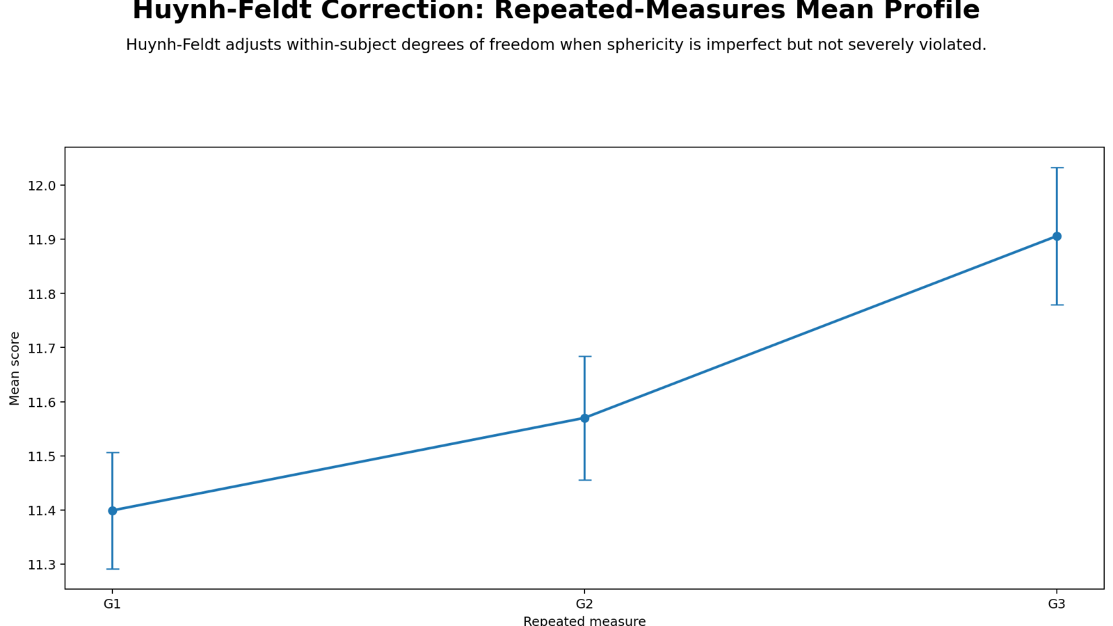
Python Chart 1: Repeated Measures Mean Profile

Detailed interpretation: This repeated measures mean profile is the first visual check in a Huynh Feldt Correction analysis. It shows whether the average outcome changes across the repeated conditions. A flat profile suggests little average change, while an upward, downward or curved profile suggests that the repeated factor may have a meaningful effect. This plot does not test sphericity directly, but it helps readers understand the practical direction of the repeated-measures pattern before the corrected ANOVA result is reported.
Decision/reporting conclusion: Use this chart to describe the repeated-measures trend in plain language. The final inferential decision should still come from the Huynh-Feldt corrected p-value if sphericity is violated.
Python Chart 2: Epsilon Comparison

Detailed interpretation: This epsilon comparison chart is central to the Huynh Feldt Correction topic. Epsilon values summarize how much the original repeated-measures degrees of freedom should be reduced. A value closer to 1 means the adjustment is mild, while a smaller value means stronger correction. Huynh-Feldt epsilon is usually larger than Greenhouse-Geisser epsilon, so it is often less conservative. The chart helps explain why corrected p-values can differ across correction methods.
Decision/reporting conclusion: Use this chart to justify the correction row selected for interpretation. If the Huynh-Feldt epsilon is reasonably high, the Huynh-Feldt corrected result may be appropriate to report, especially when supported by standard software output and accepted reporting practice.
Python Chart 3: Corrected P-Values

Detailed interpretation: This chart shows the practical consequence of correction. The uncorrected p-value is often the smallest because it assumes sphericity. Greenhouse-Geisser and Huynh-Feldt p-values are corrected for the sphericity issue. Huynh-Feldt is usually less conservative than Greenhouse-Geisser, so its corrected p-value may be closer to the uncorrected result. This chart helps prevent a common mistake: choosing the row with the most favorable p-value rather than the row justified by the assumption check.
Decision/reporting conclusion: If sphericity is violated, the corrected p-value should guide the hypothesis decision. Report whether the repeated-measures effect remains significant after Huynh-Feldt correction.
Python Chart 4: Difference Score Variances

Detailed interpretation: Sphericity is about the equality of variances of pairwise differences among repeated conditions. This chart directly visualizes those difference-score variances. If the bars are similar, the sphericity assumption is more plausible. If the bars differ strongly, the assumption is questionable and a correction becomes important. This chart is especially helpful for explaining sphericity to students because it turns an abstract assumption into a visible comparison.
Decision/reporting conclusion: Use this figure as visual support for the need to inspect Mauchly’s test and corrected ANOVA rows. Unequal difference-score variances strengthen the rationale for using Huynh-Feldt or Greenhouse-Geisser correction.
Python Chart 5: Covariance Matrix Heatmap

Detailed interpretation: The covariance matrix heatmap shows how repeated conditions are related to each other. Repeated measures data usually contain correlated observations because the same subjects are measured multiple times. A balanced covariance structure supports simpler repeated-measures assumptions, while uneven covariance patterns may indicate that the within-subject dependence structure is more complex. Although covariance heatmaps do not replace Mauchly’s test, they provide useful visual context.
Decision/reporting conclusion: Use this chart to explain the dependence structure behind the repeated measures ANOVA. The formal correction decision should still be based on sphericity diagnostics and corrected output rows.
Python Chart 6: Individual Profiles Spaghetti Plot

Detailed interpretation: The spaghetti plot shows how individual subjects change across repeated conditions. This is important because a mean profile can hide individual variation. If most lines move in the same direction, the mean trend is broadly shared. If lines cross heavily or vary widely, the average trend may not describe every subject well. This figure helps readers understand whether the repeated-measures effect is consistent or heterogeneous.
Decision/reporting conclusion: Use this chart as transparent support for the repeated measures pattern. It does not replace the Huynh-Feldt corrected ANOVA, but it improves interpretation by showing the subject-level data behind the mean profile.
Python Chart 7: Group Mean Profiles

Detailed interpretation: The group mean profile chart is useful when the dataset includes a between-subject grouping variable. Parallel lines suggest that groups change similarly across repeated conditions. Diverging or crossing lines suggest possible interaction patterns. Even when the main focus is Huynh Feldt Correction for the within-subject factor, group profiles help explain whether the repeated pattern is similar across subgroups.
Decision/reporting conclusion: Use this chart to describe group-level repeated trajectories. If a formal interaction test is part of the model, interpret the chart together with the corrected ANOVA output and relevant pairwise comparisons.
R Chart-by-Chart Validation
The R charts validate the Huynh Feldt Correction interpretation using a separate statistical environment. This is useful because repeated measures ANOVA and sphericity correction can be checked in more than one software tool. The R charts below mirror the Python workflow and provide visual confirmation of the repeated mean profile, epsilon comparison, corrected p-values, difference score variances, covariance heatmap, individual trajectories and group mean profiles.
R Chart 1: Repeated Measures Mean Profile

Detailed interpretation: The R repeated measures mean profile confirms the visual trend shown in the Python chart. When two software workflows show the same average pattern, confidence in the descriptive interpretation increases. The chart helps readers see whether the repeated factor is associated with increasing, decreasing or changing means.
Decision/reporting conclusion: Use this R chart as validation of the repeated-measures trend. The final statistical decision should still be reported from the corrected repeated measures ANOVA output.
R Chart 2: Epsilon Comparison

Detailed interpretation: The R epsilon comparison chart confirms the relative position of Huynh-Feldt compared with Greenhouse-Geisser and lower-bound correction. If Huynh-Feldt epsilon is larger, the adjusted degrees of freedom are reduced less strongly. This is why the Huynh-Feldt corrected p-value often differs from the more conservative Greenhouse-Geisser p-value.
Decision/reporting conclusion: Use this R validation chart to support the correction explanation. It helps readers understand why epsilon is central to corrected repeated measures inference.
R Chart 3: Corrected P-Values

Detailed interpretation: This R chart validates the corrected p-value pattern. If the p-values differ across correction methods, the chart makes the assumption impact visible. A result that looks significant in the uncorrected row may become weaker after correction. Conversely, a strong repeated-measures effect may remain significant even after Huynh-Feldt or Greenhouse-Geisser correction.
Decision/reporting conclusion: Use this chart to explain why corrected p-values matter. When sphericity is violated, report the corrected p-value rather than relying on the uncorrected significance value.
R Chart 4: Difference Score Variances

Detailed interpretation: This chart confirms whether pairwise difference-score variances are similar or uneven. The more uneven the bars, the more difficult it is to defend the uncorrected sphericity-assumed result. This R validation is useful because it reinforces the same assumption logic shown in the Python chart.
Decision/reporting conclusion: Use this chart to justify why the corrected ANOVA row should be examined. It is a strong teaching chart for explaining the basis of Huynh Feldt Correction.
R Chart 5: Covariance Matrix Heatmap

Detailed interpretation: The R covariance matrix heatmap gives another view of the dependence among repeated conditions. Similar covariance patterns suggest more regular within-subject structure, while irregular patterns may point to greater assumption complexity. This chart is not the final sphericity test, but it helps readers understand why repeated measures require special handling.
Decision/reporting conclusion: Use this heatmap as supporting evidence for the repeated-measures structure. Interpret it alongside Mauchly’s test, epsilon estimates and corrected p-values.
R Chart 6: Individual Profiles Spaghetti Plot

Detailed interpretation: The R spaghetti plot validates the individual-level pattern shown in Python. It shows whether most subjects follow the same repeated-measures direction or whether there is substantial variation across individuals. This is valuable because repeated measures ANOVA summarizes a pattern that may differ from subject to subject.
Decision/reporting conclusion: Use this chart to show transparency in the analysis. It supports the corrected ANOVA by showing the data structure behind the average repeated-measures effect.
R Chart 7: Group Mean Profiles

Detailed interpretation: The R group mean profile chart confirms whether subgroup patterns are parallel, divergent or crossing. When group lines are not parallel, the researcher may need to examine a group-by-time interaction. This chart is especially useful in educational, clinical and experimental designs where repeated changes may differ across groups.
Decision/reporting conclusion: Use this chart to support group-level interpretation. If interaction testing is included in the model, report it with corrected repeated-measures output and appropriate follow-up comparisons.
Google AdSense in-content placement reserved here
SPSS, R, Python and Excel Workflows for Huynh Feldt Correction
The Huynh Feldt Correction workflow is similar across software. The researcher first arranges repeated measures data correctly, runs repeated measures ANOVA, checks sphericity, reviews epsilon values, and reports the corrected result when needed.
SPSS Workflow
| Step | SPSS Menu or Syntax | Purpose |
|---|---|---|
| Open dataset | File > Open > Data | Load the repeated measures dataset. |
| Define repeated factor | Analyze > General Linear Model > Repeated Measures | Create the within-subject factor and specify the number of levels. |
| Assign variables | Move repeated variables into the within-subjects boxes. | Ensure the time points or conditions are in correct order. |
| Request output | Options, Plots and EM Means | Request descriptive statistics, effect sizes, profile plots and comparisons. |
| Check Mauchly’s test | Read Mauchly’s Test of Sphericity table. | Decide whether a correction is required. |
| Report correction | Read Tests of Within-Subjects Effects. | Report the Huynh-Feldt row if it is the appropriate corrected result. |
| Export output | File > Export or OUTPUT EXPORT | Save SPSS output as PDF for documentation. |
R Workflow
| Step | R Action | Purpose |
|---|---|---|
| Read data | read.csv() or readxl::read_excel() | Load the dataset into R. |
| Reshape data | pivot_longer() | Convert wide repeated-measures columns into long format if needed. |
| Run repeated measures ANOVA | ezANOVA(), anova_test() or aov_car() | Estimate the repeated-measures model. |
| Check sphericity | Review Mauchly’s test and epsilon estimates. | Decide whether correction is necessary. |
| Report Huynh-Feldt | Use corrected ANOVA table output. | Report adjusted df, F statistic and corrected p-value. |
| Create charts | ggplot2 | Build mean profiles, spaghetti plots and assumption visuals. |
Python Workflow
| Step | Python Action | Purpose |
|---|---|---|
| Read data | pandas.read_csv() | Load the repeated measures dataset. |
| Prepare format | Use melt() or long-format data. | Arrange subject, condition and score columns. |
| Run repeated measures analysis | Use suitable Python statistics functions or calculate supporting summaries. | Estimate repeated-measures effects and supporting diagnostics. |
| Calculate difference scores | Subtract condition pairs. | Visualize the sphericity concept through difference-score variances. |
| Build charts | Use matplotlib. | Create mean profile, epsilon comparison, corrected p-value and covariance visuals. |
| Write report | Use corrected output values. | Describe the Huynh-Feldt corrected decision clearly. |
Excel Workflow
| Excel Task | Formula or Tool | Purpose |
|---|---|---|
| Arrange repeated data | One subject per row, repeated conditions in columns. | Prepare data for mean profiles and difference-score checks. |
| Compute condition means | =AVERAGE(B2:B101) | Summarize repeated means by condition. |
| Compute difference scores | =C2-B2 | Create pairwise differences between repeated conditions. |
| Compute difference variance | =VAR.S(E2:E101) | Understand the practical basis of sphericity. |
| Create profile chart | Insert > Line Chart | Display repeated-measures mean pattern. |
| Formal correction | Use SPSS, R or Python for formal Huynh-Feldt output. | Excel can support explanation but is not ideal for final corrected ANOVA inference. |
Code Blocks for Huynh Feldt Correction
SPSS Syntax for Repeated Measures ANOVA with Huynh-Feldt Output
* Huynh Feldt Correction in SPSS.
* Replace time1 time2 time3 time4 with your repeated-measures variables.

TITLE "Huynh Feldt Correction: Repeated Measures ANOVA".

GLM time1 time2 time3 time4
  /WSFACTOR = time 4 Polynomial
  /METHOD = SSTYPE(3)
  /PLOT = PROFILE(time)
  /PRINT = DESCRIPTIVE ETASQ
  /CRITERIA = ALPHA(.05)
  /WSDESIGN = time.

* Optional: save and export output.
OUTPUT SAVE OUTFILE="Huynh-Feldt-Correction-SPSS-Output.spv".

OUTPUT EXPORT
  /CONTENTS EXPORT=VISIBLE
  /PDF DOCUMENTFILE="Huynh-Feldt-Correction-SPSS-Output.pdf".
Python Code for Repeated Measures Profiles and Difference Score Variances
import pandas as pd
import numpy as np
import matplotlib.pyplot as plt
from itertools import combinations

# Example wide-format data:
# Columns: subject, time1, time2, time3, time4
df = pd.read_csv("dataset.csv")

time_cols = ["time1", "time2", "time3", "time4"]

# Mean profile
means = df[time_cols].mean()

plt.figure(figsize=(8, 5))
plt.plot(time_cols, means, marker="o")
plt.title("Repeated Measures Mean Profile")
plt.xlabel("Repeated Condition")
plt.ylabel("Mean Score")
plt.tight_layout()
plt.show()

# Difference score variances for sphericity explanation
rows = []
for a, b in combinations(time_cols, 2):
    diff = df[b] - df[a]
    rows.append({
        "comparison": f"{b} - {a}",
        "variance": diff.var(ddof=1)
    })

diff_var = pd.DataFrame(rows)
print(diff_var)

plt.figure(figsize=(9, 5))
plt.bar(diff_var["comparison"], diff_var["variance"])
plt.title("Difference Score Variances")
plt.xlabel("Pairwise Difference")
plt.ylabel("Variance")
plt.xticks(rotation=45, ha="right")
plt.tight_layout()
plt.show()

# Covariance matrix
cov_matrix = df[time_cols].cov()
print(cov_matrix)

plt.figure(figsize=(6, 5))
plt.imshow(cov_matrix)
plt.xticks(range(len(time_cols)), time_cols)
plt.yticks(range(len(time_cols)), time_cols)
plt.title("Covariance Matrix Heatmap")
plt.colorbar(label="Covariance")
plt.tight_layout()
plt.show()
R Code for Repeated Measures ANOVA and Huynh-Feldt Correction
# Huynh Feldt Correction in R

library(tidyverse)
library(ez)

# Example wide-format data:
# subject, time1, time2, time3, time4
df <- read.csv("dataset.csv")

long_df <- df %>%
  pivot_longer(
    cols = starts_with("time"),
    names_to = "time",
    values_to = "score"
  )

long_df$subject <- factor(long_df$subject)
long_df$time <- factor(long_df$time)

anova_result <- ezANOVA(
  data = long_df,
  dv = score,
  wid = subject,
  within = time,
  detailed = TRUE,
  type = 3
)

print(anova_result)

# Mean profile
long_df %>%
  group_by(time) %>%
  summarise(mean_score = mean(score, na.rm = TRUE), .groups = "drop") %>%
  ggplot(aes(x = time, y = mean_score, group = 1)) +
  geom_line() +
  geom_point() +
  labs(
    title = "Repeated Measures Mean Profile",
    x = "Repeated Condition",
    y = "Mean Score"
  )

# Individual profiles
ggplot(long_df, aes(x = time, y = score, group = subject)) +
  geom_line(alpha = 0.25) +
  labs(
    title = "Individual Profiles Spaghetti Plot",
    x = "Repeated Condition",
    y = "Score"
  )
Excel Formulas for Repeated Measures Support
Assume repeated-measures variables are:

B = Time 1
C = Time 2
D = Time 3
E = Time 4

Mean for Time 1:
=AVERAGE(B2:B101)

Mean for Time 2:
=AVERAGE(C2:C101)

Difference score Time 2 minus Time 1:
=C2-B2

Difference score Time 3 minus Time 1:
=D2-B2

Difference score Time 4 minus Time 1:
=E2-B2

Variance of a difference score:
=VAR.S(F2:F101)

Standard deviation of a difference score:
=STDEV.S(F2:F101)

Profile chart:
Select condition means, then use Insert > Line Chart.

Interpretation:
If difference-score variances are very unequal, sphericity may be questionable.
Use SPSS, R or Python for the formal Huynh-Feldt corrected ANOVA result.
APA Reporting Wording for Huynh Feldt Correction
When reporting Huynh Feldt Correction, include the repeated-measures factor, sphericity decision, correction method, adjusted degrees of freedom, F statistic, p-value and effect size. If exact numeric values are copied from SPSS, use the corrected df from the Huynh-Feldt row.
APA-Style Reporting Template
A repeated measures ANOVA was conducted to examine whether [dependent variable] differed across [number] repeated conditions. Mauchly’s test indicated that the assumption of sphericity was violated, χ²(df) = [value], p = [value]. Therefore, the Huynh-Feldt correction was applied. The corrected result showed that the effect of [within-subject factor] was [significant/not significant], F([adjusted df1], [adjusted df2]) = [F value], p = [p value], partial η² = [effect size].
Short Report Sentence
Because the sphericity assumption was not fully satisfied, the repeated measures ANOVA was interpreted using the Huynh-Feldt correction. The corrected p-value was used for the final hypothesis decision, and the repeated-measures effect was reported with adjusted degrees of freedom.
Student-Friendly Report Example
The repeated measures mean profile suggested a change across conditions. Because sphericity was a concern, the Huynh-Feldt corrected row was used instead of the uncorrected row. This correction adjusts the degrees of freedom and gives a safer p-value for deciding whether the repeated-measures means are significantly different.
For stronger reporting, add confidence intervals and effect size interpretation. Useful related guides include confidence interval, effect size, and coefficient of variation.
Common Mistakes in Huynh Feldt Correction Interpretation
| Mistake | Why It Is a Problem | Correct Practice |
|---|---|---|
| Reporting the sphericity-assumed row after violation | The uncorrected p-value can be too liberal when sphericity is violated. | Use a corrected row such as Huynh-Feldt or Greenhouse-Geisser. |
| Choosing the correction only because it gives significance | This is result-shopping and weakens the credibility of the analysis. | Choose correction based on sphericity diagnostics and accepted practice. |
| Not reporting adjusted degrees of freedom | The corrected result cannot be properly understood without adjusted df. | Report F with adjusted df, p-value and effect size. |
| Confusing Huynh-Feldt with Greenhouse-Geisser | They are related but not identical corrections. | Explain which correction was used and why. |
| Ignoring the mean profile | The p-value alone does not explain the direction of change. | Use profile plots and descriptive means with the corrected test. |
| Assuming correction changes means | The correction changes degrees of freedom, not the observed means. | Interpret the same mean pattern with corrected inference. |
Key reminder: Huynh Feldt Correction is not a separate research test. It is a corrected way of evaluating the repeated-measures ANOVA when sphericity is not safely assumed.
When to Use Huynh Feldt Correction
Use Huynh Feldt Correction when your analysis is a repeated measures ANOVA with at least three repeated levels and the sphericity assumption is violated or questionable. It is especially useful when you want a corrected result that is often less conservative than Greenhouse-Geisser.
| Use Case | Why Huynh-Feldt Helps | Example Interpretation |
|---|---|---|
| Repeated measures factor has 3 or more levels | Sphericity becomes relevant only when there are at least three repeated levels. | Time 1, Time 2, Time 3 and Time 4 scores are compared. |
| Mauchly’s test is significant | The uncorrected sphericity-assumed row should not be trusted as final. | Use Huynh-Feldt corrected row if appropriate. |
| Epsilon is relatively high | Huynh-Feldt is less conservative and may be suitable for milder violations. | Corrected p-value is interpreted with adjusted degrees of freedom. |
| Report needs APA clarity | Corrected df and p-value make the analysis transparent. | Report F(adjusted df1, adjusted df2), p and partial eta squared. |
| Charts show repeated change | Mean profiles explain the practical pattern behind the test. | Line charts show whether means increase, decrease or curve. |
For related assumption and model checks, compare this topic with Greenhouse-Geisser Correction, Mauchly’s Test of Sphericity, Levene Test, Brown-Forsythe Test, Cochran C Test, and Goldfeld-Quandt Test.
Downloads and Resources for Huynh Feldt Correction
The resources below include the SPSS output PDF, Python charts, and R validation charts used in this Huynh Feldt Correction guide.
Download SPSS Output PDF
Verified SPSS output for Huynh Feldt Correction, repeated measures ANOVA, sphericity and corrected within-subjects interpretation.
Copy Huynh Feldt Correction Code
Use the SPSS, Python, R and Excel code blocks to reproduce the workflow and charts.
Python Chart 1: Repeated Measures Mean Profile
Mean profile chart showing the repeated-measures trend.
Python Chart 2: Epsilon Comparison
Correction factor comparison for Huynh-Feldt and related rows.
R Chart 1: Repeated Measures Mean Profile
R validation chart for repeated-measures trend interpretation.
R Chart 2: Epsilon Comparison
R validation chart for sphericity correction estimates.
FAQs About Huynh Feldt Correction
What is Huynh Feldt Correction?
Huynh Feldt Correction is a repeated measures ANOVA correction used when sphericity is violated or questionable. It adjusts the degrees of freedom using a Huynh-Feldt epsilon value and produces a corrected p-value for the within-subjects effect.
When should I use Huynh Feldt Correction?
Use Huynh Feldt Correction when your repeated measures ANOVA has three or more repeated levels and the sphericity assumption is not safely met. It is commonly interpreted after checking Mauchly’s Test of Sphericity and reviewing epsilon values.
What is the difference between Huynh-Feldt and Greenhouse-Geisser?
Both corrections adjust degrees of freedom when sphericity is violated. Greenhouse-Geisser is usually more conservative, while Huynh-Feldt is often less conservative because its epsilon estimate is typically larger.
Does Huynh Feldt Correction change the means?
No. Huynh Feldt Correction does not change the observed means, profiles or raw data. It changes the degrees of freedom used to evaluate the repeated measures F test.
What should I report for Huynh Feldt Correction?
Report that the Huynh-Feldt correction was applied, then give the adjusted degrees of freedom, F statistic, corrected p-value and effect size if available. Also mention Mauchly’s test when explaining why correction was needed.
Can I report the uncorrected repeated measures ANOVA result?
You can mention it for comparison if needed, but if sphericity is violated, the final hypothesis decision should be based on the corrected row rather than the uncorrected sphericity-assumed row.
Is Huynh Feldt Correction available in SPSS?
Yes. SPSS provides the Huynh-Feldt row in the Tests of Within-Subjects Effects table when repeated measures ANOVA is run through the General Linear Model repeated measures procedure.
Is Huynh Feldt Correction only for repeated measures ANOVA?
Yes, it is specifically connected to repeated measures or within-subjects ANOVA where sphericity is relevant. It is not used for ordinary independent-samples tests such as a one-sample z test or one-tailed t test.
Final Conclusion
Huynh Feldt Correction is an important repeated measures ANOVA correction used when sphericity is violated or uncertain. It protects the interpretation of the repeated-measures F test by adjusting degrees of freedom through the Huynh-Feldt epsilon. The correction is especially useful when the researcher wants a less conservative alternative to Greenhouse-Geisser while still avoiding the risk of relying on an inappropriate uncorrected result.
The best reporting workflow is simple: inspect the repeated-measures mean profile, check Mauchly’s Test of Sphericity, review epsilon values, interpret the Huynh-Feldt corrected row when appropriate, and support the result with charts such as corrected p-values, difference score variances, covariance heatmaps, individual profile plots and group mean profiles. With SPSS output, Python charts and R validation charts, the Huynh Feldt Correction becomes easier to explain, defend and publish.
Prepared for Salar Cafe — onlineinternetcafe.com