
Runs Test for Randomness: Formula, Example, Python, R, SPSS and Excel
The runs test, also called the one-sample Wald–Wolfowitz runs test, evaluates whether observations above and below a chosen cutoff occur in a random order. This complete guide explains the runs test formula, assumptions, tie rules, worked final-grade example, interpretation, software differences, and reproducible procedures in Python, R, SPSS and Excel.
The ordered grade sequence contains significantly fewer runs than expected under randomness.
Using the original row order of 649 final grades, the sample median was 12. The audited analysis removed 72 grades equal to that median, leaving 301 below-median and 276 above-median observations. It counted 231 runs, compared with 288.958 expected under the null. The resulting runs test statistic was z = -4.839, with p = 0.00000131.
What does the runs test measure?
The runs test converts an ordered numeric series into two labels and asks whether those labels alternate in a pattern compatible with randomness.
A run is an uninterrupted block
A run is one or more consecutive observations carrying the same binary label. In an above–below median runs test, every retained observation is coded as below the cutoff or above the cutoff. The sequence 0, 0, 1, 1, 1, 0 contains three runs: a two-zero run, a three-one run and a final one-zero run. The test uses the total number of such blocks, not the numerical distance of each observation from the cutoff.
This feature makes the runs test fundamentally different from summaries such as the mean and median, variance or standard deviation. Those describe the distribution of values while ignoring order. The runs test deliberately retains the order because the research question concerns clustering, alternation or sequence randomness.
Too few and too many runs
A small number of runs means neighboring observations are often on the same side of the cutoff. That pattern is called clustering or positive persistence. An unusually large number of runs means the labels alternate more than expected, which can indicate negative serial dependence or an oscillating process. A two-sided runs test treats both departures as evidence against randomness.
The sign of z supplies the direction. A negative value arises when observed runs are fewer than expected; a positive value arises when observed runs exceed expectation. The p-value from the standard normal distribution measures how incompatible that standardized difference is with the random-order null.
When should you use a runs test?
Use it for a single ordered sequence when the main question is whether high/low or success/failure labels occur randomly.
One sequence
You have one ordered series rather than independent groups or repeated conditions.
Meaningful order
Row order represents time, process position, spatial order or another prespecified sequence.
Binary rule
Observations can be classified using a median, mean, target, specification or natural category.
Randomness target
The null concerns arrangement, not means, medians or distributional equality.
Ties documented
The analysis states whether cutoff ties are removed or assigned to one category.
The runs test for randomness is useful in quality control, residual diagnostics, finance, environmental monitoring, clinical sequences, educational records and survey response ordering. Examples include checking whether defects cluster on a production line, whether positive and negative residuals appear randomly around zero, whether daily changes alternate randomly, or whether above-target measurements form suspicious stretches.
Do not choose the test merely because a normality assumption fails. Normality is not its main reason for existence. Choose it because the arrangement of observations matters. For a location question use a sign test, one-sample z test or one-sample t test as appropriate. For two independent distributions consider the Mann–Whitney U test, two-sample Kolmogorov–Smirnov test or another method aligned with the research estimand.
How the runs test works
The method compresses each retained observation to a side-of-cutoff label, counts transitions and standardizes the result.
1. Fix the sequence
Preserve the observed order exactly. Remove only records excluded by a documented data rule. Never sort by the outcome, because sorted data will mechanically generate very few runs.
2. Select the cutoff
The sample median is common because it is robust to extreme values and often balances the two categories. A scientific target or zero may be more meaningful in some applications.
3. Code each observation
Assign 0 below and 1 above the cutoff. State what happens to equal values. The worked analysis removes median ties before counting.
4. Count runs
Start with one run, then add one whenever the current label differs from the preceding retained label.
5. Compute null moments
Use the counts of zeros and ones to calculate the expected number and variance of runs under random ordering.
6. Standardize and decide
Convert the observed-minus-expected difference to z, obtain a one- or two-sided p-value and interpret the direction.
The procedure is rank-free in the narrow sense that it does not assign conventional ranks to values, yet it is nonparametric because it does not require a normal outcome distribution. It uses only category membership and order. This robustness comes with an information cost: a value just above the median and a value far above it receive the same label. That is why the runs test is excellent for an order-randomness question but inefficient for many magnitude-based questions.
Review parametric versus nonparametric tests and the basic logic of hypothesis testing before interpreting the result. Statistical significance concerns evidence against a specific null model; it is not a universal certificate that the data are “bad,” manipulated or causally dependent.
Variables and data dictionary for the worked example
The example uses the original ordering of final grades from the student performance dataset.
| Element | Worked-example definition | Role in the runs test | Important rule |
|---|---|---|---|
| Outcome | G3 final grade, ranging from 0 to 19 | Numeric observation converted to a binary label | Keep original row order |
| Cutoff | Sample median = 12 | Separates below- and above-median observations | Chosen before counting runs |
| Below label | G3 < 12, n = 301 | Encoded as 0 | Contributes to n₀ |
| Above label | G3 > 12, n = 276 | Encoded as 1 | Contributes to n₁ |
| Cutoff ties | G3 = 12, n = 72 | Removed from primary binary sequence | Relative order of remaining cases preserved |
| Retained sequence | N = 577 | Sequence used for primary formulas | N = n₀ + n₁ |
| Run indicator | 1 at first retained case and every label change | Summed to obtain R | Transitions define new runs |
The outcome distribution has mean 11.91, standard deviation 3.231, minimum 0, first quartile 10, median 12, third quartile 14 and maximum 19. These descriptive statistics provide context but do not determine the test conclusion by themselves. The conclusion comes from the arrangement of below- and above-median labels.
Missing values require the same transparency as ties. Listwise removal is acceptable only when the resulting sequence still has a defensible order. If a missing time point represents an unknown observation between two retained points, removing it joins neighbors that were not originally adjacent. Analysts should consider whether that altered adjacency changes the meaning of a run.
Runs test hypotheses
The hypotheses concern the order of binary labels, not the center or spread of the original numeric values.
Two-sided test
H₀: below-cutoff and above-cutoff observations occur in random order.
H₁: the order is not random because the sequence has either too few or too many runs.
The worked example uses this two-sided formulation. Its negative z indicates the rejection is driven by too few runs.
Directional alternatives
Clustering alternative: fewer runs than expected. Use only when persistence is prespecified.
Alternation alternative: more runs than expected. Use only when excessive switching is prespecified.
Choosing direction after seeing z invalidates the intended Type I error rate. Record the alternative before inspecting the sequence.
The null model can be understood conditionally: given n₀ zeros and n₁ ones, all arrangements of those labels are treated as equally plausible. This is why the expected number of runs depends on the category counts. Highly unequal counts naturally limit how many alternations are possible, so a raw run total cannot be interpreted without n₀ and n₁.
A small p-value does not measure the probability that the null hypothesis is true. It measures the probability, under the random-order model, of a standardized run count at least as extreme as the observed one. See the guide to p-values, significance levels and test statistics for the distinction.
Runs test formula
The large-sample calculation uses the observed number of runs and its conditional mean and variance.
Here n₀ is the number of observations in category 0, n₁ is the number in category 1 and N = n₀ + n₁.
The standard deviation of the run count is the square root of this variance.
R is the observed number of runs. The worked calculation uses no continuity correction, matching the supplied Python, R and Excel outputs.
For small category counts, an exact distribution of R is preferable to the normal approximation. Software may also apply a 0.5 continuity correction, especially for small N. These choices can produce slightly different z and p values even when the same sequence and tie rule are used. A reproducible report therefore states the cutoff, tie treatment, exact or asymptotic method, continuity correction and alternative hypothesis.
In the present example both n₀ and n₁ are large, so the normal approximation is appropriate. The result is far from the significance threshold; reasonable correction choices would not reverse the decision.
Manual runs test example
A ten-label illustration shows exactly how transitions create runs.
Example binary sequence
Suppose the retained labels are 0, 0, 1, 1, 0, 1, 1, 1, 0, 0. Reading left to right gives five blocks: 00 | 11 | 0 | 111 | 00. Therefore R = 5, n₀ = 5, n₁ = 5 and N = 10.
The sequence has one fewer run than expected, but that difference must be standardized using the variance before deciding whether it is unusual.
Thus z = (5 − 6)/√2.222 = −0.671. This small example is best handled by the exact distribution rather than relying exclusively on the normal approximation.
Manual work is valuable for auditing software. Mark every label change, verify that the first observation starts a run and check that the sum of all run lengths equals N. For the full worked dataset, the 231 run lengths sum to 577. There are 116 below-median runs and 115 above-median runs, as expected because runs alternate and the sequence begins and ends in a way that allows at most a one-run difference between categories.
Worked runs test for the ordered final-grade sequence
The uploaded workbook provides row-level lineage from raw G3 values to labels, run starts and final statistics.
Data preparation
The sample contained 649 final grades. The median was 12. Of these, 301 were below the median, 276 were above it and 72 were equal to it. Removing ties produced a retained sequence of 577. The first retained labels begin 0, 0, 1, 1, 1, 1, 1, 1, 1, 1, 1, 1, 1, 1, 1, 1, 0, 1, 1, 0, 0, 0, 1, 0, 1, 1.
That opening includes a below-median run of length 2 followed by an above-median run of length 14, immediately illustrating the persistence that contributes to the negative z statistic.
Run-count result
The complete sequence contains 231 runs. Under random ordering with n₀ = 301 and n₁ = 276, the expected count is 288.958406. The variance is 143.458481, yielding z = -4.838974. The two-sided p-value is 0.000001305109.
Observed runs fall 57.958 below expectation, a descriptive deficit of 20.1%. The null is rejected. Above- and below-median grades appear in longer same-side stretches than the random-order model predicts.
Verified conclusion
Python, R and the formula-driven Excel workbook agree to rounding: R = 231, E(R) = 288.958 and p = 1.305 × 10⁻⁶. The row order is statistically inconsistent with the specified random arrangement of below- and above-median observations.
Reject H₀ at α = .05
The run lengths are highly concentrated at small values but include several long stretches. The mean run length is 2.498, the median is 1, the first quartile is 1, the third quartile is 3 and the maximum is 30. Exactly 118 of the 231 runs are single-observation runs (51.1%). Long runs of 13, 14, 17, 19, 20 and 30 observations contribute strongly to the overall run deficit.
This result should not be overextended. It does not prove that one student caused the next student’s grade, that the data are chronologically ordered, or that a particular institutional mechanism created the clusters. It shows nonrandomness relative to the supplied row order. Substantive interpretation requires knowing what that order represents.
Python charts for the runs test
Five supplied Python figures summarize the inputs, retained sequence, run structure and verified result.
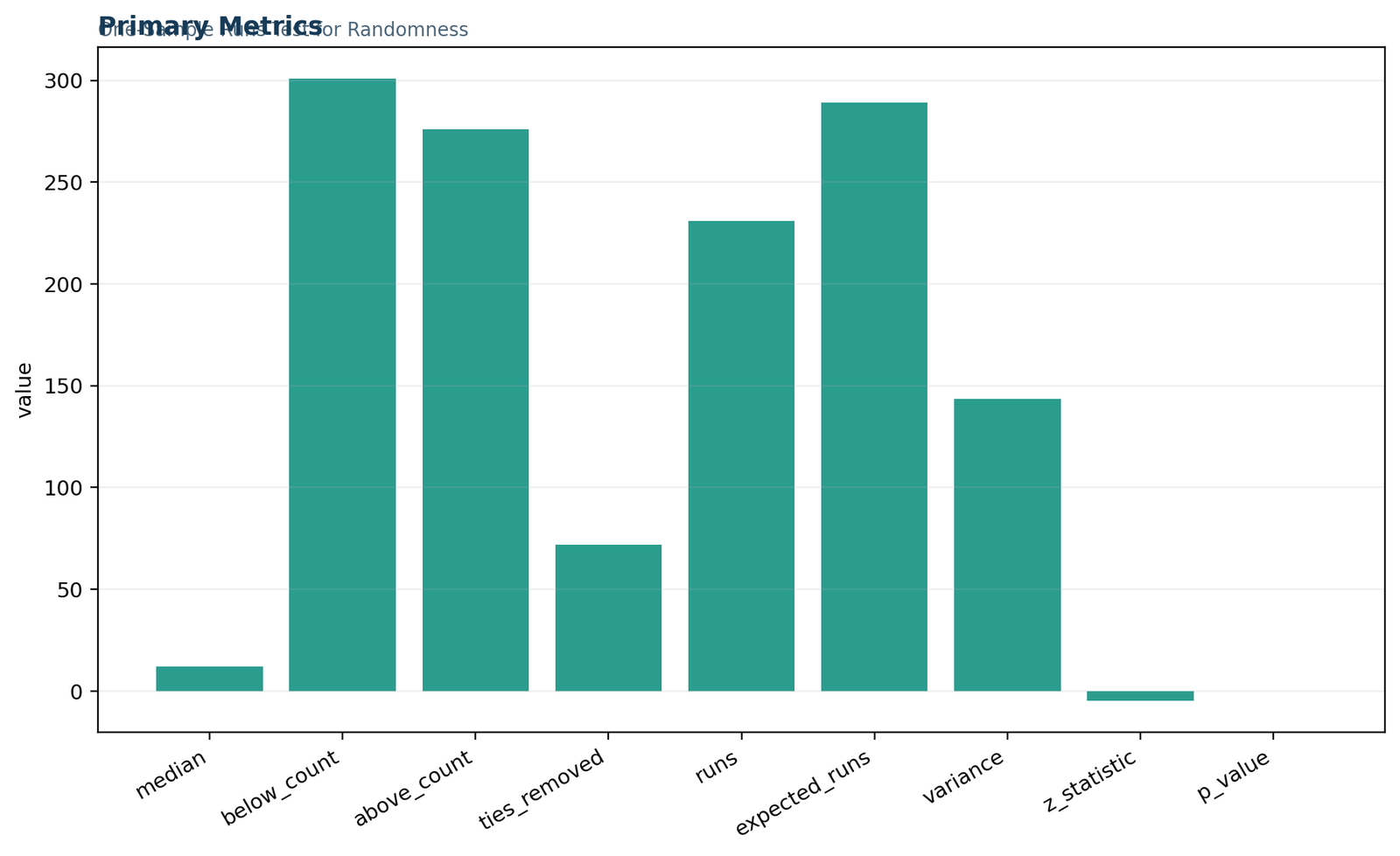
Python Chart 1: Primary metrics
The primary-metrics panel places the main quantities on one scale. Counts dominate visually, while z and p are necessarily compressed near zero. Read exact values from the accompanying result cards rather than from bar height alone.
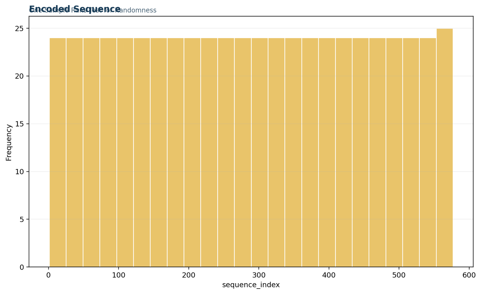
Python Chart 2: Encoded sequence coverage
This sequence-position panel confirms that the encoded analysis spans all 577 retained observations. Because it is an aggregated frequency-style display, individual zero-to-one transitions are better audited in the workbook Working sheet and the report table.
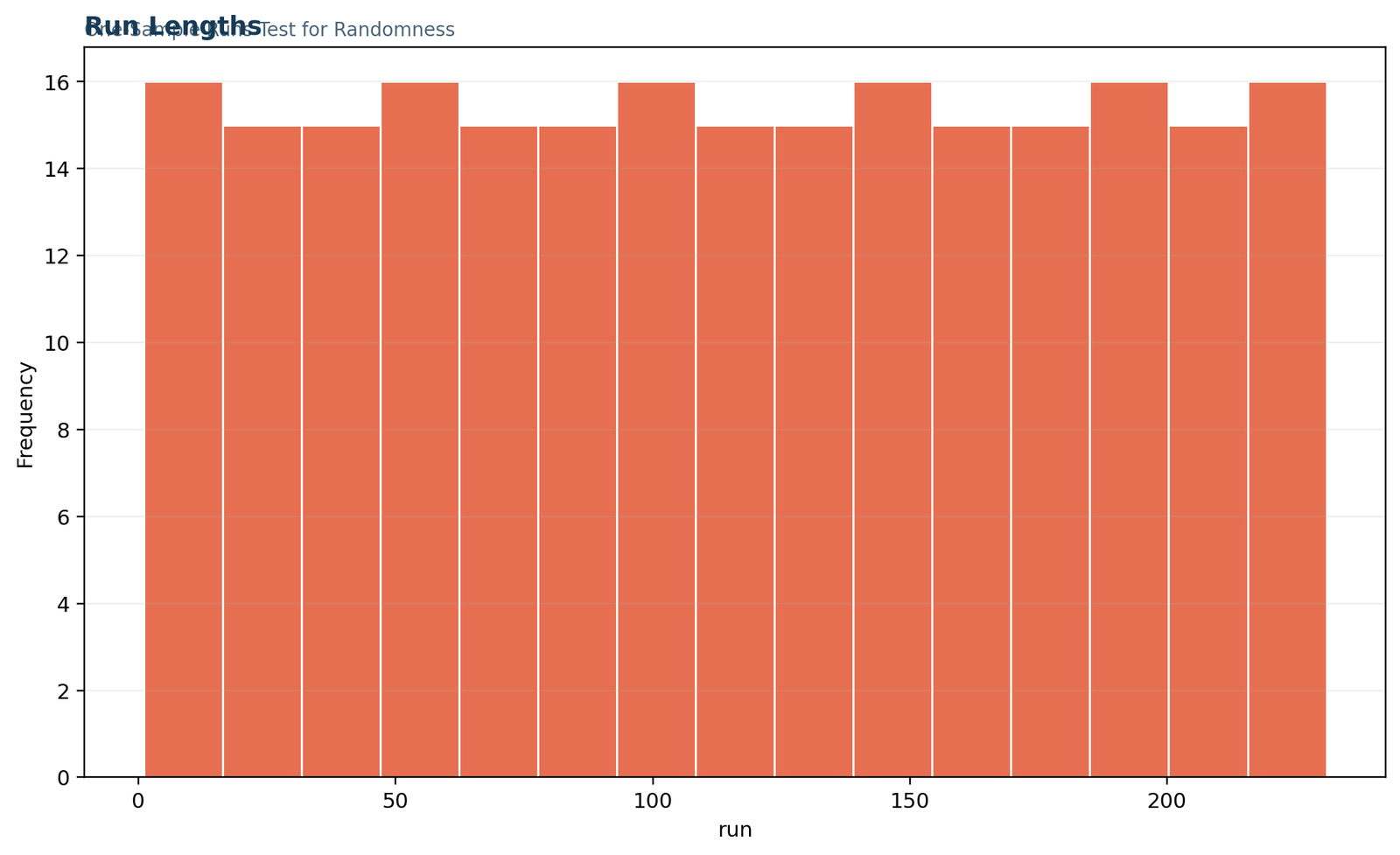
Python Chart 3: Run-length record coverage
The figure covers the full set of 231 run records. The exact lengths are not inferred from bar height in this aggregated view; the workbook confirms a median length of 1, a mean of 2.498 and a maximum of 30.
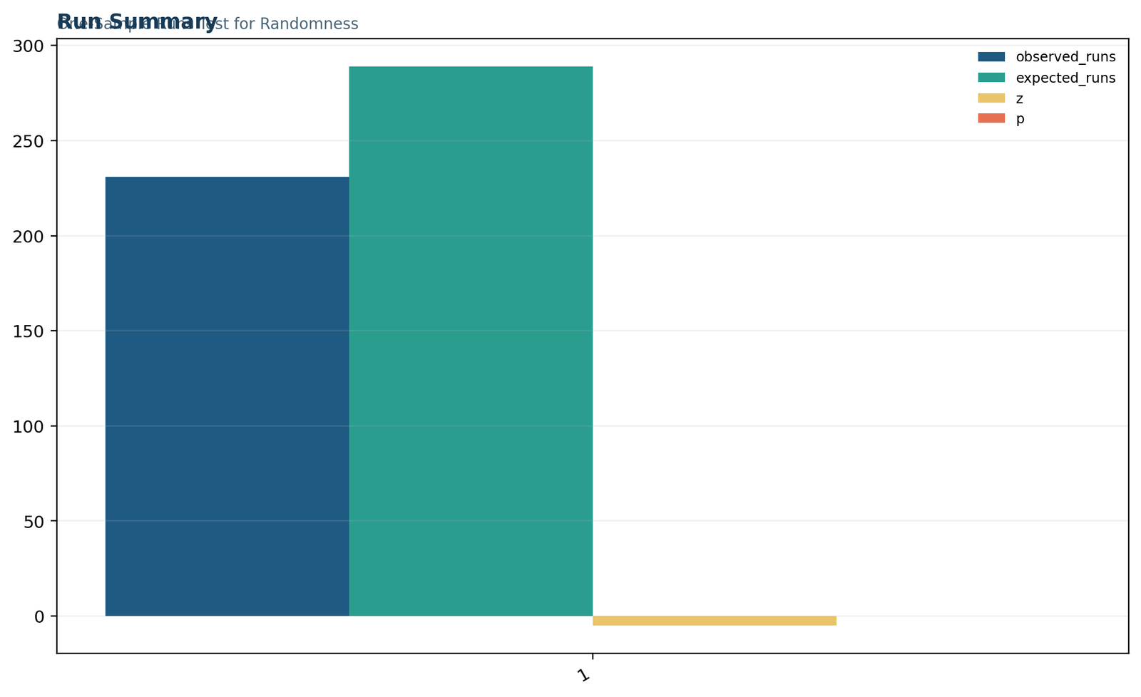
Python Chart 4: Observed versus expected runs
The principal contrast is clear: 231 observed runs are well below 288.958 expected runs. The negative z bar marks clustering, while the p-value is too small to be visually prominent on the shared count scale.
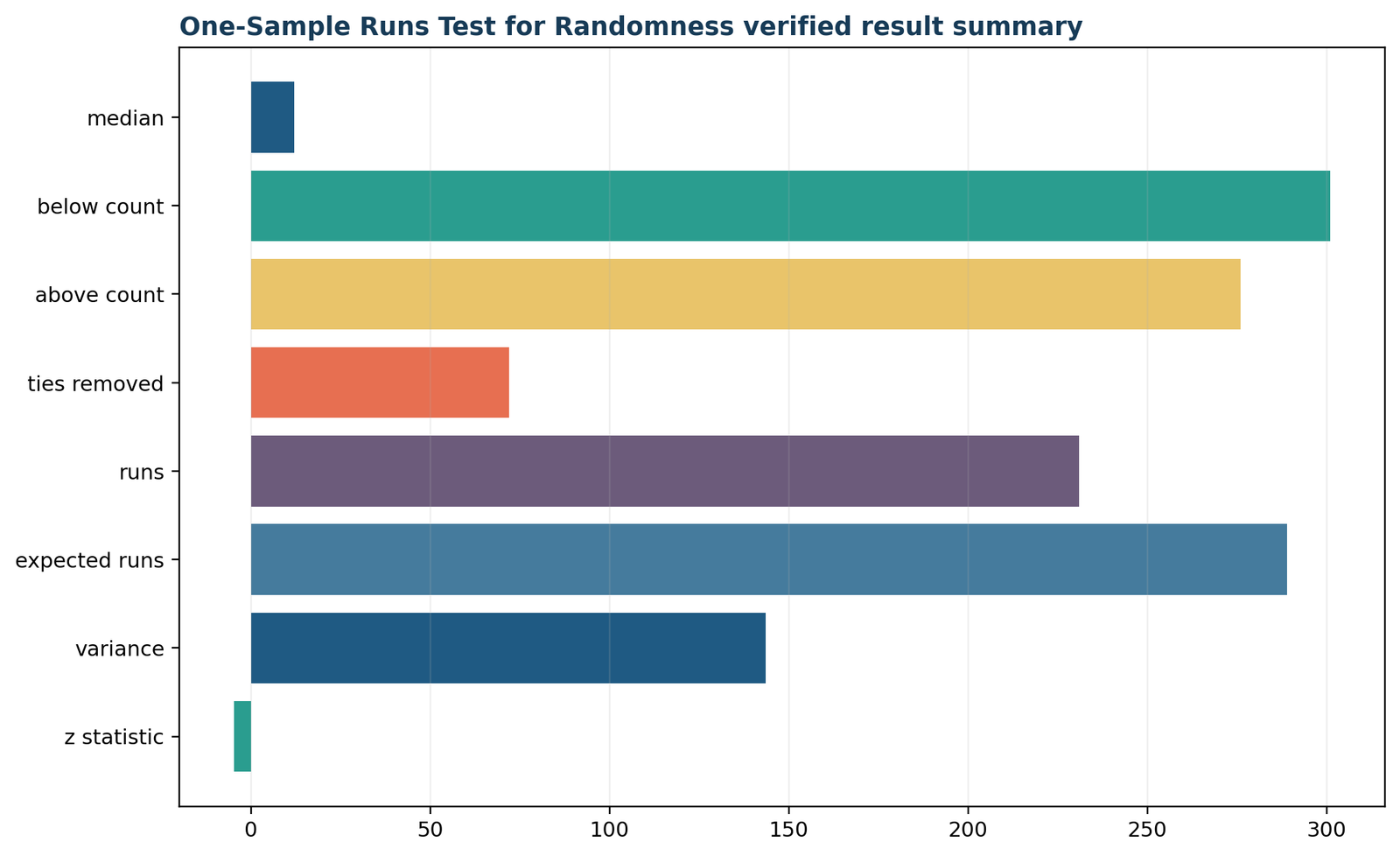
Python Chart 5: Verified result summary
The horizontal summary reproduces the median, below and above counts, removed ties, observed and expected runs, variance and z statistic. It provides a final visual cross-check of the formula-driven output.
Chart interpretation must respect scale. Combining counts near 300 with a p-value near one millionth makes the p bar nearly invisible. That does not imply p is missing; it reflects the very different units. The precise p-value should be reported numerically and, when graphed alone, on a logarithmic or transformed scale.
R charts for the runs test
The supplied R workflow independently reproduces the same calculated metrics and diagnostic coverage.
R Chart 1: Primary metrics
The R primary panel agrees with Python: median 12, 301 below, 276 above, 72 ties removed, 231 observed runs and 288.958 expected runs.
R Chart 2: Encoded sequence
The R sequence graphic spans the same retained observations. The binary coding rule is identical: 0 below the median, 1 above the median and median ties omitted.
R Chart 3: Run records
The run-record display covers all 231 runs. Exact run-length summaries should be read alongside the workbook because the figure emphasizes record coverage rather than individual length magnitudes.
R Chart 4: Run summary
The R comparison again shows a deficit of 57.958 runs. That deficit corresponds to z = −4.839 and a two-sided p-value of 1.305 × 10⁻⁶.
R Chart 5: Verified result summary
The final R panel is an independent visual confirmation that the same preprocessing and formulas were used in both languages.
Independent reproduction matters because a runs test can change materially with a different cutoff or tie policy. Agreement here is not merely agreement in the final p-value; Python and R also match on the median, retained counts, run total, expected value, variance and z statistic.
How to run the runs test in Python
A transparent implementation makes the tie rule and continuity-correction choice explicit.
Python libraries provide convenience functions, but a custom calculation is useful when an audit must reproduce a specific definition. The code below removes values exactly equal to the median, keeps all other observations in their original relative order and uses the uncorrected large-sample z formula from the workbook.
import numpy as np
from scipy.stats import norm# x must remain in the meaningful observed order.
x = np.asarray(g3_values, dtype=float)
cutoff = np.median(x)
# Remove values exactly equal to the median so the rule matches
# the audited workbook and the reproducible R calculation.
side = np.where(x < cutoff, 0,
np.where(x > cutoff, 1, np.nan))
side = side[~np.isnan(side)].astype(int)
n0 = np.sum(side == 0)
n1 = np.sum(side == 1)
N = n0 + n1
R = 1 + np.sum(side[1:] != side[:-1])
expected = 1 + (2 * n0 * n1) / N
variance = (2 * n0 * n1 * (2 * n0 * n1 - N)) / (N**2 * (N - 1))
z = (R - expected) / np.sqrt(variance)
p_value = 2 * norm.sf(abs(z))
print({
"median": cutoff,
"below": int(n0),
"above": int(n1),
"runs": int(R),
"expected": expected,
"variance": variance,
"z": z,
"p": p_value
})
The expected output is median = 12, below = 301, above = 276, runs = 231, expected = 288.9584055, variance = 143.4584808, z = −4.8389743 and p = 1.3051092e−06. Before running the code, verify that g3_values has not been sorted or grouped.
The Statsmodels one-sample function can discretize around a mean, median or numeric cutoff, and it offers a continuity-correction option. Convenience is valuable, but package defaults may not match a tie-removal protocol exactly. For a published analysis, print the package version and inspect the generated binary sequence. The broader Python data-analysis guide explains reproducible data loading and output practices.
len(side) == below + above, that sum(run_lengths) == len(side), and that recounting transitions gives the same R. These simple invariants catch silent sorting, tie and missing-data errors.How to run the runs test in R
Base R can reproduce every calculation without relying on a package-specific tie convention.
# g3 must be kept in its original, meaningful row order.
x <- as.numeric(g3)
cutoff <- median(x, na.rm = TRUE)# Remove observations exactly equal to the cutoff.
side <- ifelse(x < cutoff, 0,
ifelse(x > cutoff, 1, NA))
side <- side[!is.na(side)]
n0 <- sum(side == 0)
n1 <- sum(side == 1)
N <- n0 + n1
R <- 1 + sum(side[-1] != side[-length(side)])
expected <- 1 + 2 * n0 * n1 / N
variance <- 2 * n0 * n1 * (2 * n0 * n1 - N) /
(N^2 * (N - 1))
z <- (R - expected) / sqrt(variance)
p_value <- 2 * pnorm(-abs(z))
c(median = cutoff, below = n0, above = n1,
runs = R, expected = expected,
variance = variance, z = z, p = p_value)
The R vector must retain the source order. The expression comparing each label with its predecessor counts transitions; adding one includes the initial run. pnorm() converts the absolute z statistic to a two-sided normal-approximation p-value.
Package functions such as randtests::runs.test() are useful for standard analyses and may support a threshold argument and directional alternatives. Nevertheless, record the package version and read its documentation on ties, p-value method and plotting. The manual calculation above is included because it exactly mirrors the uploaded workbook. See the R data-analysis guide for project organization, scripts and result export.
For a small retained sequence, use an exact or permutation-based method rather than automatically trusting the asymptotic normal distribution. A permutation check can hold n₀ and n₁ fixed, randomly shuffle the binary labels many times and compare the simulated run count with R. This directly represents the conditional random-order null.
Runs test in SPSS
SPSS provides a native one-sample runs test, but its default treatment of values equal to the test value differs from the primary workbook rule.
* Native SPSS runs test using the sample median.
NPAR TESTS
/RUNS(MEDIAN)=G3
/STATISTICS=DESCRIPTIVES QUARTILES.* Tie-removed version matching the audited Python/R/Excel rule.
COMPUTE side_median = $SYSMIS.
IF (G3 < 12) side_median = 0.
IF (G3 > 12) side_median = 1.
VALUE LABELS side_median 0 'Below median' 1 'Above median'.
EXECUTE.
NPAR TESTS
/RUNS(0.5)=side_median.
Native SPSS output
With /RUNS(MEDIAN)=G3, SPSS reports test value 12, 301 cases below the test value and 348 cases greater than or equal to it. It retains all 649 cases, counts 253 runs, reports z = −5.592 and displays two-sided significance as .000.
Report that display as p < .001, never p = .000. SPSS’s result is valid for its documented grouping rule, but it is not numerically identical to the tie-removed Python/R/Excel analysis.
Matching the primary analysis
To reproduce the audited rule, create a binary variable with 0 below 12, 1 above 12 and system-missing for values equal to 12. Running the test at cutoff 0.5 then analyzes the same 577-label sequence.
Always verify the case counts in the output. A result showing 348 cases in the upper category indicates that the 72 median ties were retained there.
The supplied SPSS file also contains descriptive statistics: N = 649, mean = 11.91, standard deviation = 3.231, minimum = 0, median = 12 and maximum = 19. These validate the source data. The reported z of −5.592 still supports the same substantive conclusion—too few runs and significant clustering—but the numerical difference must not be presented as a software error. It arises from a different tie policy.
SPSS users can review the broader SPSS data-analysis guide for syntax, output management and reproducibility practices.
Runs test in Excel
A formula-driven workbook can expose every row-level label, transition and intermediate statistic.
Assume ordered G3 values are in A2:A650.

H2: =MEDIAN(A2:A650)

B2: =IF(A2<$H$2,0,IF(A2>$H$2,1,""))

D2: =FILTER(B2:B650,B2:B650<>"")

E2: =1

E3: =--(D3<>D2)   [copy down beside the spilled sequence]

H3: =COUNTIF(D2#,0)

H4: =COUNTIF(D2#,1)

H5: =H3+H4

H6: =SUM(E2:INDEX(E:E,ROWS(D2#)+1))

H7: =1+2*H3*H4/H5

H8: =2*H3*H4*(2*H3*H4-H5)/(H5^2*(H5-1))

H9: =(H6-H7)/SQRT(H8)

H10:=2*(1-NORM.S.DIST(ABS(H9),TRUE))
The uploaded Excel workbook separates raw input, working labels, calculations, diagnostics and reporting. This is preferable to placing every formula in one sheet because it preserves lineage. Yellow cells are fixed verified inputs and green cells are formulas. The Reporting sheet compares workbook results with an independent reference and shows zero or negligible floating-point differences.
Older Excel versions without FILTER can use a helper index to pull nonblank labels into a contiguous sequence, or they can count transitions while skipping ties with more complex formulas. The contiguous helper sequence is easier to audit. After building it, confirm that its row count equals 577 and that the number of 0 and 1 labels equals 301 and 276.
Excel’s NORM.S.DIST provides the large-sample p-value. It does not supply the exact small-sample run distribution automatically. For small sequences, use R, Python, dedicated software or a carefully implemented enumeration/permutation method. The general Excel analysis guide provides additional advice on formula auditing and reproducible workbook design.
Runs test assumptions
The method is distribution-free, but it still requires a defensible sequence, coding rule and null model.
The runs test does not assume a normal outcome, equal variances or interval-scale measurement. Binary outcomes can be analyzed directly. Numeric outcomes can be split around a cutoff. Nevertheless, dichotomization discards magnitude. If the size of deviations matters, a model using full numeric information may be more informative.
Extreme values usually have little direct impact when the median cutoff remains unchanged, because all above-median values receive the same label. But extreme values may matter if the mean is used as the cutoff. Inspect outliers, a box plot and the interquartile range before deciding which threshold is substantively appropriate.
Runs test diagnostics and interpretation
Good reporting separates the statistical pattern from possible substantive explanations.
Direction and magnitude
The observed deficit is 57.958 runs, or 20.1% below the null expectation. The optional standardized descriptive index |z|/√N is 0.201. This can communicate magnitude, but it is not a universally standardized runs-test effect size and should not replace R, E(R), z and p.
The sequence contains many singleton runs, yet the overall run count is low because several long stretches offset them. This illustrates why a histogram or mean run length alone cannot replace the formal conditional calculation.
Sensitivity checks
Repeat the analysis with scientifically reasonable cutoff rules established in advance, not as a significance hunt. Compare tie removal with tie assignment, exact with asymptotic p-values and corrected with uncorrected z values. A robust conclusion should retain its broad direction.
For the worked example, native SPSS and the tie-removed calculation differ numerically but both produce strongly negative z statistics and reject randomness.
Inspect the encoded sequence directly. A simple line of 0/1 labels, a cumulative count, a run-length plot and a table of the longest runs can reveal whether rejection is driven by one large cluster or by broad persistence. The present sequence’s maximum run length of 30 is notable, but the inferential result uses all 231 runs.
Consider process explanations: chronological cohorts, school grouping, data-entry batches, sorting inherited from the source file or actual serial dependence. If the sequence order is arbitrary database order, a significant result may describe file organization rather than a substantive phenomenon. This is why metadata about row order are as important as the p-value.
For ordered quantitative residuals, supplement the runs test with an autocorrelation analysis or Durbin–Watson diagnostic. For a prespecified monotone ordered alternative across repeated conditions, Page’s trend test answers a different question and uses within-block ranks.
Runs test calculator workflow and critical-value logic
A reliable calculator must expose the coding choices that determine the sequence instead of accepting only a final run count.
Inputs a runs test calculator needs
A defensible runs test calculator begins with the ordered observations or an already validated binary sequence. For numeric observations it also needs the cutoff rule: sample median, sample mean, zero, a target value or a user-entered threshold. It must ask what to do with values exactly equal to the cutoff. Those values can be removed, assigned to the lower group, assigned to the upper group or handled under a specialized tie convention.
Entering only n₀, n₁ and R is enough to reproduce the asymptotic formula, but it is not enough to verify that R was counted correctly. A high-quality runs test calculator should therefore display the encoded sequence, mark every run start and list the run lengths. The sequence preview catches accidental sorting and inconsistent tie treatment before they become a published result.
Outputs a runs test calculator should show
The essential outputs are n₀, n₁, retained N, observed runs R, expected runs E(R), run-count variance, standard deviation, z statistic and p-value. The output should identify whether the alternative is two-sided, clustering or alternation. It should also state whether an exact distribution, a normal approximation or a continuity-corrected approximation was used.
For this worked runs test, a verified calculator should return n₀ = 301, n₁ = 276, N = 577, R = 231, E(R) = 288.9584, variance = 143.4585, z = −4.8390 and two-sided p = 1.305 × 10⁻⁶. A different result is a signal to inspect the median ties or continuity correction.
Step-by-step runs test calculator checklist
Traditional critical-value tables list lower and upper rejection limits for combinations of n₀ and n₁. They remain useful for teaching and manual checks, but software p-values are more flexible. A table must match the intended significance level and one- or two-sided alternative. It may also be limited to small category counts. Never compare an asymptotic z result with a table that uses a different tail definition and assume disagreement means an error.
For an exact runs test, the probability of each possible run count is obtained from the number of binary arrangements with that run count, conditional on n₀ and n₁. The combinatorial formulas differ for even and odd R. Modern software can enumerate or compute these probabilities directly. A permutation implementation reaches the same null concept by repeatedly shuffling the fixed labels and recounting runs.
When N is large, the z approximation is usually convenient. The worked runs test has both category counts above 250, so asymptotic inference is stable. The p-value is also far below .05, making the substantive decision insensitive to minor continuity-correction differences. The more consequential choice is whether the 72 median ties are removed or assigned to a category.
Common runs test mistakes and how to prevent them
Most serious errors occur before the formula is evaluated: order is changed, ties are hidden or the wrong runs procedure is selected.
Sorting the outcome
Sorting places all low labels together and all high labels together, creating two runs or a similarly tiny number. That is not evidence discovered by a runs test; it is an artifact created by preprocessing. Freeze and document the order before analysis.
Ignoring cutoff ties
A result cannot be reproduced when the report says only “median split.” State whether equality belongs above, below or neither. In this example, tie removal changes the retained N from 649 to 577 and the run count from the native SPSS value of 253 to 231.
Confusing one- and two-sample tests
The one-sample runs test examines randomness in one ordered binary sequence. The two-sample Wald–Wolfowitz procedure pools two samples, orders their values and examines mixing. Their inputs and null hypotheses are different.
Reporting p = .000
Software rounds very small values. A displayed .000 is not a probability of exactly zero. Report p < .001 or a higher-precision value such as 1.305 × 10⁻⁶.
Using arbitrary row order
A database export may be ordered by school, identifier, batch or storage history. A significant runs test then describes that file order unless the order has substantive meaning. Explain the sequence source.
Calling significance causation
Rejected randomness does not identify a mechanism. Clustering may arise from cohorts, sorting variables, process shifts, omitted structure or genuine serial dependence. Follow-up investigation is required.
Another frequent mistake is to interpret category balance as randomness. In the worked data, 301 below-median and 276 above-median observations are reasonably balanced, but balance says nothing about arrangement. The same counts can form a highly alternating sequence, a highly clustered sequence or countless intermediate sequences. The runs test focuses on arrangement conditional on those counts.
Conversely, analysts sometimes treat every visually noticeable streak as significant. Long runs are expected occasionally, especially in large sequences. The formal runs test evaluates the total run count against its conditional distribution. A longest-run analysis is a separate diagnostic and may require its own null distribution.
Do not use a runs test as a general substitute for a model. If measurements have seasonality, trends, known interventions or unequal time gaps, a time-series or regression model can represent those structures directly. The runs test is most useful as a simple omnibus order diagnostic or when only binary labels are meaningful.
Continuity correction is another source of unexplained differences. Some implementations adjust the numerator by 0.5 for small samples; others do not. The correction should move the statistic toward zero. Record the setting. In this worked runs test, the supplied Python, R and Excel analyses intentionally use the uncorrected formula, and the large retained N makes this choice secondary to tie handling.
Finally, avoid excessive precision without context. Report enough digits to reproduce the result—R = 231, E(R) = 288.958, z = −4.839 and p = 1.305 × 10⁻⁶—but interpret the pattern in plain language. The practical message is that the sequence has substantially fewer runs than expected, indicating clustering of grades on the same side of the median.
Runs test compared with related methods
Tests that use the word “run,” order, rank or randomness may target very different null hypotheses.
| Method | Main question | Uses order? | Key distinction |
|---|---|---|---|
| One-sample runs test | Are two labels randomly arranged in one sequence? | Yes | Counts same-label blocks around a cutoff |
| Two-sample Wald–Wolfowitz runs test | Do two independent samples appear intermixed after pooling and sorting? | Order of pooled values | Tests distributional separation between groups |
| Sign test | Is a population median equal to a target? | No | Uses signs but ignores their sequence; see sign test |
| Binomial test | Does the proportion of one label equal a hypothesized probability? | No | Uses counts only; see binomial test |
| Chi-square goodness of fit | Do category frequencies match expected proportions? | No | Ignores adjacency; see chi-square goodness of fit |
| Durbin–Watson test | Is there first-order autocorrelation in regression residuals? | Yes | Uses residual magnitudes and a regression context |
| Page’s trend test | Do related conditions follow a prespecified monotone order? | Ordered conditions | Repeated blocks and ranks, not sequence randomness |
For three or more independent groups, the Kruskal–Wallis test compares rank distributions. For repeated conditions, the Friedman test or Quade test may be appropriate. For two independent samples with a robust relative-effect target, review the Brunner–Munzel test. For two-sample scale, see the Ansari–Bradley test. None of these substitutes for a runs test when the primary estimand is randomness of a single ordering.
The phrase “Wald–Wolfowitz runs test” is sometimes used for both the one-sample randomness test and the two-sample pooled-order test. State the design explicitly to avoid ambiguity. This article and workbook use the one-sample above/below cutoff runs test for randomness.
How to report the runs test in APA style
Report the sequence definition, cutoff, tie rule, category counts, run count, approximation and directional interpretation.
APA-style results paragraph
“A two-sided one-sample runs test examined whether final grades occurred in a random row order relative to the sample median. The median was 12. Observations equal to the median were removed, leaving 301 below-median and 276 above-median grades (N = 577). The sequence contained 231 runs, fewer than the 288.96 runs expected under random ordering, z = −4.84, p < .001. Thus, the null hypothesis of random ordering was rejected; grades on the same side of the median clustered more than expected.”
When space allows, report the exact p-value as p = 1.31 × 10⁻⁶. In ordinary APA prose, p < .001 is acceptable and easier to read. Do not write p = .000. Include the original source count of 649 and the removal of 72 median ties in a methods or data-preparation paragraph.
For SPSS’s native result, use a separate sentence: “SPSS assigned values equal to the median to the greater-than-or-equal category and retained all 649 cases, yielding 253 runs, z = −5.59, p < .001.” Do not place the SPSS and tie-removed statistics in one unlabeled table because readers may assume they are directly interchangeable.
Effect-size reporting is optional because there is no single universally adopted runs-test effect measure. When reporting |z|/√N = 0.20144913603753983322, label it as a standardized descriptive index and explain the denominator. Emphasize the observed and expected run counts because they are directly interpretable.
Runs test downloads and reproducibility files
Download the verified reports and formula-driven workbook used for this guide.
Reproducibility requires more than a downloadable result. Preserve the raw order, document the meaning of that order, record the cutoff and tie rule, keep software versions, and retain code or formulas that reconstruct every reported statistic. The supplied workbook’s separation of input and calculations supports this audit trail.
Runs test frequently asked questions
Concise answers to common interpretation, formula and software questions.
What is a runs test?
A runs test is a nonparametric procedure for evaluating whether two labels occur in a random order. A run is an uninterrupted sequence of identical labels. The one-sample version commonly codes observations above and below a median or another cutoff.
What does a negative z mean?
A negative z means fewer runs were observed than expected. That direction indicates clustering or persistence of identical labels. A positive z indicates more alternation than expected.
Why were values equal to the median removed?
The primary analysis used a strict below-versus-above definition. Equal values do not belong to either strict category, so they were removed while preserving the relative order of all remaining observations. Other software may assign ties to one side; that policy must be reported.
Why does SPSS give a different result?
Native SPSS groups cases greater than or equal to the test value together. In this example it keeps the 72 median ties in the upper category, producing 253 runs instead of 231. Both analyses reject randomness, but they analyze different binary sequences.
Is p = .000 a valid report?
No. A display of .000 means the rounded p-value is below the displayed precision. Report p < .001 or an exact value from a higher-precision calculation.
Does the runs test require normal data?
No. It does not assume a normal outcome distribution. It does require a meaningful sequence, a defensible binary coding rule and appropriate handling of ties and small samples.
Can the test detect autocorrelation?
It can detect nonrandom clustering or alternation in a binary-coded sequence and is sometimes used as a general independence diagnostic. It does not estimate a lag-specific autocorrelation coefficient. Dedicated time-series tests may provide more detailed information.
What is the runs test calculator formula?
Calculate E(R) = 1 + 2n₀n₁/N and Var(R) = 2n₀n₁(2n₀n₁ − N)/[N²(N − 1)], then z = [R − E(R)]/√Var(R). Use the standard normal distribution for the large-sample p-value.
Should I use the mean or median cutoff?
Use the cutoff that best represents the research question. The median is robust and often balances categories. Zero, a target or a specification limit may be more meaningful for residuals or process data. Specify the choice before inspecting the sequence.
What if the sequence has many ties?
Many ties can substantially change the retained sample and the arrangement. Report the tie count, conduct a justified sensitivity analysis and avoid presenting results from different tie rules as though they were identical.
Can I sort the data before the test?
No. Sorting by the outcome almost guarantees long blocks and invalidates the intended randomness question. Use the original meaningful order.
What should be reported?
Report the order definition, cutoff, tie rule, n₀, n₁, retained N, observed runs, expected runs, z, p-value, alternative hypothesis, approximation or exact method and substantive direction.