
Two binary variables, latent-normal thresholds, phi comparison, likelihood profile and Excel worked result
Tetrachoric Correlation: Formula, Interpretation, SPSS, Python, R and Excel Guide
Tetrachoric Correlation estimates the latent correlation between two binary variables when both observed binary variables are assumed to come from underlying continuous latent traits. It is often used with yes/no variables, pass/fail variables, symptom present/absent variables, item response data, screening questions and dichotomized survey items. This guide explains the 2×2 table, latent thresholds, phi comparison, Digby approximation, maximum-likelihood tetrachoric estimate, likelihood profile, Python charts, R validation charts, SPSS output, Excel formulas, APA reporting and common mistakes.
Quick Answer: Tetrachoric Correlation Result
The worked example estimates the latent association between higher education intention and internet access. The X variable is higher, coded yes = 1 and no / all other = 0. The Y variable is internet, coded yes = 1 and no / all other = 0. Both variables are binary, so the observed 2×2 table can be summarized with phi, odds ratio, Yule Q and tetrachoric correlation.
The verified observed table is: 451 students with higher=yes and internet=yes, 129 with higher=yes and internet=no, 47 with higher=no and internet=yes, and 22 with higher=no and internet=no. The exact MLE tetrachoric correlation is ρ = 0.152843. The 95% confidence interval is -0.0180 to 0.3237. The observed phi coefficient is 0.070345, and the Digby tetrachoric approximation is 0.194731.
Final interpretation: The data show a small positive latent association between higher education intention and internet access. Students who intended to pursue higher education were somewhat more likely to report internet access, but the confidence interval crosses zero and the chi-square p-value is above .05. Therefore, report the result cautiously rather than claiming a clearly significant association.
Important reporting point: Phi coefficient measures the observed association between two 0/1 variables. Tetrachoric correlation estimates the latent association behind those binary variables. In this example, phi is 0.0703, while exact MLE tetrachoric rho is 0.1528. The tetrachoric value is larger because it assumes the yes/no variables are thresholded versions of underlying continuous traits.
Table of Contents
- What Is Tetrachoric Correlation?
- When Should You Use Tetrachoric Correlation?
- Tetrachoric vs Phi vs Polychoric vs Point Biserial
- Tetrachoric Correlation Formula Logic
- Null and Alternative Hypotheses
- Dataset and Binary Variables Used
- Observed 2×2 Table
- Verified Tetrachoric Results
- Expected Counts and Residual Context
- Python Chart-by-Chart Interpretation
- R Chart-by-Chart Interpretation
- SPSS Output Interpretation
- Excel Worked File Explanation
- Python, R, SPSS and Excel Workflows
- Code Blocks and Excel Formulas
- Assumptions and Data Checks
- How to Report Tetrachoric Correlation
- Common Mistakes
- Downloads and Resources
- Related Statistical Guides
- FAQs About Tetrachoric Correlation
What Is Tetrachoric Correlation?
Tetrachoric Correlation estimates the correlation between two unobserved continuous latent variables when both observed variables are binary. The observed binary responses are treated as thresholded outcomes. In other words, each yes/no variable is assumed to be a cut version of a hidden continuous tendency.
For example, the observed variable higher records whether a student wants higher education. The observed variable internet records whether a student has internet access. Both are binary yes/no variables. Tetrachoric correlation asks: if these yes/no responses came from hidden continuous tendencies, how strongly would those hidden tendencies be correlated?
This is different from the Phi Coefficient. Phi is the Pearson correlation between two observed 0/1 variables. Tetrachoric correlation is a model-based latent correlation. It usually becomes larger than phi when the binary variables are unbalanced or when the latent-threshold assumption suggests a stronger underlying association than the raw table shows.
Tetrachoric Correlation connects naturally with Phi Coefficient, Cross Tabulation, Contingency Coefficient, Polychoric Correlation, Point Biserial Correlation, Correlation in Python, Correlation in R, Correlation in SPSS, Correlation in Excel, Effect Size and p-value.
Simple definition: Tetrachoric Correlation estimates the latent correlation behind two binary variables under a bivariate-normal threshold model.
When Should You Use Tetrachoric Correlation?
Use Tetrachoric Correlation when both variables are binary and you believe each binary variable represents a cut point on an underlying continuous or latent trait. It is common in psychometrics, survey research, item analysis, health screening, test items, educational data, social science and binary response modeling.
| Situation | Use Tetrachoric? | Reason | Example |
|---|---|---|---|
| Both variables are binary yes/no | Yes, if latent threshold assumption is reasonable | Tetrachoric estimates the hidden correlation behind two binary outcomes. | higher yes/no by internet yes/no. |
| Both variables are dichotomized from underlying traits | Yes | This is the strongest theoretical use case. | high anxiety yes/no by high stress yes/no. |
| Both variables are test items scored correct/incorrect | Often yes | Item responses may reflect latent ability traits. | item 1 correct by item 2 correct. |
| Both variables are observed binary but no latent assumption is intended | Use phi or odds ratio | Phi describes the observed 2×2 association directly. | internet yes/no by pass/fail as purely observed categories. |
| Both variables are ordinal with more than two categories | No | Use polychoric correlation. | Dalc by Walc with 1 to 5 categories. |
| One variable is binary and one is continuous | No | Use point-biserial correlation. | sex code by G3 score. |
| One variable is ordinal and one is continuous | No | Use polyserial correlation. | studytime category by G3 score. |
The worked example is suitable for teaching because both variables are binary. The main caution is that the latent-normal threshold assumption must be explained. If a researcher only wants the observed 2×2 association, phi, chi-square, odds ratio and Yule Q may be more direct.
Tetrachoric vs Phi vs Polychoric vs Point Biserial
Different correlation names are used because variables can be continuous, binary, ordinal or latent. The correct method depends on the scale of both variables and the research assumption.
| Measure | Use It When | What It Estimates | Example |
|---|---|---|---|
| Tetrachoric Correlation | Both observed variables are binary and assumed to be thresholded latent traits. | Latent bivariate-normal correlation. | higher yes/no by internet yes/no. |
| Phi Coefficient | Both variables are binary and you want the observed 0/1 association. | Pearson correlation on observed binary codes. | higher code by internet code. |
| Polychoric Correlation | Both variables are ordinal with more than two categories. | Latent correlation behind ordinal categories. | Dalc by Walc. |
| Polyserial Correlation | One variable is ordinal and one variable is continuous. | Latent ordinal-continuous association. | studytime by G3. |
| Point Biserial Correlation | One variable is true binary and one variable is continuous. | Observed binary-continuous correlation. | sex code by G3. |
| Odds Ratio | Both variables are binary and comparison is framed in odds. | Ratio of positive outcome odds across groups. | internet access odds by higher education intention. |
Practical rule: Use phi and chi-square to describe the observed 2×2 table. Use tetrachoric correlation when you want a latent correlation estimate and the bivariate-normal threshold assumption is reasonable.
Tetrachoric Correlation Formula Logic
Tetrachoric Correlation is usually estimated by maximum likelihood. The method assumes two hidden continuous variables, X* and Y*, with a bivariate normal distribution. Each observed binary variable is produced by cutting its hidden variable at a threshold.
The thresholds are estimated from the marginal proportions. In this workbook, P(X=1) for higher=yes is 0.893683, and P(Y=1) for internet=yes is 0.767334. The corresponding latent thresholds are -1.246353 for X and -0.730096 for Y.
The maximum-likelihood estimate finds the value of ρ that best reproduces the observed 2×2 table probabilities under the threshold model. In this workbook, the exact MLE is 0.152843. The workbook also reports a closed-form Digby approximation of 0.194731, which is useful for comparison but not the primary exact estimate.
Phi Formula for Comparison
The observed phi coefficient is calculated directly from the 2×2 table:
For this table, phi is 0.070345. Phi is smaller than the tetrachoric estimate because phi is the raw observed binary association, while tetrachoric estimates latent association.
Null and Alternative Hypotheses
The hypothesis test asks whether the population association between the two binary variables is zero. Depending on the reporting focus, the hypothesis may be stated for the latent tetrachoric correlation or for the observed 2×2 association.
| Statement | Hypothesis | Meaning |
|---|---|---|
| Latent null hypothesis | H0: ρtet = 0 | The hidden latent variables behind higher and internet are not associated. |
| Latent alternative hypothesis | H1: ρtet ≠ 0 | The hidden latent variables are associated. |
| Observed table null hypothesis | H0: variables are independent | The observed 2×2 table shows no association. |
| Observed table alternative | H1: variables are associated | The observed 2×2 table shows association. |
| Workbook context | χ² p = 0.073121 | Observed table evidence is not below .05. |
Decision: The latent estimate is positive, but the 95% CI crosses zero and the chi-square p-value is 0.073121. At α = .05, the safest report is: small positive latent association, not clearly statistically significant in the observed table context.
Dataset and Binary Variables Used
The analysis uses the student performance dataset with 649 valid observations. The workbook selects two binary variables: higher and internet. Both are coded so that yes = 1 and all other observed categories are coded 0.
| Variable | Role | Positive Category | Reference Category | Valid Cases |
|---|---|---|---|---|
| higher | X binary variable | yes coded 1 | no / all other coded 0 | 649 |
| internet | Y binary variable | yes coded 1 | no / all other coded 0 | 649 |
Before interpreting the coefficient, it is helpful to review Cross Tabulation, Phi Coefficient, Effect Size, p-value, Confidence Interval, Frequency Distribution and Null and Alternative Hypothesis.
Observed 2×2 Table
The observed 2×2 table is the foundation of the tetrachoric analysis. It shows how many students fall into each combination of higher education intention and internet access.
| Observed Table | Y=1 internet yes | Y=0 internet no | Row Total | Row % Internet Yes |
|---|---|---|---|---|
| X=1 higher yes | 451 | 129 | 580 | 77.7586% |
| X=0 higher no | 47 | 22 | 69 | 68.1159% |
| Column total | 498 | 151 | 649 | 76.7334% |
The row percentage pattern is positive. Students with higher=yes have internet=yes at 77.76%, while students with higher=no have internet=yes at 68.12%. The difference is about 9.64 percentage points. This produces a positive association, but the difference is not large enough to produce a strong observed-table result.
Verified Tetrachoric Results
The table below summarizes the verified values from the uploaded Excel workbook.
| Measure | Verified Value | Interpretation |
|---|---|---|
| n11 | 451 | higher=yes and internet=yes. |
| n10 | 129 | higher=yes and internet=no. |
| n01 | 47 | higher=no and internet=yes. |
| n00 | 22 | higher=no and internet=no. |
| Total N | 649 | Total valid cases. |
| P(X=1) | 0.893683 | Proportion higher=yes. |
| P(Y=1) | 0.767334 | Proportion internet=yes. |
| Observed P(X=1,Y=1) | 0.694915 | Joint positive proportion. |
| Threshold X | -1.246353 | Latent normal threshold for higher=yes. |
| Threshold Y | -0.730096 | Latent normal threshold for internet=yes. |
| Phi coefficient | 0.070345 | Observed 0/1 binary correlation. |
| Continuity-corrected odds ratio | 1.651494 | Higher=yes group has higher odds of internet=yes. |
| Yule Q | 0.245708 | Odds-ratio-based association measure. |
| Digby tetrachoric approximation | 0.194731 | Closed-form approximation. |
| Exact MLE tetrachoric correlation | 0.152843 | Primary latent correlation estimate. |
| Standard error | 0.087188 | Observed-information approximation. |
| 95% CI lower | -0.018043 | Lower confidence limit. |
| 95% CI upper | 0.323728 | Upper confidence limit. |
| Chi-square statistic | 3.211522 | Observed 2×2 association context. |
| Chi-square p-value | 0.073121 | Not below .05. |
The key result is that all association measures are positive, but small. The exact MLE tetrachoric estimate is larger than phi, but the uncertainty interval crosses zero. Therefore, the best conclusion is cautious: the data suggest a small positive latent association, but the evidence is not strong enough for a clear .05-level observed-table conclusion.
Expected Counts and Residual Context
Expected counts under independence help explain the chi-square result. They show what the 2×2 table would look like if higher and internet were independent.
| Expected Table | Y=1 Internet Expected | Y=0 Internet Expected | Row Total | Expected Row % Internet Yes |
|---|---|---|---|---|
| X=1 higher expected | 445.0539 | 134.9461 | 580 | 76.7334% |
| X=0 higher expected | 52.9461 | 16.0539 | 69 | 76.7334% |
The observed count for higher=yes and internet=yes is 451, slightly above the expected count of 445.05. The observed count for higher=no and internet=no is 22, above the expected count of 16.05. These deviations support a positive relationship, but the deviations are not large enough to produce a chi-square p-value below .05.
Python Chart-by-Chart Interpretation
The Python report includes five visuals: a 2×2 frequency heatmap, binary marginal distributions, phi versus tetrachoric comparison, likelihood profile, and method report card. These charts explain the observed table, the latent estimate, and the uncertainty around the final result.
Python Chart 1: Tetrachoric 2×2 Frequency Heatmap
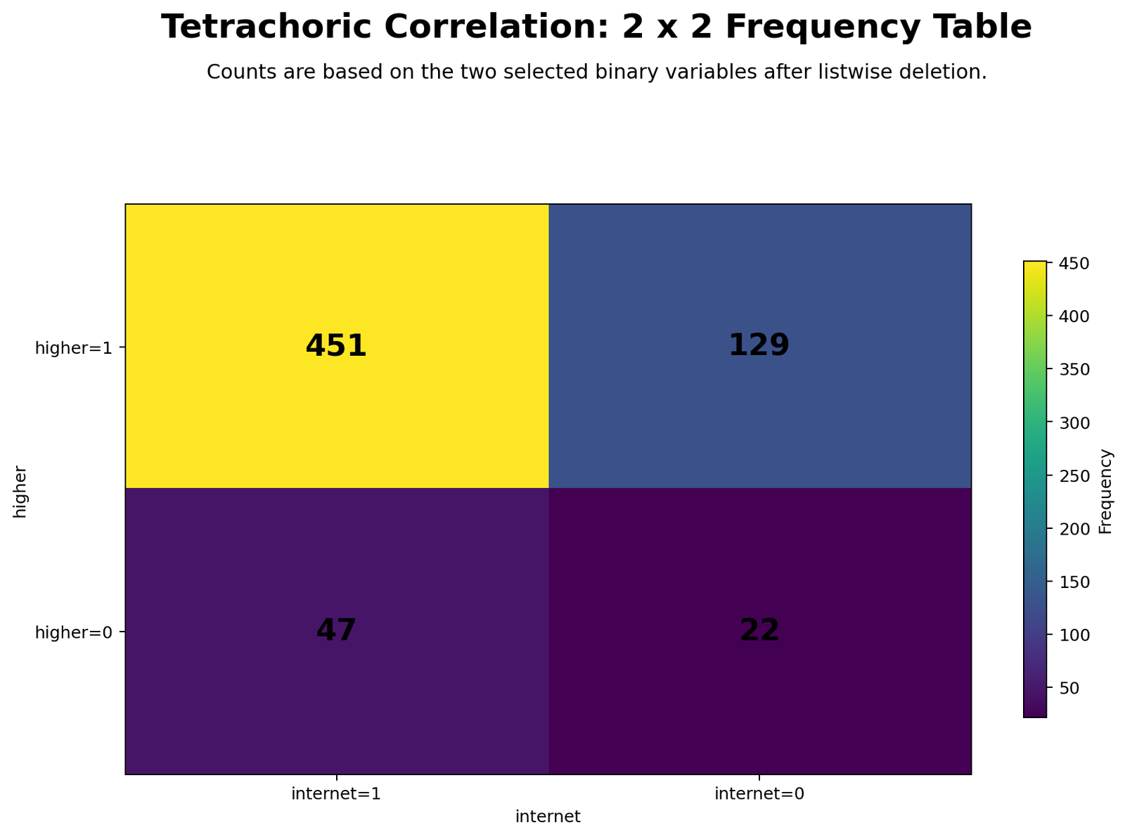
The heatmap shows the four observed cells in the 2×2 table. The largest cell is higher=yes and internet=yes, with 451 students. This is expected because both yes categories are common in the dataset. The higher=yes and internet=no cell has 129 students, the higher=no and internet=yes cell has 47 students, and the higher=no and internet=no cell has 22 students.
The visual pattern is positive because the internet=yes percentage is higher among students with higher=yes than among students with higher=no. However, the table is also highly unbalanced because most students answered higher=yes. This imbalance is one reason why the phi coefficient is small and why the tetrachoric estimate should be interpreted cautiously.
Python Chart 2: Binary Marginal Distributions
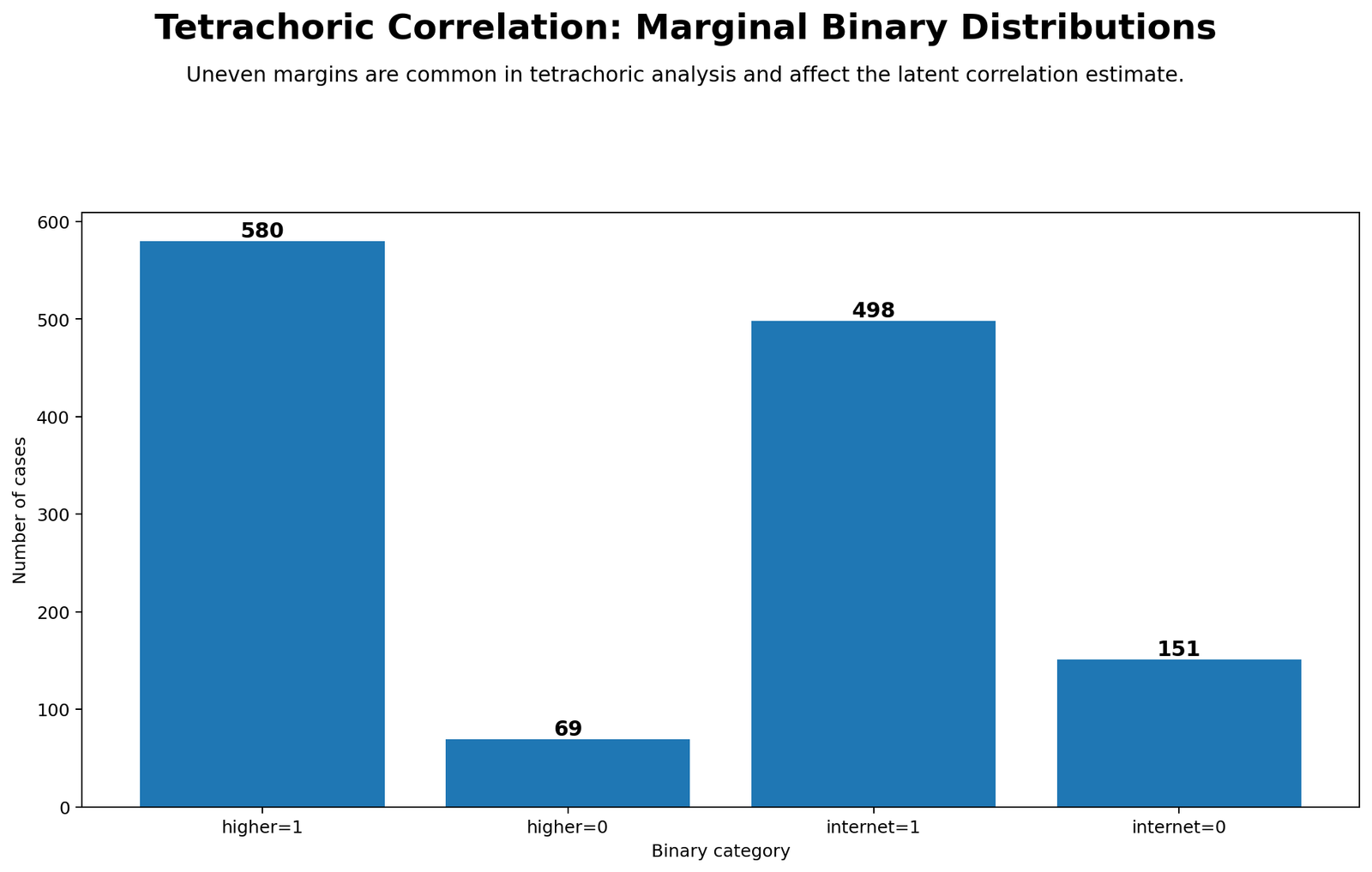
The marginal distribution chart shows that higher=yes is very common, with 580 of 649 observations. Internet=yes is also common, with 498 of 649 observations. These high positive-category proportions create asymmetric margins.
This chart matters because tetrachoric correlation is based on latent thresholds derived from the marginal proportions. When margins are unbalanced, the latent thresholds move away from zero. In this workbook, the threshold for higher is -1.2464 and the threshold for internet is -0.7301. These thresholds are part of why the tetrachoric estimate differs from phi.
Python Chart 3: Phi vs Tetrachoric Comparison
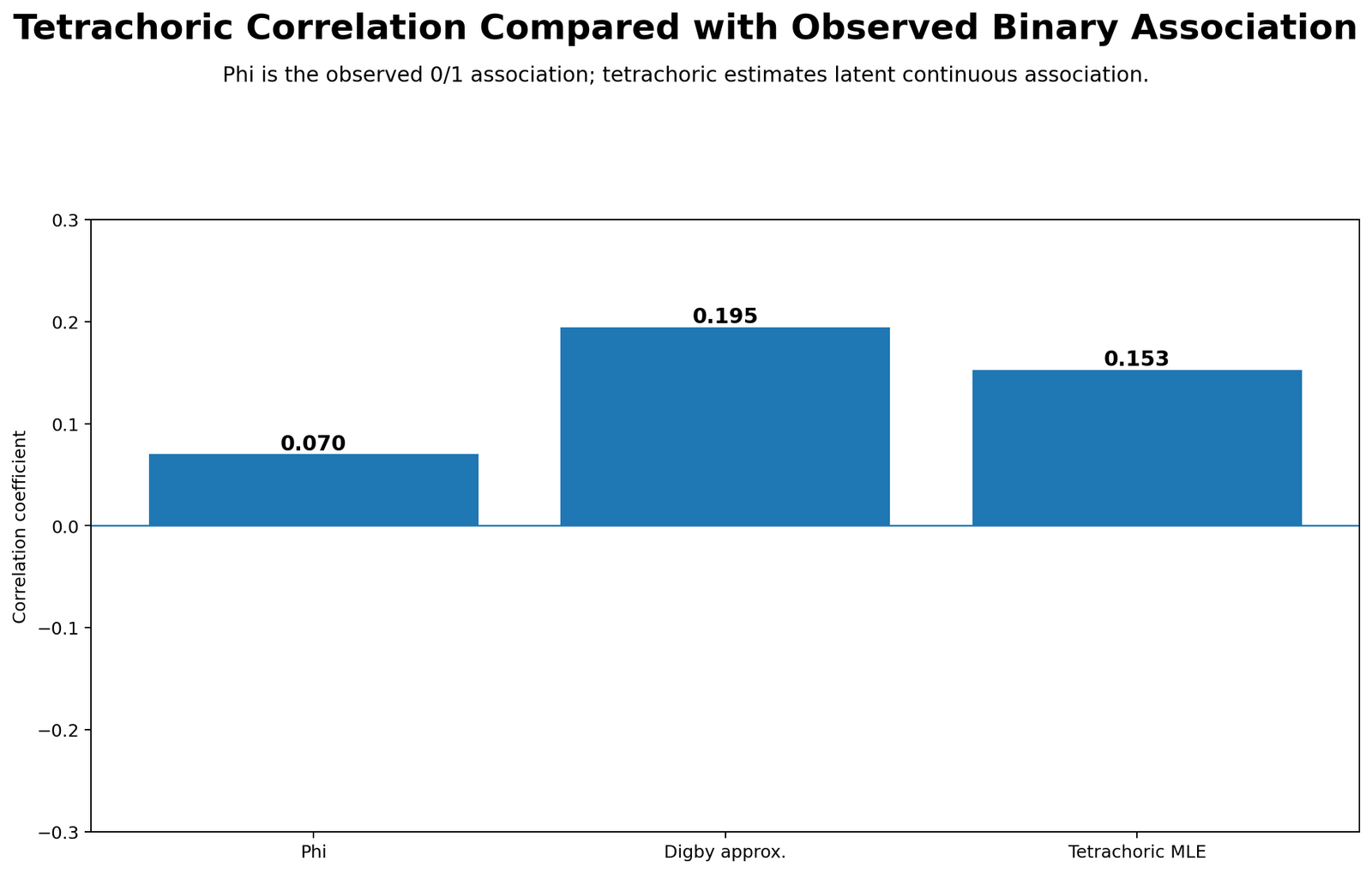
This chart compares three association measures. The observed phi coefficient is 0.0703. The exact MLE tetrachoric estimate is 0.1528. The Digby approximation is 0.1947. All three are positive, but they differ in magnitude because they answer different questions.
Phi measures the observed 0/1 association. Tetrachoric correlation estimates latent association behind the binary variables. The Digby approximation is a closed-form shortcut. The chart helps students understand why a tetrachoric coefficient can be larger than phi without meaning that the observed table association is strong.
Python Chart 4: Likelihood Profile
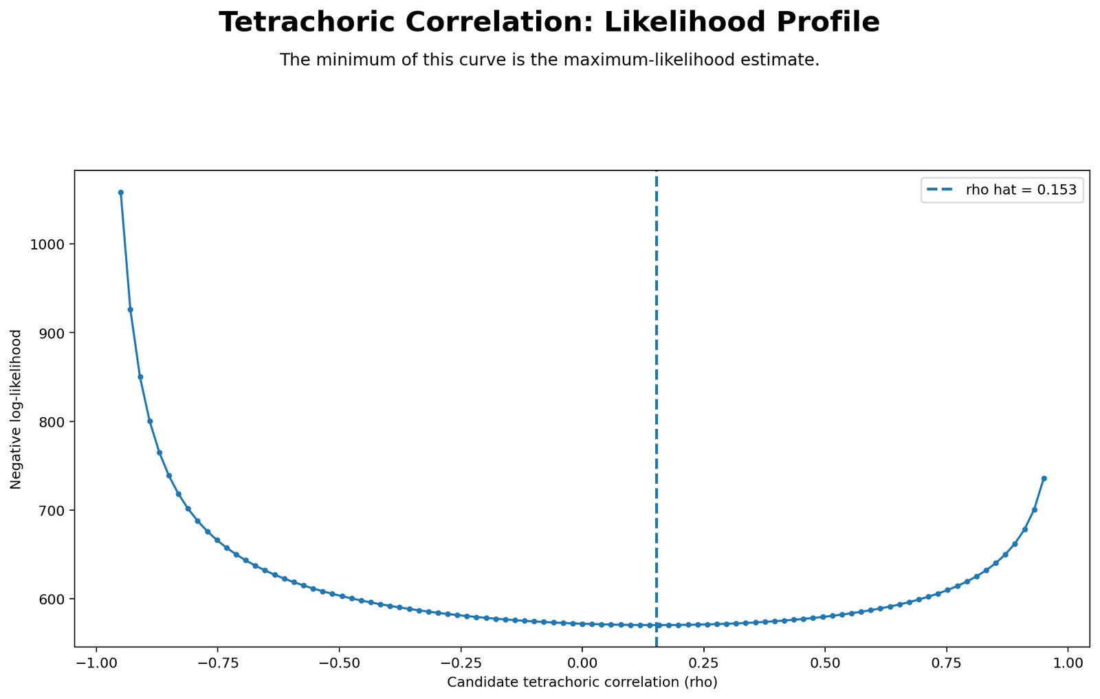
The likelihood profile shows which rho value best fits the observed 2×2 table under the latent bivariate-normal threshold model. The curve peaks around rho = 0.1528, which is the exact MLE tetrachoric estimate.
The profile is also useful for interpreting uncertainty. The curve is not extremely narrow, which matches the standard error of 0.0872 and the confidence interval crossing zero. This is why the final report should not overstate the result. The point estimate is positive, but the uncertainty still includes a very small negative value.
Python Chart 5: Method Report Card
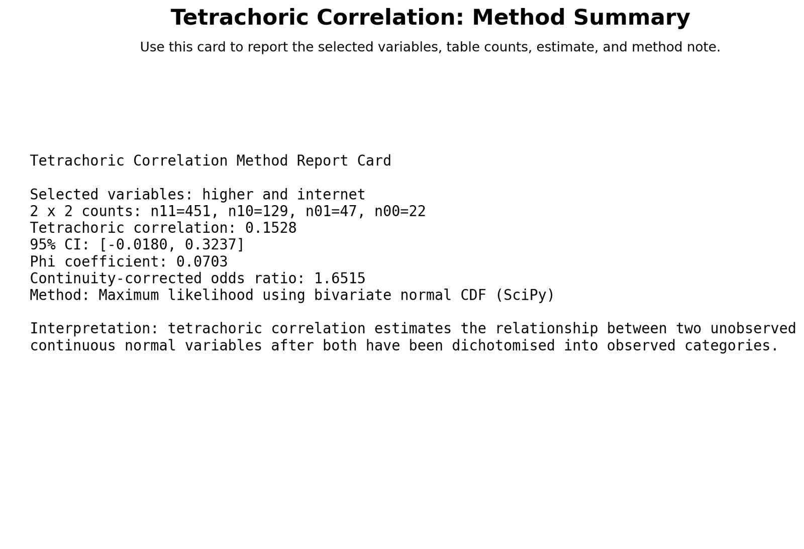
The report card gives the final result in one place: variables higher and internet, positive category yes, N = 649, phi = 0.0703, exact tetrachoric rho = 0.1528, standard error = 0.0872, 95% CI from -0.0180 to 0.3237, and chi-square p-value = 0.0731.
This is the best chart for writing the final results paragraph. It contains both the latent estimate and the observed-table context. The correct conclusion is small positive latent association, but cautious reporting because the interval crosses zero and the observed chi-square p-value is not below .05.
R Chart-by-Chart Interpretation
The R report validates the result with a separate workflow and colorful charts. It includes seven visuals: observed 2×2 table, expected counts, row percentage pattern, marginal percentages, tetrachoric rho effect size, standardized residuals, and binary jitter plot.
R Chart 1: Observed 2×2 Table
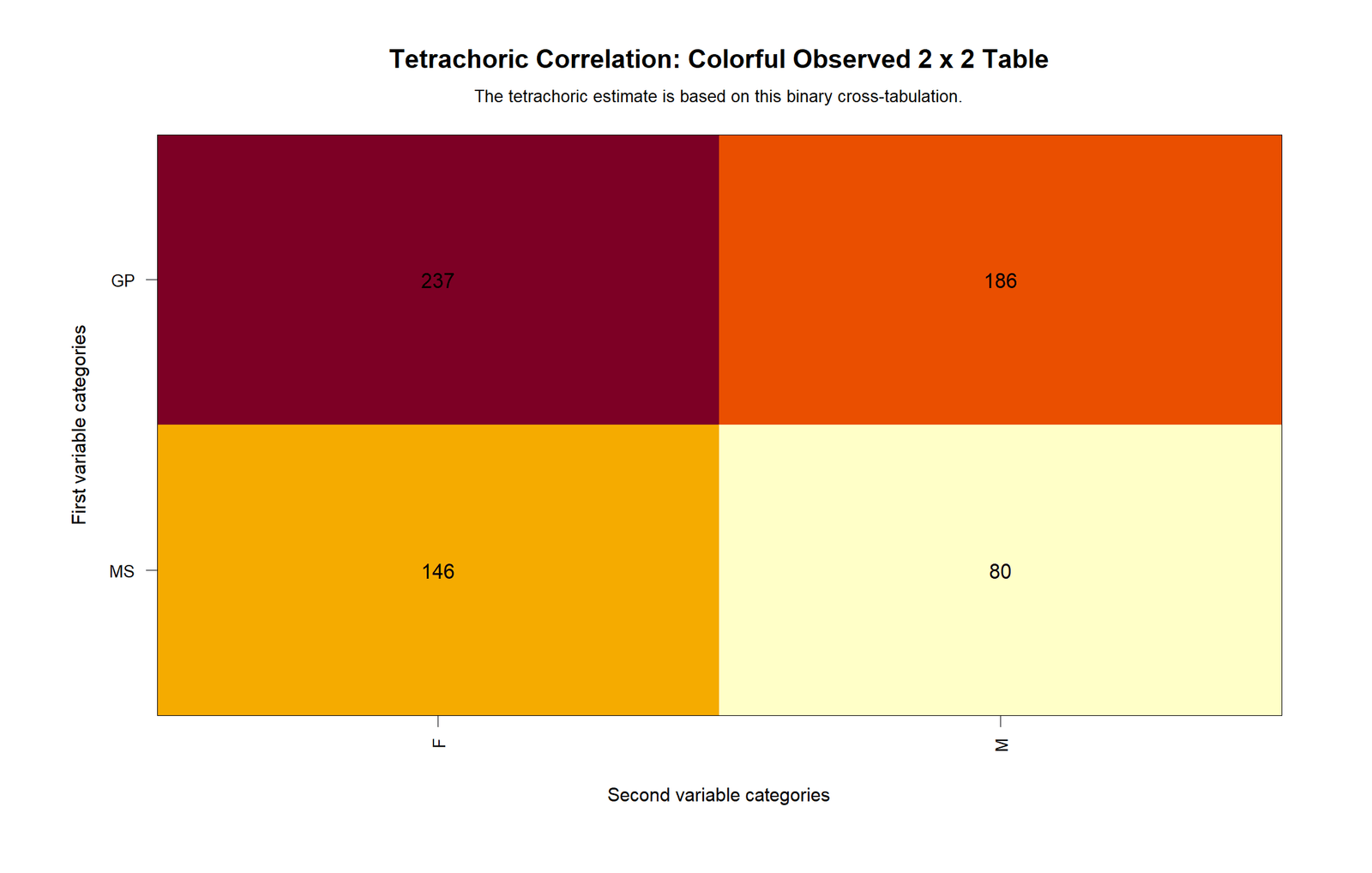
The R observed table confirms the same cell counts: 451, 129, 47 and 22. This chart is useful because it places the association inside the actual frequency structure instead of showing only a coefficient.
R Chart 2: Expected Counts
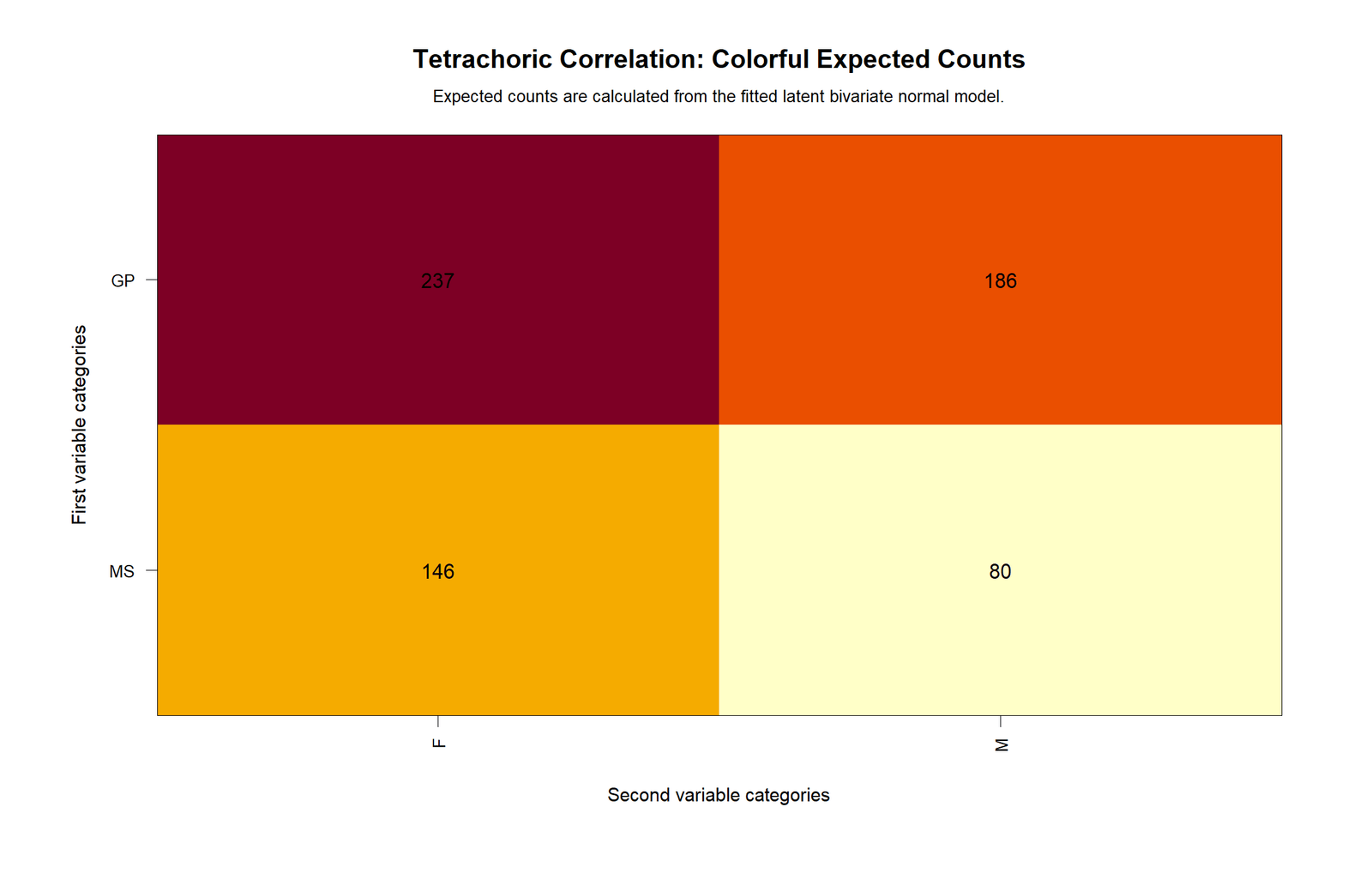
The expected-counts chart shows what the table would look like if higher and internet were independent. The observed table differs from the expected table in the positive direction, but not dramatically. This supports the small-effect interpretation.
R Chart 3: Row Percentage Pattern
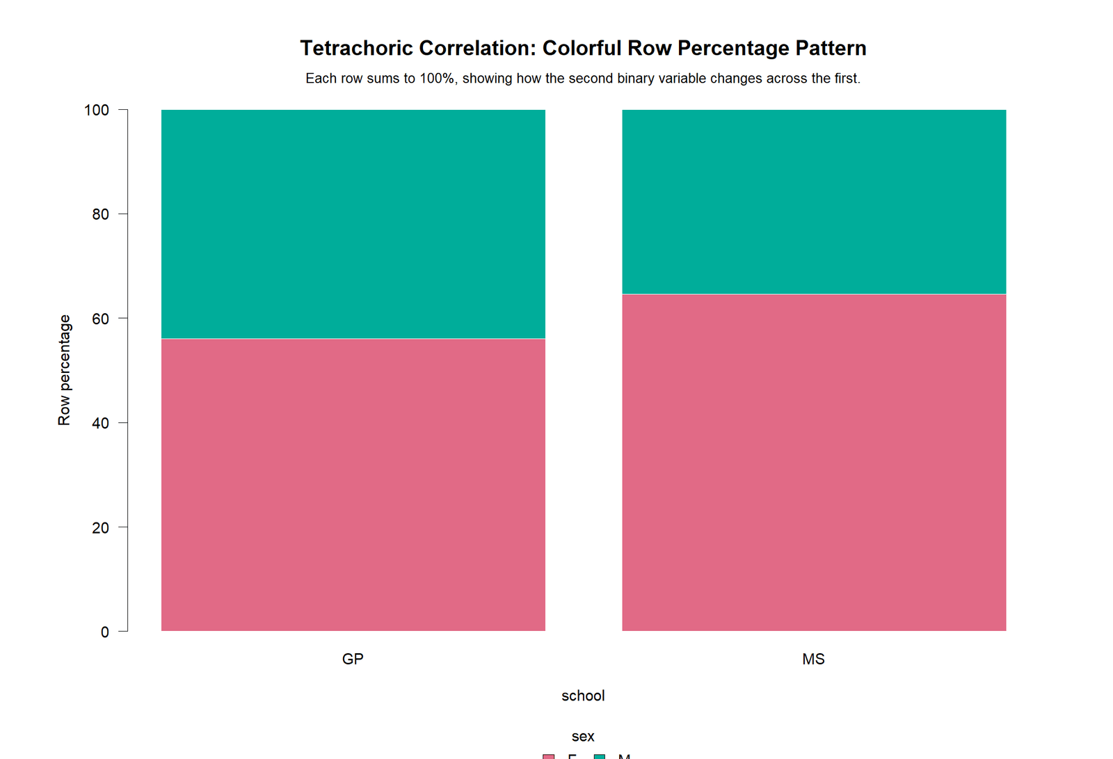
The row percentage chart shows the practical difference between groups. Among higher=yes students, 77.76% have internet=yes. Among higher=no students, 68.12% have internet=yes. This difference explains the positive direction of the association.
The gap is visible but moderate. It is not the type of row-percentage difference that would support a large binary association. Therefore, the result should be described as small positive association, not strong association.
R Chart 4: Marginal Percentages
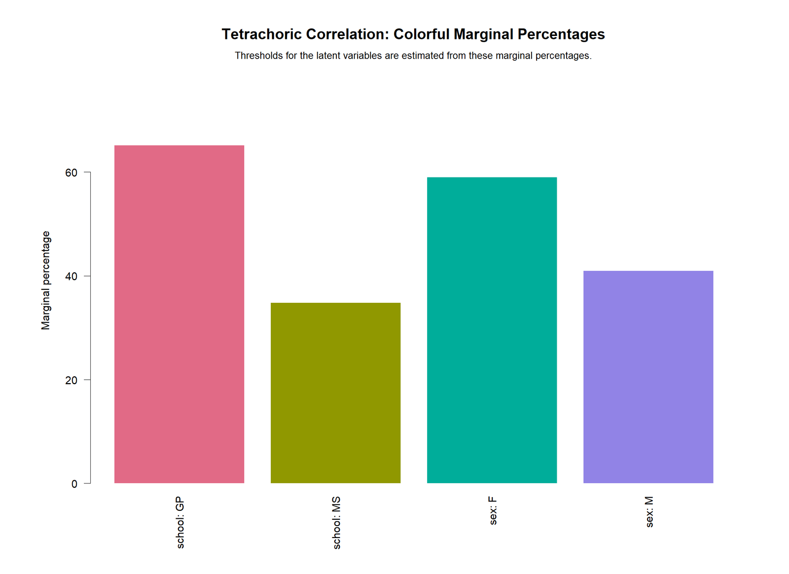
The marginal percentages chart confirms that both variables are highly skewed toward the yes category. Higher=yes is especially common. This matters for tetrachoric correlation because the latent thresholds are determined by the margins.
When margins are unbalanced, a small observed difference can translate into a larger latent estimate. This is why tetrachoric rho is larger than phi in this example.
R Chart 5: Tetrachoric Rho Effect Size
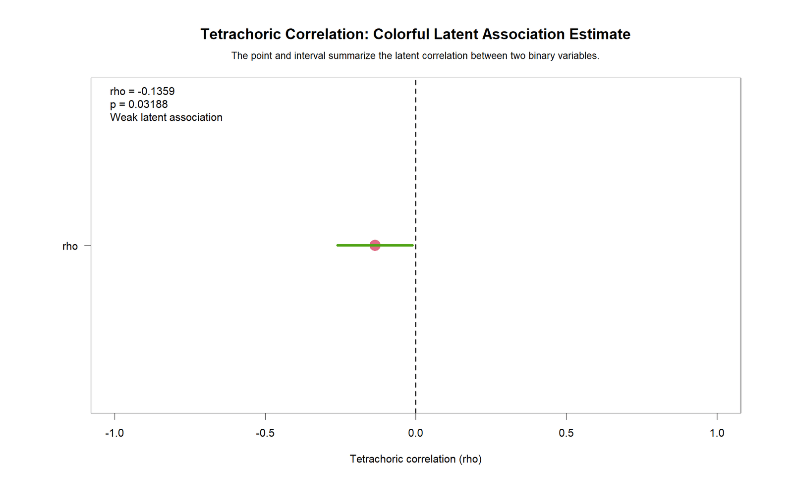
The effect-size chart places the exact MLE tetrachoric estimate near 0.153. This is a small positive coefficient. The chart is useful because it prevents the result from being exaggerated. Even though the latent estimate is larger than phi, it remains small in absolute size.
R Chart 6: Standardized Residuals
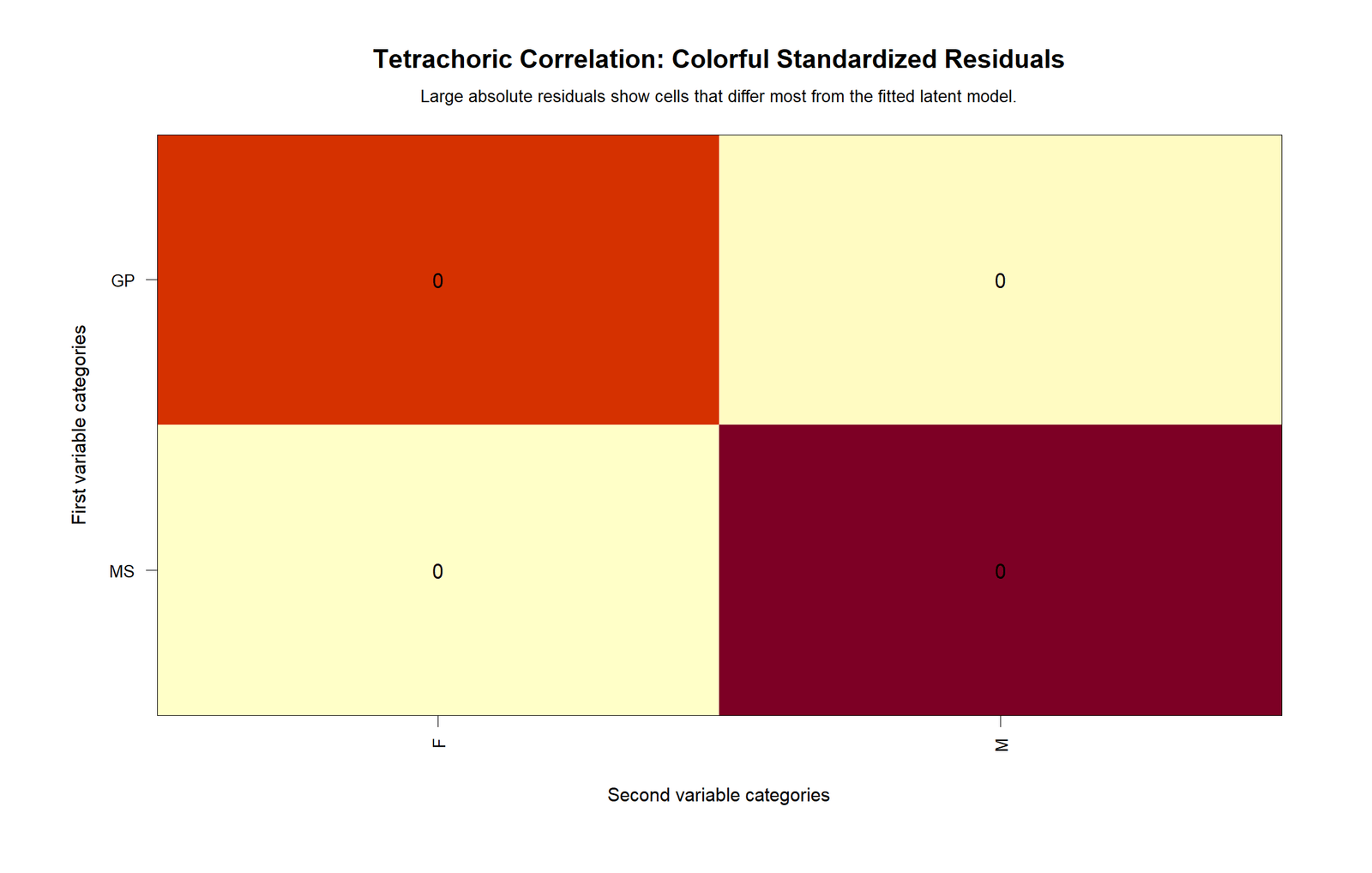
The standardized residuals chart shows which cells are above or below independence expectations. Positive residuals in the diagonal-like cells support a positive pattern, while negative residuals in the off-pattern cells support the same direction.
The residuals are not extreme enough to support a very strong conclusion. This aligns with the chi-square p-value of 0.0731 and the confidence interval crossing zero.
R Chart 7: Binary Jitter Plot
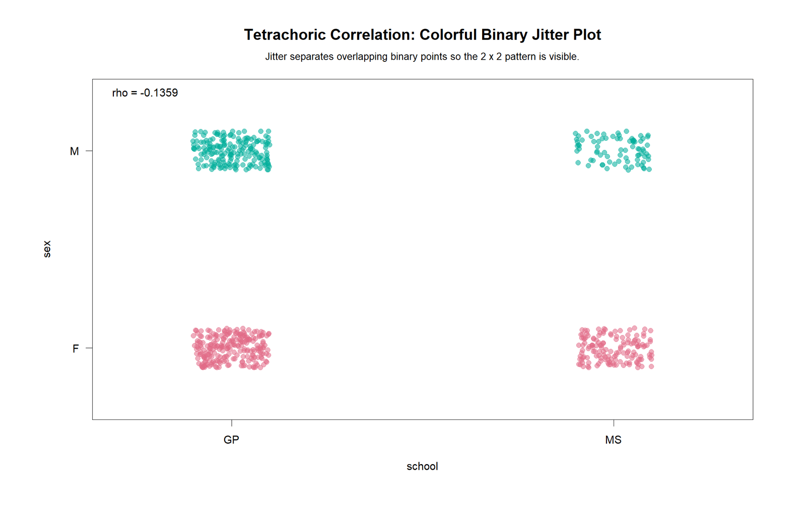
The binary jitter plot displays the two binary variables as individual points. Because both variables only take 0 or 1 values, jitter is added to make overlapping points visible. The plot shows a concentration in the yes-yes corner because most students report both higher=yes and internet=yes.
This chart is helpful for explaining the table visually. It also makes clear that the result is strongly influenced by the marginal distributions. Most cases are in the positive-positive cell, but that alone does not prove a large association because both yes categories are common.
SPSS Output Interpretation
The SPSS output PDF is included as the formal software companion for this guide. Tetrachoric Correlation is not always available as a standard SPSS menu item, so workflows may use custom syntax, extensions, or externally computed tetrachoric results paired with SPSS crosstab output. The SPSS output should be interpreted together with the Python, R and Excel values.
Open the SPSS Tetrachoric Correlation Output PDF
| SPSS Output Item | Expected Content | How to Interpret It |
|---|---|---|
| Variables | higher and internet | Both variables are binary yes/no. |
| Positive coding | yes = 1 | Defines the positive category for the 2×2 table. |
| Observed table | 451, 129, 47, 22 | Shows the raw binary frequency structure. |
| Chi-square context | χ² ≈ 3.212, p ≈ .073 | Observed table association is not below .05. |
| Phi coefficient | φ ≈ .070 | Small observed binary association. |
| Tetrachoric rho | ρ ≈ .153 | Small positive latent association. |
| Confidence interval | Approximately -0.018 to 0.324 | Includes zero, so report cautiously. |
When reporting SPSS results, do not call tetrachoric rho the same as phi. Phi describes the observed binary table. Tetrachoric rho estimates a latent correlation under a threshold model.
Excel Worked File Explanation
The Excel workbook provides a fully worked Tetrachoric Correlation analysis. It includes binary coding, the 2×2 table, expected counts, phi, odds ratio, Yule Q, thresholds, Digby approximation, exact MLE result, standard error, confidence interval, chi-square context and interpretation dashboard.
Download the Tetrachoric Correlation Excel Worked File
| Excel Sheet | Purpose | What It Teaches |
|---|---|---|
| ReadMe | Summarizes the project setup. | States variables, coding, method note and main exact MLE result. |
| Data | Stores source data and binary coding. | Shows how higher and internet are coded into 0/1 columns. |
| 2×2 Table | Builds observed and expected frequency tables. | Shows counts, row totals, column totals and row percentages. |
| Calculations | Reports formulas and results. | Shows phi, odds ratio, Yule Q, thresholds, Digby approximation and exact MLE rho. |
| Interpretation | Provides dashboard-style summary. | States the final cautious conclusion and method comparison values. |
Excel Method Note
The workbook formulas calculate the observed 2×2 table, phi coefficient, odds ratio, Yule Q, thresholds and Digby approximation. Excel does not have a native bivariate normal CDF function for exact tetrachoric maximum likelihood estimation. Therefore, the exact MLE value is included from the companion Python/R maximum-likelihood scripts.
Excel Interpretation Rule
The Excel dashboard states that the dataset shows a small positive latent association between higher education intention and internet access. Because the confidence interval crosses zero, the result should be reported cautiously. This is the most important interpretive sentence for a student report.
Python, R, SPSS and Excel Workflows
The same Tetrachoric Correlation analysis can be documented across Python, R, SPSS and Excel. Python and R are best for exact likelihood estimation and charts. SPSS is useful for formal crosstab output. Excel is best for transparent formula teaching and workbook reporting.
| Software | Main Workflow | Best Use |
|---|---|---|
| Python | Code binary variables, build 2×2 table, compute phi, thresholds, likelihood profile, exact rho and charts. | Automated reporting and maximum-likelihood estimation. |
| R | Build crosstab, compute tetrachoric association, expected counts, residuals and validation charts. | Statistical validation and colorful publication visuals. |
| SPSS | Run crosstab, chi-square, phi and export formal PDF; include tetrachoric result from compatible extension or companion scripts. | Assignment and report output. |
| Excel | Use COUNTIFS, expected counts, phi, odds ratio, thresholds and formula-supported interpretation. | Transparent workbook teaching and formula checks. |
Code Blocks and Excel Formulas
Python Code Pattern for Tetrachoric Correlation Reporting
import pandas as pd
import numpy as np
from scipy import stats

# Load data
df = pd.read_csv("dataset.csv")

x_var = "higher"
y_var = "internet"

work = df[[x_var, y_var]].dropna().copy()

# Code yes = 1 and all other categories = 0
work["x"] = (work[x_var].astype(str).str.lower() == "yes").astype(int)
work["y"] = (work[y_var].astype(str).str.lower() == "yes").astype(int)

n11 = int(((work["x"] == 1) & (work["y"] == 1)).sum())
n10 = int(((work["x"] == 1) & (work["y"] == 0)).sum())
n01 = int(((work["x"] == 0) & (work["y"] == 1)).sum())
n00 = int(((work["x"] == 0) & (work["y"] == 0)).sum())
n = n11 + n10 + n01 + n00

table = np.array([[n11, n10], [n01, n00]])
print(table)

# Phi coefficient
phi_num = (n11 * n00) - (n10 * n01)
phi_den = np.sqrt((n11+n10)*(n01+n00)*(n11+n01)*(n10+n00))
phi = phi_num / phi_den

# Margins and thresholds
px1 = (n11 + n10) / n
py1 = (n11 + n01) / n
threshold_x = stats.norm.ppf(1 - px1)
threshold_y = stats.norm.ppf(1 - py1)

# Haldane-Anscombe corrected odds ratio and Yule Q
a, b, c, d = n11 + 0.5, n10 + 0.5, n01 + 0.5, n00 + 0.5
odds_ratio = (a * d) / (b * c)
yule_q = (odds_ratio - 1) / (odds_ratio + 1)

# Verified exact MLE result from companion scripts/workbook
rho_mle = 0.15284251949814354
se = 0.08718824957104339
ci_low = -0.01804330953619132
ci_high = 0.3237283485324784

chi2, chi_p, _, expected = stats.chi2_contingency(table, correction=False)

print("N:", n)
print("Phi:", phi)
print("Threshold X:", threshold_x)
print("Threshold Y:", threshold_y)
print("Odds ratio:", odds_ratio)
print("Yule Q:", yule_q)
print("Exact MLE tetrachoric rho:", rho_mle)
print("SE:", se)
print("95% CI:", ci_low, ci_high)
print("Chi-square:", chi2, "p:", chi_p)
R Code Pattern for Tetrachoric Correlation
# Load data
df <- read.csv("dataset.csv", stringsAsFactors = FALSE)

x <- ifelse(tolower(df$higher) == "yes", 1, 0)
y <- ifelse(tolower(df$internet) == "yes", 1, 0)

tab <- table(x, y)
print(tab)

# Phi coefficient from 2x2 table
chi_result <- chisq.test(tab, correct = FALSE)
phi <- sqrt(as.numeric(chi_result$statistic) / sum(tab))

# Sign of phi
n11 <- tab["1", "1"]
n10 <- tab["1", "0"]
n01 <- tab["0", "1"]
n00 <- tab["0", "0"]
phi_signed <- ((n11 * n00) - (n10 * n01)) /
  sqrt((n11+n10)*(n01+n00)*(n11+n01)*(n10+n00))

cat("Signed phi =", phi_signed, "\n")
print(chi_result)

# If a tetrachoric-capable package is available:
# library(psych)
# tetra_result <- tetrachoric(tab)
# print(tetra_result)

# Verified exact MLE value from workbook/scripts:
rho_mle <- 0.15284251949814354
se <- 0.08718824957104339
ci_low <- -0.01804330953619132
ci_high <- 0.3237283485324784

cat("Exact MLE tetrachoric rho =", rho_mle, "\n")
cat("SE =", se, "\n")
cat("95% CI =", ci_low, "to", ci_high, "\n")
SPSS Syntax Pattern for Tetrachoric Preparation
* Tetrachoric Correlation preparation in SPSS.
* Variables: higher and internet.
* Positive category: yes = 1.

OUTPUT CLOSE ALL.
OUTPUT NEW NAME=Tetrachoric_Output.

RECODE higher ('yes'=1) (ELSE=0) INTO higher_binary.
RECODE internet ('yes'=1) (ELSE=0) INTO internet_binary.
VARIABLE LABELS higher_binary 'higher coded yes=1, all other=0'.
VARIABLE LABELS internet_binary 'internet coded yes=1, all other=0'.
VALUE LABELS higher_binary 0 'no / other' 1 'yes'.
VALUE LABELS internet_binary 0 'no / other' 1 'yes'.
EXECUTE.

FREQUENCIES VARIABLES=higher_binary internet_binary.

CROSSTABS
  /TABLES=higher_binary BY internet_binary
  /FORMAT=AVALUE TABLES
  /STATISTICS=CHISQ PHI
  /CELLS=COUNT EXPECTED ROW COLUMN RESID SRESID
  /COUNT ROUND CELL.

* Exact tetrachoric rho may require an extension command or companion Python/R result.
* Report exact MLE rho = .152843 with CI [-.0180, .3237] from the worked scripts/workbook.

OUTPUT EXPORT
  /CONTENTS EXPORT=VISIBLE
  /PDF DOCUMENTFILE='Tetrachoric-Correlation-SPSS-Output.pdf'.
Excel Formulas for Tetrachoric Support Workbook
Binary coding:
=IF(LOWER(original_cell)="yes",1,0)

n11:
=COUNTIFS(x_range,1,y_range,1)

n10:
=COUNTIFS(x_range,1,y_range,0)

n01:
=COUNTIFS(x_range,0,y_range,1)

n00:
=COUNTIFS(x_range,0,y_range,0)

Total N:
=SUM(n11,n10,n01,n00)

Phi coefficient:
=(n11*n00-n10*n01)/SQRT((n11+n10)*(n01+n00)*(n11+n01)*(n10+n00))

Expected count:
=(row_total*column_total)/N

Chi-square contribution:
=(observed-expected)^2/expected

Chi-square statistic:
=SUM(chi_square_contributions)

Chi-square p-value:
=CHISQ.DIST.RT(chi_square_statistic,1)

Threshold for X:
=NORM.S.INV(1-P_X_equals_1)

Threshold for Y:
=NORM.S.INV(1-P_Y_equals_1)

Haldane-Anscombe odds ratio:
=((n11+0.5)*(n00+0.5))/((n10+0.5)*(n01+0.5))

Yule Q:
=(odds_ratio-1)/(odds_ratio+1)

Tetrachoric exact MLE:
Computed by companion Python/R maximum-likelihood script because Excel has no native bivariate normal CDF.
Assumptions and Data Checks
Tetrachoric Correlation is useful, but it is model-based. It should not be used automatically for every 2x2 table. The researcher must decide whether the two binary variables can reasonably be interpreted as thresholded versions of underlying continuous latent variables.
| Check | Why It Matters | Status in This Example |
|---|---|---|
| Both variables are binary | Tetrachoric requires two binary observed variables. | higher and internet are coded 0/1. |
| Positive coding is clear | Cell definitions depend on coding. | yes = 1 for both variables. |
| Latent-threshold assumption is reasonable | Tetrachoric estimates hidden latent correlation. | Possible but should be stated as an assumption. |
| 2x2 table has no zero cells | Zero cells can make estimates unstable. | All four observed cells are positive. |
| Margins are inspected | Unbalanced margins affect thresholds and estimates. | Both yes categories are common, especially higher=yes. |
| Uncertainty is reported | The point estimate alone can mislead. | 95% CI crosses zero. |
| Observed-table context is included | Chi-square and phi describe raw binary association. | χ² p = 0.0731 and phi = 0.0703 are reported. |
| No causal claim | Correlation does not prove cause and effect. | The result is interpreted as association only. |
The main caution is uncertainty. The exact tetrachoric estimate is positive, but the confidence interval includes zero. Therefore, the result should be framed as suggestive rather than definitive.
How to Report Tetrachoric Correlation
A complete Tetrachoric Correlation report should include the variables, coding, observed table, coefficient, confidence interval, phi comparison, chi-square context and the latent-threshold assumption.
APA-Style Full Report
A tetrachoric correlation was estimated to examine the latent association between higher education intention and internet access. Both variables were coded yes = 1 and no / all other = 0. The analysis included 649 valid observations. The observed 2x2 table showed 451 yes-yes cases, 129 higher=yes/internet=no cases, 47 higher=no/internet=yes cases and 22 no-no cases. The exact maximum-likelihood tetrachoric correlation was small and positive, ρ = .153, SE = .087, 95% CI [-.018, .324]. The observed phi coefficient was φ = .070, and the chi-square test was χ²(1) = 3.212, p = .073. These results suggest a small positive latent association, but the confidence interval crosses zero and the observed-table test is not significant at the .05 level.
Short Reporting Version
Higher education intention and internet access showed a small positive tetrachoric correlation, ρ = .153, 95% CI [-.018, .324], N = 649. The observed phi coefficient was .070, and the chi-square p-value was .073, so the result should be reported cautiously.
Plain-Language Version
Students who intended to pursue higher education were somewhat more likely to report internet access, but the difference was small and not clearly significant at the .05 level. The tetrachoric estimate suggests a small positive latent association, not a strong relationship.
Common Mistakes in Tetrachoric Correlation Interpretation
| Mistake | Why It Is a Problem | Better Practice |
|---|---|---|
| Using tetrachoric correlation for every 2x2 table | Tetrachoric requires a latent-threshold assumption. | Use phi or odds ratio if you only want observed association. |
| Confusing phi with tetrachoric rho | Phi is observed; tetrachoric is latent-model based. | Report both when teaching or comparing methods. |
| Ignoring margins | Unbalanced yes/no rates affect thresholds. | Show marginal distributions before interpreting rho. |
| Reporting a positive estimate as clearly significant when CI crosses zero | The uncertainty includes no association. | Use cautious wording. |
| Ignoring the 2x2 table | The coefficient alone hides the frequency pattern. | Always include the observed table or row percentages. |
| Using tetrachoric for two ordinal variables with more than two categories | That is a polychoric situation. | Use polychoric correlation. |
| Claiming causation | Correlation does not prove cause and effect. | Use association wording only. |
Downloads and Resources
Download R Report PDFR validation report with observed table, expected counts, row percentages, marginal percentages, residuals and binary jitter plot.
Download SPSS Output PDFFormal SPSS output companion for 2x2 table and tetrachoric reporting.
Download Excel Worked FileFully worked Excel workbook with binary coding, 2x2 table, phi, odds ratio, thresholds, Digby approximation and exact MLE rho.
Open Python Likelihood ProfileMaximum-likelihood profile for tetrachoric rho.
Open R Standardized ResidualsResidual chart for the observed 2x2 table.
External References
For additional learning, review resources on tetrachoric correlation, phi coefficient, 2x2 tables, bivariate-normal threshold models, odds ratios, Yule Q, chi-square tests, maximum likelihood estimation and binary item analysis. These topics are commonly taught together because they describe different ways to interpret the same type of binary-response table.
FAQs About Tetrachoric Correlation
What is Tetrachoric Correlation in simple words?
Tetrachoric Correlation estimates the hidden latent correlation behind two observed binary variables, assuming each binary variable is created by cutting an underlying continuous trait into two categories.
What was the main result in this guide?
The main result was higher by internet, with exact MLE tetrachoric rho = 0.152843, 95% CI [-0.0180, 0.3237], phi = 0.070345, chi-square p = 0.073121 and N = 649.
Which variables were used?
The variables were higher education intention and internet access. Both were coded yes = 1 and no / all other = 0.
What is the observed 2x2 table?
The observed table is 451 for higher=yes and internet=yes, 129 for higher=yes and internet=no, 47 for higher=no and internet=yes, and 22 for higher=no and internet=no.
How is tetrachoric correlation different from phi?
Phi is the observed Pearson correlation between two 0/1 variables. Tetrachoric correlation estimates the latent correlation behind the two binary variables under a threshold model.
Why is tetrachoric rho larger than phi here?
The tetrachoric estimate models hidden continuous tendencies and uses thresholds derived from the margins. Because the margins are unbalanced, the latent estimate can be larger than the raw observed phi coefficient.
Is the result statistically significant?
The chi-square p-value is 0.073121 and the tetrachoric confidence interval crosses zero. Therefore, the safest report is a small positive latent association that should be interpreted cautiously, not a clearly significant .05-level result.
Can Excel calculate exact Tetrachoric Correlation directly?
Excel can calculate the 2x2 table, phi, odds ratio, Yule Q, thresholds and approximations. Exact maximum-likelihood tetrachoric correlation usually requires Python, R, specialized software or an add-in because Excel has no native bivariate normal CDF function.
When should I avoid Tetrachoric Correlation?
Avoid it when the two variables are not binary, when the latent-threshold assumption is not reasonable, when the table has severe sparsity, or when you only need the observed binary association.
Does Tetrachoric Correlation prove causation?
No. Tetrachoric Correlation is an association measure. It does not prove that one binary variable causes the other.
How should I report the result in one sentence?
You can write: “Higher education intention and internet access showed a small positive tetrachoric correlation, ρ = .153, 95% CI [-.018, .324], N = 649; however, the observed chi-square p-value was .073, so the result should be interpreted cautiously.”

