
Normality Test, Goodness-of-Fit, Tail Sensitivity, Empirical CDF and SPSS Output
Anderson Darling Test: Formula, Interpretation, SPSS, Python, R and Excel Guide
Anderson Darling Test is a goodness-of-fit and normality test that compares the empirical distribution of a sample with a specified theoretical distribution. It is especially useful because it gives extra weight to the tails of the distribution. That makes the Anderson Darling Test very valuable when you need to detect non-normality caused by heavy tails, light tails, outliers, skewness, or tail mismatch. In this complete Salar Cafe guide, you will learn the Anderson Darling Test with formula, null and alternative hypotheses, verified SPSS output interpretation, Python charts, R validation charts, Excel workflow, APA reporting, common mistakes, internal links, and downloadable resources.
Google AdSense top placement reserved here
Quick Answer: Anderson Darling Test Result
The Anderson Darling Test checks whether a sample follows a specified theoretical distribution, most commonly the normal distribution. The null hypothesis says the data follow the specified distribution. The alternative hypothesis says the data do not follow the specified distribution. The test statistic is usually written as A². A larger A² statistic means a stronger departure from the reference distribution. The test is particularly sensitive to departures in the lower and upper tails.
In a normality-testing workflow, the Anderson Darling Test should be interpreted with the distribution fit chart, normal Q-Q plot, empirical CDF versus fitted normal CDF chart, tail-weighted contribution chart, AD statistic across variables chart, and group AD statistic comparison chart. These visuals show whether the problem is a general shape mismatch, tail behavior, variable-specific non-normality, or group-specific distribution difference.
Final interpretation: The Anderson Darling Test is best reported as a tail-sensitive normality or distribution-fit test. If the p-value is below .05, reject the null hypothesis and conclude that the data differ significantly from the selected distribution. If the p-value is not below .05, the test does not provide sufficient evidence against the distribution. Always interpret the result with visual checks because the Anderson Darling Test often detects tail problems that a simple histogram may hide.
Important: The Anderson Darling Test is not the same as the Kolmogorov-Smirnov Test. The KS test focuses on the largest CDF gap, while the Anderson Darling Test weights the full CDF difference and gives more importance to the tails. For normality work, compare it with the Lilliefors Test, Cramer-von Mises Test, and D’Agostino-Pearson Test.
Table of Contents
- What Is the Anderson Darling Test?
- Why the Anderson Darling Test Matters
- Anderson Darling Test Formula
- Null and Alternative Hypotheses
- Assumptions and Decision Logic
- Dataset and Variables Used
- Verified SPSS Output Interpretation
- Python Chart-by-Chart Interpretation
- R Chart-by-Chart Validation
- SPSS, Python, R and Excel Workflows
- SPSS, Python, R and Excel Code
- APA Reporting Wording
- Common Mistakes
- When to Use the Anderson Darling Test
- Downloads and Resources
- Related Internal Guides
- FAQs
What Is the Anderson Darling Test?
The Anderson Darling Test is a statistical goodness-of-fit test used to determine whether sample data follow a specified probability distribution. In applied research, it is most often used as a normality test. It compares the empirical cumulative distribution function of the sample with the theoretical cumulative distribution function of the selected distribution.
The special feature of the Anderson Darling Test is its tail sensitivity. While some normality tests focus mostly on the middle of the distribution or the single largest gap, the Anderson Darling Test gives more weight to differences in the lower and upper tails. This makes it especially useful when the main issue is outliers, heavy tails, light tails, skewed tail behavior, or extreme-score mismatch.
Simple definition: The Anderson Darling Test checks whether the observed distribution follows a selected theoretical distribution, with extra attention to the tails.
For a full normality analysis, use the Anderson Darling Test with the Q-Q Plot Normality Check, Q-Q Plot Normality Check 2, P-P Plot Normality Check, Histogram Interpretation, and Box Plot Interpretation. These plots show the shape behind the formal test statistic.
Why the Anderson Darling Test Matters
The Anderson Darling Test matters because many statistical methods assume that variables, residuals, or errors are approximately normally distributed. This assumption can affect t tests, ANOVA, regression, confidence intervals and many parametric procedures. However, not all non-normality looks the same. Sometimes the center of the distribution looks acceptable, but the tails are too heavy or too light. The Anderson Darling Test is useful because it is designed to detect these tail problems.
For example, a student performance variable may look roughly bell-shaped in the center but show unusual extreme scores at the low end or high end. A histogram might not make that tail problem obvious, but the Anderson Darling Test and tail-weighted contribution plot can show it clearly. This is why the test is often stronger than relying on one visual alone.
| Diagnostic Need | Why Anderson Darling Helps | Related Guide |
|---|---|---|
| Normality testing | Tests whether the sample follows a normal distribution. | Lilliefors Test |
| Tail sensitivity | Gives extra weight to lower and upper tail deviations. | Q-Q Plot Normality Check |
| Distribution-fit comparison | Compares empirical CDF with fitted theoretical CDF. | Cramer-von Mises Test |
| Outlier and extreme-value sensitivity | Tail weighting makes extreme-score mismatch easier to detect. | Box Plot Interpretation |
| Assumption reporting | Provides formal evidence for normality decisions. | Descriptive Statistics |
Because the Anderson Darling Test is sensitive, it should be interpreted with sample size and practical shape. In large samples, small deviations may become statistically significant. In small samples, visual diagnostics and additional tests such as the Ryan-Joiner Test can help confirm the conclusion.
Anderson Darling Test Formula
The Anderson Darling Test statistic is usually written as A². It compares sorted sample values with the cumulative probabilities expected under the reference distribution.
Where:
| Symbol | Meaning | Interpretation |
|---|---|---|
| A² | Anderson Darling statistic | Larger values indicate stronger departure from the reference distribution. |
| n | Sample size | Number of valid observations used in the test. |
| xi | Sorted sample value | Observed value arranged from smallest to largest. |
| F(x) | Theoretical cumulative distribution function | Expected cumulative probability under the selected distribution. |
| ln | Natural logarithm | Creates tail weighting through log probabilities near 0 and 1. |
Why the Formula Is Tail Sensitive
The Anderson Darling formula uses logarithmic terms involving F(x) and 1 − F(x). These terms become very important in the lower and upper tails, where cumulative probabilities are close to 0 or 1. That is why the Anderson Darling Test detects tail departures more strongly than many simpler distribution-fit checks.
Formula caution: When a normal distribution is fitted using sample mean and sample standard deviation, some software uses adjusted Anderson Darling statistics or p-value approximations. Always report the statistic and p-value or critical-value decision according to the software output used.
Null and Alternative Hypotheses for the Anderson Darling Test
The Anderson Darling Test is a formal hypothesis test. For normality testing, the null hypothesis states that the sample comes from a normal distribution. The alternative states that the sample does not come from a normal distribution.
| Hypothesis | Statement | Meaning for Reporting |
|---|---|---|
| Null hypothesis | H0: The data follow the selected distribution. | For normality testing, the data are consistent with a normal distribution. |
| Alternative hypothesis | H1: The data do not follow the selected distribution. | The distribution-fit or normality assumption is not supported. |
| Decision rule using p-value | Reject H0 if p < .05. | A significant result indicates departure from the reference distribution. |
| Decision rule using critical values | Reject H0 if A² exceeds the critical value. | The statistic is too large for the chosen significance level. |
Decision wording: If the Anderson Darling p-value is below .05, report that the distribution differs significantly from normal. If the p-value is not below .05, report that the test did not provide sufficient evidence to reject normality.
If the normality decision affects a parametric analysis, connect this result with the Central Limit Theorem, Confidence Interval interpretation, Effect Size, and the specific test being used, such as a One-Tailed T Test, One Sample Z Test, or One Proportion Z Test.
Assumptions and Decision Logic
The Anderson Darling Test is used to assess distribution fit, but its interpretation still depends on proper data handling. The variable should be numeric, observations should be independent, and the chosen reference distribution should make sense for the variable. For normality testing, use a variable or residual series where normality is actually relevant.
| Requirement | Why It Matters | Recommended Action |
|---|---|---|
| Numeric data | The test compares continuous distribution patterns. | Use continuous or approximately continuous variables. |
| Independent observations | Dependency can distort distribution testing. | Check study design before interpreting p-values. |
| Correct reference distribution | Testing normality only makes sense when normality is relevant. | Choose normal, exponential, logistic or another distribution based on research purpose and software support. |
| Tail review | Anderson Darling is tail-sensitive. | Use Q-Q plot, tail contribution plot and box plot. |
| Sample-size awareness | Large samples may detect small departures. | Interpret p-value with practical visual shape. |
For a complete assumption-testing workflow, do not confuse normality with variance assumptions. Use tests such as the Levene Test, Brown-Forsythe Test, Cochran C Test, and Goldfeld-Quandt Test when the research question is about equal variance or heteroscedasticity rather than normality.
Interpretation caution: The Anderson Darling Test is sensitive in the tails. A significant result may be driven by a few extreme observations, so always check the normal Q-Q plot, box plot, and tail-weighted contribution chart before choosing a transformation or nonparametric method.
Dataset and Variables Used
The worked Anderson Darling Test example uses student performance variables. The main normality workflow can be applied to a numeric variable such as G3 final grade, while the cross-variable chart compares Anderson Darling statistics across multiple numeric variables. A group comparison chart also shows whether distribution-fit concerns differ across categories.
| Dataset Element | Role in Anderson Darling Test | Why It Matters |
|---|---|---|
| Main numeric variable | Primary normality-test variable | Used for distribution fit, Q-Q plot and ECDF comparison. |
| Empirical CDF | Observed cumulative distribution | Compared with the fitted theoretical distribution. |
| Fitted normal CDF | Reference distribution | Shows expected cumulative probabilities under normality. |
| Tail contributions | Lower and upper tail diagnostics | Explain where Anderson Darling statistic receives high weight. |
| Multiple numeric variables | AD statistic comparison | Shows which variables depart more strongly from normality. |
| Group variable | Subgroup distribution comparison | Shows whether normality problems differ across groups. |
Before running the Anderson Darling Test, review each variable with Descriptive Statistics, Frequency Distribution, Histogram Interpretation, Five Number Summary, Coefficient of Variation, and Box Plot Interpretation.
Google AdSense middle placement reserved here
Verified SPSS Output Interpretation for the Anderson Darling Test
The SPSS output PDF supports the Anderson Darling Test normality workflow for this post. In SPSS-style reporting, the result should be interpreted with the test statistic, p-value or critical-value decision, histogram, Q-Q plot, empirical CDF interpretation, and tail-focused explanation. Because SPSS workflows can vary by extension, syntax, custom calculation or integrated output, the key reporting point is the same: state whether the observed distribution differs from the fitted normal distribution.
How to Read the SPSS Output
| SPSS Output Item | What It Means | How to Interpret |
|---|---|---|
| Anderson Darling statistic | A² or adjusted A² value | Larger values indicate stronger departure from the selected distribution. |
| p-value or significance level | Formal decision measure | If p < .05, reject the normality assumption. |
| Critical value comparison | A² compared with critical threshold | If A² exceeds the critical value, reject the distribution fit. |
| Histogram or distribution plot | Observed shape versus normal reference | Explains whether the center, tails or outliers cause departure. |
| Q-Q plot | Observed quantiles versus expected normal quantiles | Shows tail deviations and nonlinear departures. |
| Descriptive statistics | Mean, standard deviation, skewness, kurtosis | Provides context for distribution-shape interpretation. |
SPSS Decision Logic
If the SPSS-supported Anderson Darling p-value is below .05, report that the test found a significant departure from normality. If the p-value is above .05, report that the test did not provide sufficient evidence against normality. If the output uses critical values instead of a p-value, compare the statistic with the critical value at the chosen significance level.
SPSS conclusion template: The Anderson Darling Test was used to evaluate whether the variable followed a normal distribution. The statistic and significance decision were interpreted together with the distribution fit chart, normal Q-Q plot and empirical CDF evidence. The final decision was based on whether the observed distribution showed a statistically meaningful departure from the fitted normal distribution.
SPSS reporting caution: Do not treat the Anderson Darling Test as only a center-of-distribution test. Its strength is tail sensitivity. In SPSS interpretation, mention whether the plots suggest tail mismatch, outliers or broader non-normality.
Python Chart-by-Chart Interpretation
The Python charts provide a full Anderson Darling Test visual workflow. They show distribution fit, normal Q-Q plot, empirical CDF versus fitted normal CDF, tail-weighted contributions, AD statistic across variables and group AD statistic comparison.
Python Chart 1: Distribution Fit for Anderson Darling Test
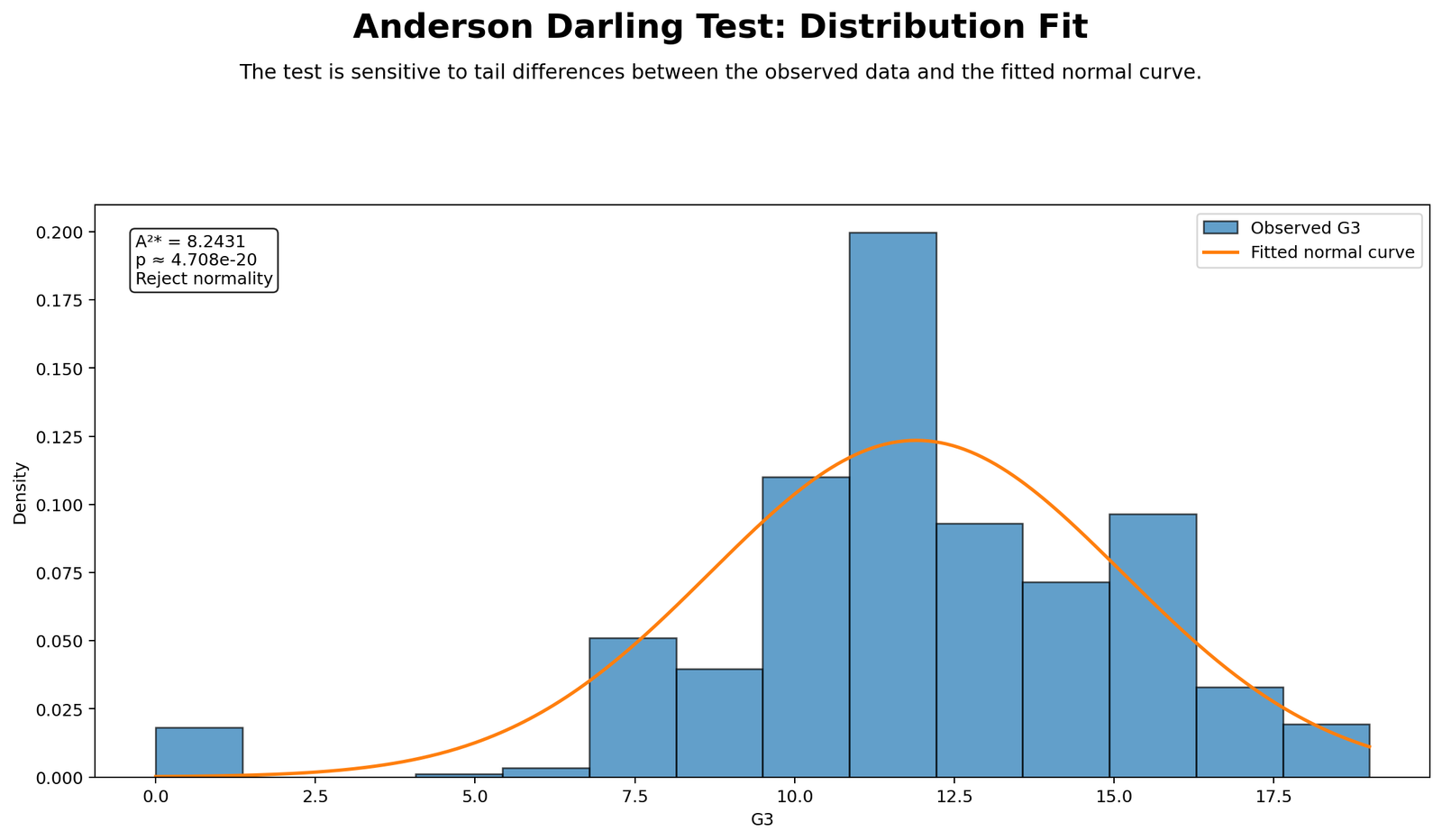
This chart gives the first visual explanation of the Anderson Darling Test. It compares the sample distribution with a fitted normal curve. If the bars or density shape align closely with the fitted curve, normality is more plausible. If the chart shows skewness, heavy tails, outliers, multiple peaks or strong tail mismatch, the Anderson Darling statistic may become larger.
The distribution fit chart is especially useful because the Anderson Darling Test is sensitive to tail behavior. A distribution can look acceptable near the center but still fail because of lower-tail or upper-tail deviations. This chart provides the practical shape context before reviewing the more technical tail-weighted contribution chart.
Decision/reporting conclusion: Use this Python distribution fit chart as the first visual support for the Anderson Darling decision. If the shape visibly departs from the fitted normal curve, report that the chart supports possible non-normality.
Python Chart 2: Normal Q-Q Plot
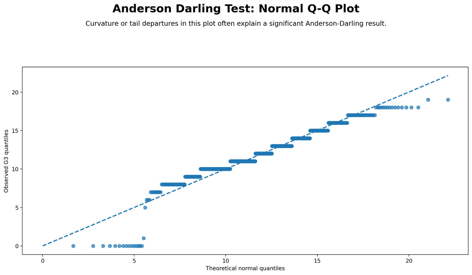
The Q-Q plot is one of the best visual companions to the Anderson Darling Test. If the points follow the diagonal line, the distribution is close to normal. If the points curve away from the line, especially at the lower or upper ends, the distribution has tail departures. Since Anderson Darling is tail-sensitive, Q-Q plot tail deviations are highly relevant.
A downward or upward curve can suggest skewness. Points far from the diagonal at the ends can suggest heavy tails, light tails or outliers. This chart helps explain why the Anderson Darling statistic may be large even when the histogram looks acceptable.
Decision/reporting conclusion: Use this Q-Q plot to explain whether the Anderson Darling result is driven by center mismatch, lower-tail deviation, upper-tail deviation or extreme observations.
Python Chart 3: Empirical CDF vs Fitted Normal CDF
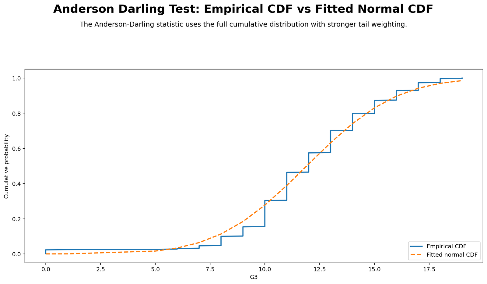
This chart shows the distribution comparison at the cumulative probability level. The empirical CDF shows the observed cumulative pattern of the sample. The fitted normal CDF shows the expected cumulative pattern if the data were normally distributed. The Anderson Darling Test measures weighted differences between these cumulative functions.
Unlike a simple maximum-gap view, Anderson Darling considers differences across the distribution and weights tail discrepancies more heavily. Therefore, this chart should be read carefully at the lower and upper ends as well as the middle.
Decision/reporting conclusion: Use this ECDF chart to explain where the observed cumulative distribution differs from the fitted normal distribution. Tail separation supports the logic of an Anderson Darling warning.
Python Chart 4: Tail-Weighted Contributions
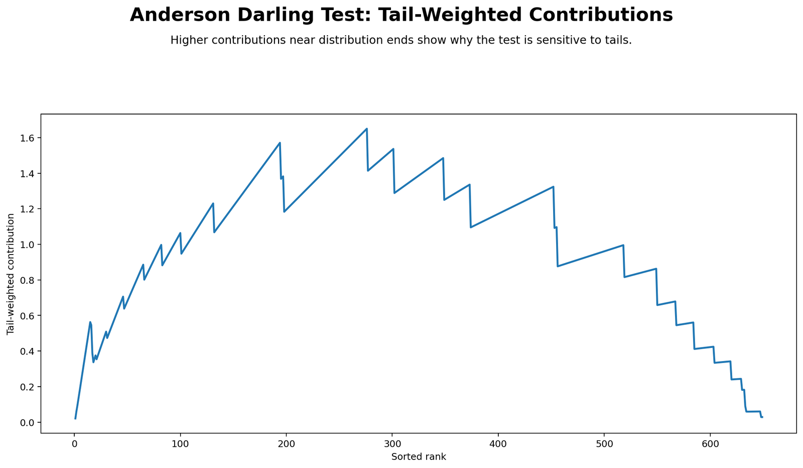
This is the most distinctive Anderson Darling chart. It shows which parts of the distribution contribute most strongly to the Anderson Darling statistic. Because the test weights tail deviations heavily, the lower and upper tails can make large contributions even when the center looks acceptable.
If the chart shows high contribution in the tails, the analyst should inspect outliers, skewness, heavy tails and possible transformation needs. Tail-weighted contribution is the reason Anderson Darling often detects non-normality missed by a simple visual glance.
Decision/reporting conclusion: Use this chart to explain whether the Anderson Darling result is mainly driven by lower-tail mismatch, upper-tail mismatch or general distribution shape. This is the key chart for tail-sensitive reporting.
Python Chart 5: Anderson Darling Statistic Across Variables
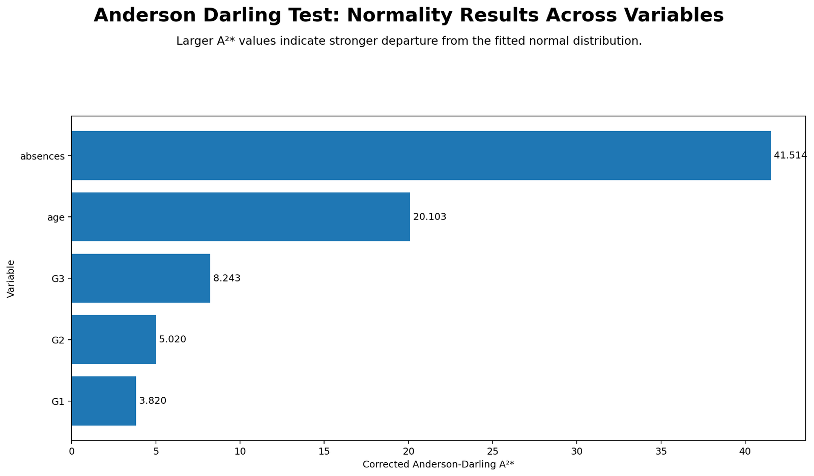
This chart compares Anderson Darling statistics across variables. Larger values indicate stronger departure from the selected reference distribution. This is important because normality is not a property of the whole dataset; it is specific to the variable or residual series being analyzed.
For example, a final grade variable may show different normality behavior than an absences variable. A count-like or skewed variable may produce a much larger Anderson Darling statistic because its distribution has tails or boundaries that differ from normality.
Decision/reporting conclusion: Use this chart to identify which variables need deeper normality review, transformation, robust analysis, or nonparametric alternatives.
Python Chart 6: Group AD Statistic Comparison
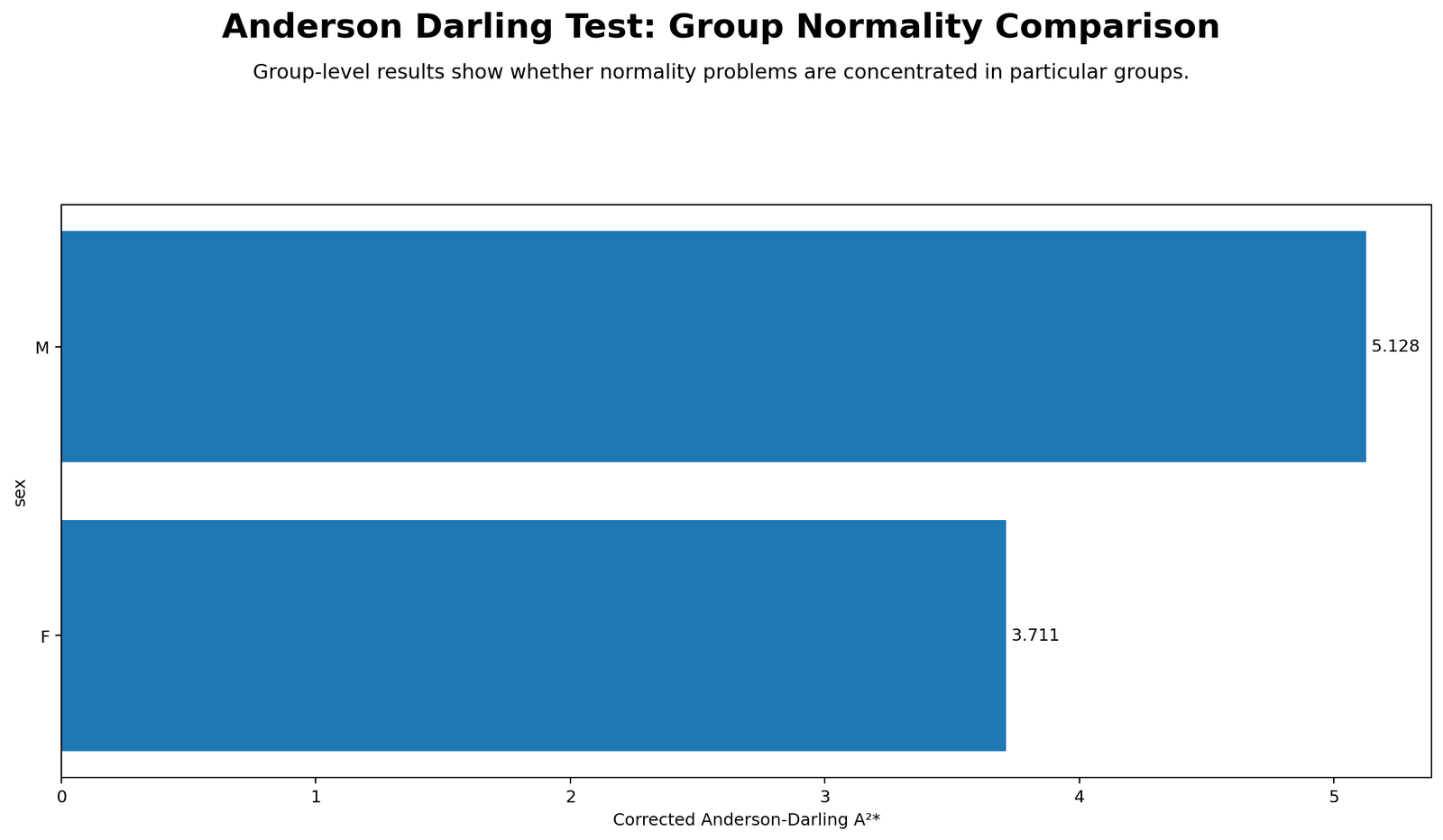
This chart compares Anderson Darling statistics across groups. A variable can be close to normal in one group but clearly non-normal in another. This matters for group comparisons, ANOVA, regression subgroup diagnostics and assumption reporting.
If one group has a much larger AD statistic, the analyst should inspect that group’s distribution separately. The issue may be a small subgroup sample size, outliers, ceiling effects, floor effects or true distributional difference.
Decision/reporting conclusion: Use this chart to decide whether normality concerns are general across the dataset or concentrated in particular groups.
R Chart-by-Chart Validation
The R charts validate the Python and SPSS Anderson Darling Test workflow using a separate analytical environment. The same six visual diagnostics are provided: distribution fit, normal Q-Q plot, empirical CDF versus fitted normal CDF, tail-weighted contributions, AD statistic across variables and group AD statistic comparison.
R Chart 1: Distribution Fit for Anderson Darling Test
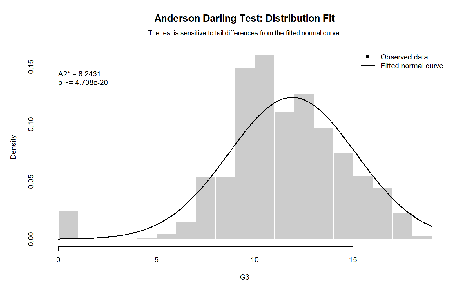
The R distribution fit chart validates the Python view of the observed sample shape. It shows whether the data follow the fitted normal curve or whether there are visible departures in the center, spread or tails. This provides a visual foundation for interpreting the Anderson Darling statistic.
Decision/reporting conclusion: Use this R chart to confirm whether the distribution fit pattern is reproducible across software workflows.
R Chart 2: Normal Q-Q Plot
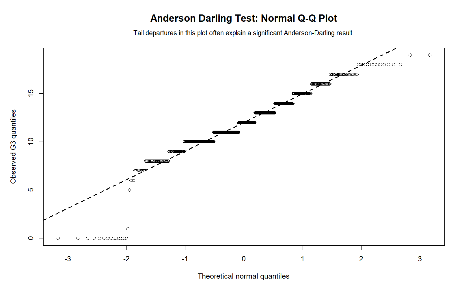
The R Q-Q plot validates the tail and quantile interpretation. If the points follow the diagonal line, the normality assumption looks more reasonable. If the points depart strongly at the ends, the Anderson Darling Test may detect non-normality because of tail mismatch.
Decision/reporting conclusion: Use this R Q-Q plot to confirm whether tail departures support the Anderson Darling result.
R Chart 3: Empirical CDF vs Fitted Normal CDF
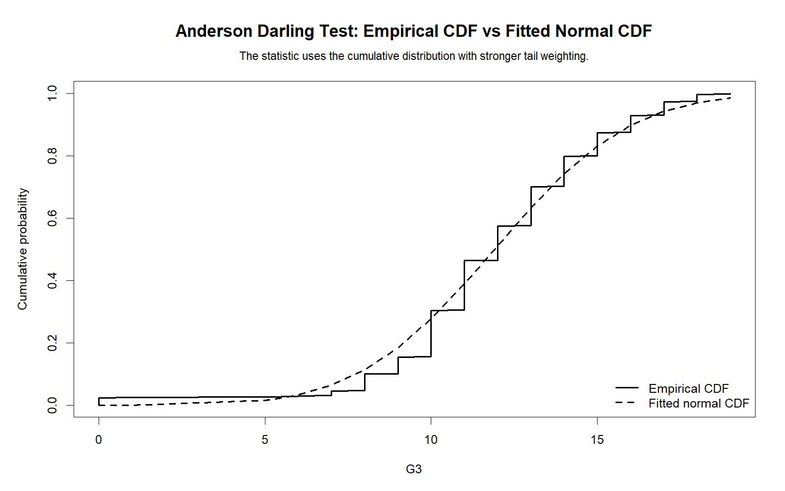
The R ECDF chart confirms the cumulative-distribution comparison. It shows how the observed cumulative distribution tracks or deviates from the fitted normal cumulative distribution. This chart is the bridge between visual distribution checking and the formal Anderson Darling formula.
Decision/reporting conclusion: Use this chart to explain whether the empirical cumulative pattern supports or contradicts the fitted normal reference.
R Chart 4: Tail-Weighted Contributions
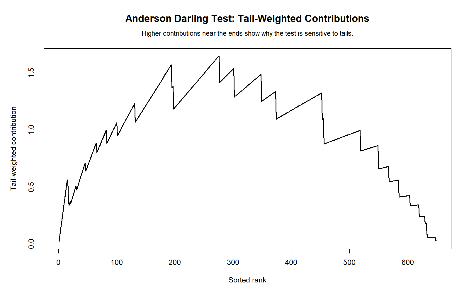
The R tail-weighted contribution chart confirms which portions of the distribution influence the Anderson Darling statistic most strongly. If the tails contribute heavily, the normality issue may involve outliers, heavy tails or skewed extremes rather than only central shape.
Decision/reporting conclusion: Use this chart to explain whether the Anderson Darling result is tail-driven and whether follow-up checks should focus on extreme values.
R Chart 5: Anderson Darling Statistic Across Variables
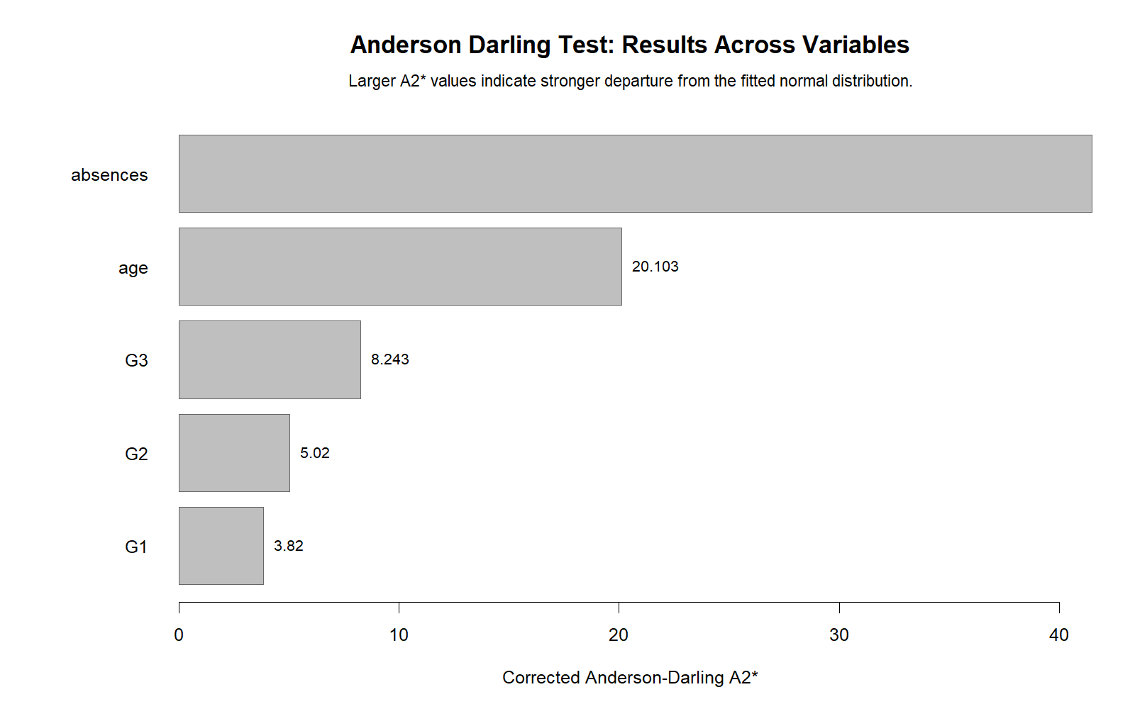
The R cross-variable chart validates which variables show the strongest departure from normality. Variables with higher AD statistics should receive closer attention in reports, especially if they are used in parametric tests, regression residual checks or confidence interval calculations.
Decision/reporting conclusion: Use this chart to prioritize which variables require transformation, robust methods or additional distribution diagnostics.
R Chart 6: Group AD Statistic Comparison
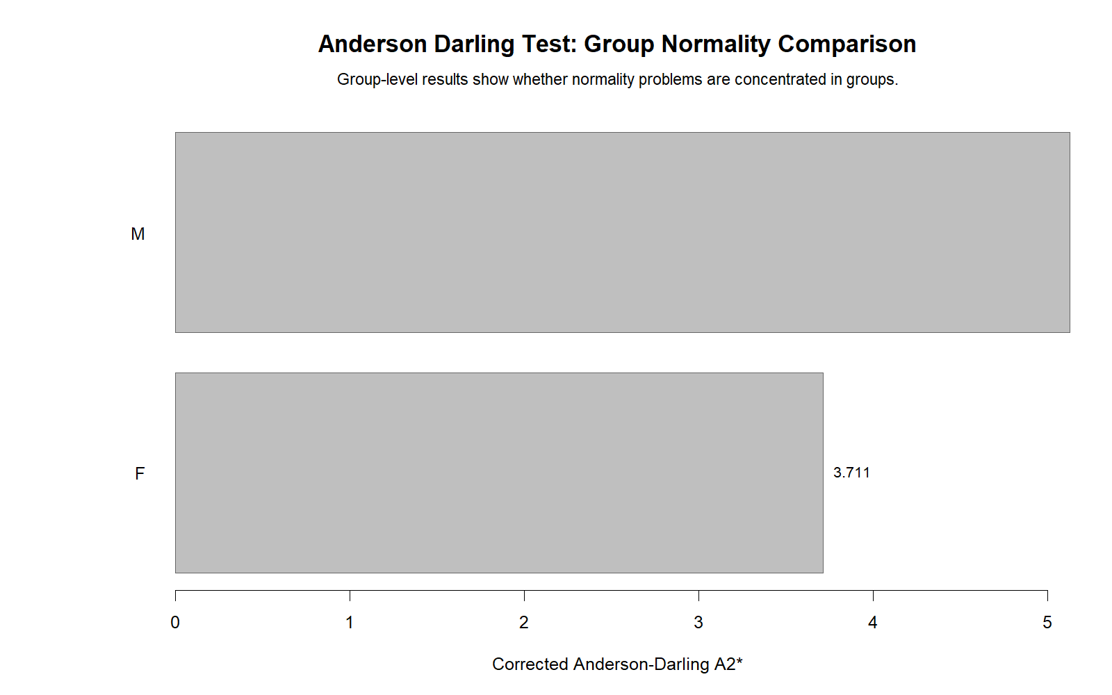
The R group comparison chart validates whether normality problems differ by subgroup. This is important when the next analysis compares groups or includes group predictors. If one group has a much larger Anderson Darling statistic, report that normality concerns may be group-specific.
Decision/reporting conclusion: Use this chart to decide whether normality is acceptable across all groups or whether subgroup-specific caution is needed.
Google AdSense in-content placement reserved here
SPSS, Python, R and Excel Workflows for the Anderson Darling Test
A complete Anderson Darling Test workflow includes a formal statistic and multiple charts. The analyst should not rely on one output table only. The best workflow includes descriptive statistics, distribution fit, Q-Q plot, empirical CDF comparison, tail-weighted contributions, and final p-value or critical-value decision.
SPSS Workflow
| Step | SPSS Action | Purpose |
|---|---|---|
| Open data | File > Open > Data | Load the SPSS-ready dataset. |
| Inspect distribution | Analyze > Descriptive Statistics > Explore | Request histogram, normality plots and descriptive output. |
| Run Anderson Darling workflow | Extension, custom syntax, R/Python integration or prepared output | Obtain AD statistic and p-value or critical-value decision. |
| Check Q-Q plot | Normal probability plot | Identify tail departures and quantile mismatch. |
| Export output | OUTPUT EXPORT or File > Export | Save SPSS PDF for reporting. |
Python Workflow
| Step | Python Action | Purpose |
|---|---|---|
| Read dataset | pandas.read_csv() | Load data into Python. |
| Select numeric variable | pd.to_numeric(), dropna() | Prepare clean data for the test. |
| Run Anderson Darling | scipy.stats.anderson() | Get AD statistic and critical values. |
| Create fitted distribution chart | matplotlib | Show observed distribution versus fitted normal curve. |
| Create Q-Q and ECDF charts | scipy, numpy, matplotlib | Explain quantile and cumulative-distribution fit. |
| Interpret tails | Tail contribution plot | Explain why the AD statistic is sensitive to extremes. |
R Workflow
| Step | R Action | Purpose |
|---|---|---|
| Read data | read.csv() | Import the dataset. |
| Select variable | na.omit() | Remove missing values. |
| Run Anderson Darling | nortest::ad.test() | Calculate statistic and p-value. |
| Create Q-Q plot | qqnorm(), qqline() or ggplot2 | Inspect normal quantile alignment. |
| Create ECDF chart | ecdf() | Compare empirical and fitted CDFs. |
| Compare variables/groups | Loop or grouped workflow | Identify variables or groups with larger AD statistics. |
Excel Workflow
| Excel Task | Formula or Method | Purpose |
|---|---|---|
| Sort values | Sort smallest to largest | Prepare ordered sample values. |
| Estimate mean | =AVERAGE(range) | Fit normal reference. |
| Estimate standard deviation | =STDEV.S(range) | Scale normal reference. |
| Fitted normal CDF | =NORM.DIST(x,mean,sd,TRUE) | Calculate theoretical cumulative probabilities. |
| Log terms | =LN(F) and =LN(1-F_reverse) | Build Anderson Darling statistic components. |
| AD statistic | Manual formula from sorted probabilities | Approximate A² statistic for learning and visualization. |
SPSS, Python, R and Excel Code for the Anderson Darling Test
SPSS Syntax for Anderson Darling Supporting Workflow
* Anderson Darling Test supporting normality workflow in SPSS.
* Replace G3 with your selected numeric variable.
* SPSS may require an extension, custom procedure, or R/Python integration for direct AD p-values.
TITLE "Anderson Darling Test Normality Workflow".
EXAMINE VARIABLES=G3
/PLOT BOXPLOT HISTOGRAM NPPLOT
/COMPARE GROUPS
/STATISTICS DESCRIPTIVES
/CINTERVAL 95
/MISSING LISTWISE
/NOTOTAL.
FREQUENCIES VARIABLES=G3
/STATISTICS=MEAN MEDIAN STDDEV SKEWNESS SESKEW KURTOSIS SEKURT MINIMUM MAXIMUM
/HISTOGRAM NORMAL
/ORDER=ANALYSIS.
* Optional: save standardized values for external Anderson Darling calculation.
DESCRIPTIVES VARIABLES=G3
/SAVE
/STATISTICS=MEAN STDDEV MIN MAX.
OUTPUT EXPORT
/CONTENTS EXPORT=VISIBLE
/PDF DOCUMENTFILE="Anderson-Darling-Test-SPSS-Output.pdf".Python Code for the Anderson Darling Test
import pandas as pd
import numpy as np
from scipy import stats
df = pd.read_csv("dataset.csv")
x = pd.to_numeric(df["G3"], errors="coerce").dropna().to_numpy()
# Anderson-Darling test for normality
ad_result = stats.anderson(x, dist="norm")
print("Anderson-Darling statistic:", ad_result.statistic)
print("Critical values:", ad_result.critical_values)
print("Significance levels:", ad_result.significance_level)
# Decision by critical values
for sig, crit in zip(ad_result.significance_level, ad_result.critical_values):
decision = "Reject normality" if ad_result.statistic > crit else "Do not reject normality"
print(f"{sig}% level: critical value={crit:.4f}; {decision}")
# Empirical CDF and fitted normal CDF for plotting
mu = np.mean(x)
sigma = np.std(x, ddof=1)
x_sorted = np.sort(x)
n = len(x_sorted)
empirical_cdf = np.arange(1, n + 1) / n
fitted_cdf = stats.norm.cdf(x_sorted, loc=mu, scale=sigma)
# Avoid exact 0 or 1 probabilities for log terms
eps = 1e-10
fitted_cdf_clipped = np.clip(fitted_cdf, eps, 1 - eps)
# Manual Anderson-Darling statistic for learning
i = np.arange(1, n + 1)
A2 = -n - np.mean((2 * i - 1) * (
np.log(fitted_cdf_clipped) +
np.log(1 - fitted_cdf_clipped[::-1])
))
print("Manual A-squared:", A2)R Code for the Anderson Darling Test
# Anderson Darling Test in R
# install.packages("nortest")
library(nortest)
df <- read.csv("dataset.csv")
x <- as.numeric(df$G3)
x <- na.omit(x)
# Anderson-Darling normality test
ad_result <- ad.test(x)
print(ad_result)
# Fitted normal parameters
mu <- mean(x)
sigma <- sd(x)
# Empirical CDF and fitted normal CDF
x_sorted <- sort(x)
n <- length(x_sorted)
empirical_cdf <- (1:n) / n
fitted_cdf <- pnorm(x_sorted, mean = mu, sd = sigma)
# Manual AD statistic for explanation
eps <- 1e-10
fitted_cdf <- pmin(pmax(fitted_cdf, eps), 1 - eps)
i <- 1:n
A2_manual <- -n - mean((2 * i - 1) * (
log(fitted_cdf) + log(1 - rev(fitted_cdf))
))
print(A2_manual)
# Q-Q plot
qqnorm(x)
qqline(x, col = "blue", lwd = 2)Excel Formulas for an Anderson Darling-Style Manual Check
Assume sorted values are in A2:A650.
Sample size:
=COUNT(A2:A650)
Mean:
=AVERAGE(A2:A650)
Standard deviation:
=STDEV.S(A2:A650)
Fitted normal CDF in B2:
=NORM.DIST(A2,$Mean_Cell$,$SD_Cell$,TRUE)
Reverse fitted normal CDF:
Use the fitted CDF value from the opposite end of the sorted list.
Log term for row i:
=LN(B2)+LN(1-Reversed_CDF)
Weighted term:
=(2*i-1)*Log_Term
Anderson-Darling statistic:
=-n-(1/n)*SUM(Weighted_Terms)
Decision:
Compare A² with Anderson Darling critical values or use SPSS, Python, or R for a formal p-value.APA Reporting Wording for the Anderson Darling Test
APA reporting for the Anderson Darling Test should include the test name, variable, statistic, p-value or critical-value decision, and interpretation. Because the Anderson Darling Test is tail-sensitive, a strong report should also mention Q-Q plot or tail-contribution evidence.
If the Anderson Darling Test Is Significant
The Anderson Darling Test indicated a significant departure from normality, A² = [value], p < .05. Therefore, the null hypothesis of normality was rejected. Visual inspection of the Q-Q plot and tail-weighted contribution chart suggested that the departure was influenced by distribution-tail mismatch.
If the Anderson Darling Test Is Not Significant
The Anderson Darling Test was not significant, A² = [value], p ≥ .05. Therefore, the test did not provide sufficient evidence to reject the normality assumption. The distribution fit chart, Q-Q plot and empirical CDF chart were also reviewed before making the final assumption decision.
Student-Friendly Reporting Sentence
The Anderson Darling Test was used because it is sensitive to tail deviations from normality. The result was interpreted with the p-value or critical-value decision and supported by the distribution fit chart, normal Q-Q plot and empirical CDF chart.
Common Mistakes in Anderson Darling Test Interpretation
| Mistake | Why It Is a Problem | Correct Practice |
|---|---|---|
| Ignoring tail sensitivity | Anderson Darling may reject normality because of tail mismatch. | Inspect the Q-Q plot and tail-weighted contribution chart. |
| Reporting only the statistic | A² alone does not explain whether the result is significant. | Report p-value or critical-value decision. |
| Calling it the same as Kolmogorov-Smirnov | KS and AD use different weighting and sensitivity. | Explain that AD gives more weight to tails. |
| Using it without visual checks | The test result does not show the shape of the problem. | Use histogram, Q-Q plot, ECDF and box plot. |
| Assuming nonsignificant means perfectly normal | Failure to reject normality is not proof of perfect normality. | Write that the test did not find sufficient evidence against normality. |
| Confusing normality with equal variance | AD tests distribution fit, not group variance equality. | Use Levene, Brown-Forsythe or Goldfeld-Quandt for variance issues. |
| Forgetting sample size | Large samples can detect small distribution departures. | Interpret statistical and practical significance together. |
Key reminder: The Anderson Darling Test is a strong normality diagnostic, but it should be used inside a complete assumption-checking workflow with Histogram Interpretation, Q-Q Plot Normality Check, P-P Plot Normality Check, and related tests such as Lilliefors Test.
When to Use the Anderson Darling Test
Use the Anderson Darling Test when you need a formal distribution-fit or normality test and tail behavior matters. It is especially useful when Q-Q plots suggest tail deviation, when outliers may affect normality, when the sample distribution appears close in the center but questionable in the tails, or when you want a stronger normality diagnostic than a basic distribution plot.
| Use Anderson Darling Test When | Reason | Related Guide |
|---|---|---|
| You need a normality test with tail sensitivity | AD gives more importance to lower and upper tail differences. | Q-Q Plot Normality Check |
| You compare empirical and fitted CDFs | AD is based on cumulative distribution differences. | Cramer-von Mises Test |
| You are checking assumptions before parametric tests | Normality affects many statistical procedures. | One-Tailed T Test |
| You suspect outliers or heavy tails | AD is sensitive to distribution tails. | Box Plot Interpretation |
| You need a complete normality report | AD complements KS, Lilliefors, Ryan-Joiner and Q-Q plots. | Ryan-Joiner Test |
If the Anderson Darling Test rejects normality, review sample size, tails, outliers, skewness, kurtosis, and the planned analysis. Possible follow-ups include transformation, robust methods, nonparametric methods, bootstrap confidence intervals, or practical reliance on the Central Limit Theorem when justified. For skewed variables, a guide such as Reciprocal Transformation may help.
Downloads and Resources for the Anderson Darling Test
The SPSS output PDF below supports the Anderson Darling Test workflow used in this guide. The Python and R charts provide visual evidence for distribution fit, Q-Q plot behavior, empirical CDF comparison, tail-weighted contributions, variable-level AD statistics and group-level AD statistics.
Download SPSS Output PDF
Verified SPSS output for the Anderson Darling Test normality and distribution-fit workflow.
Copy Anderson Darling Test Code
Use the SPSS, Python, R and Excel code blocks to reproduce the analysis.
Python Tail-Weighted Contributions Chart
Key visual showing why Anderson Darling is sensitive to tail departures.
R Normal Q-Q Plot
R validation chart for quantile and tail interpretation.
Related Internal Guides
Use these related Salar Cafe guides to connect the Anderson Darling Test with normality checks, distribution-fit tests, descriptive statistics, transformations, variance assumptions, regression diagnostics and reporting.
Cramer-von Mises Test
Kolmogorov-Smirnov Test
Lilliefors Test
Ryan-Joiner Test
Q-Q Plot Normality Check
Q-Q Plot Normality Check 2
P-P Plot Normality Check
Histogram Interpretation
Box Plot Interpretation
Descriptive Statistics
Frequency Distribution
Five Number Summary
Coefficient of Variation
Confidence Interval
Effect Size
Central Limit Theorem
Reciprocal Transformation
Levene Test
Brown-Forsythe Test
Cochran C Test
Goldfeld-Quandt Test
Ramsey RESET Test
Mauchly’s Test of Sphericity
Greenhouse-Geisser Correction
One-Tailed T Test
One Sample Z Test
One Proportion Z Test
Cross Tabulation
Clinical Trial Data Analysis Using R
FAQs About the Anderson Darling Test
What is the Anderson Darling Test?
The Anderson Darling Test is a goodness-of-fit test used to check whether sample data follow a specified distribution, most commonly the normal distribution.
What does the Anderson Darling Test measure?
It measures the weighted difference between the empirical distribution and the theoretical distribution, with extra weight given to the tails.
What is the Anderson Darling statistic?
The statistic is usually written as A². Larger A² values indicate stronger departure from the reference distribution.
What is the null hypothesis of the Anderson Darling Test?
The null hypothesis says that the sample data follow the selected theoretical distribution.
What is the alternative hypothesis of the Anderson Darling Test?
The alternative hypothesis says that the sample data do not follow the selected theoretical distribution.
How do I interpret a significant Anderson Darling Test?
If p < .05, reject the null hypothesis and conclude that the data differ significantly from the selected distribution.
How do I interpret a nonsignificant Anderson Darling Test?
If p ≥ .05, the test does not provide sufficient evidence to reject the selected distribution.
Is the Anderson Darling Test a normality test?
Yes, it is commonly used as a normality test, although it can also be used for other distribution-fit checks depending on software support.
How is Anderson Darling different from Kolmogorov-Smirnov?
The Kolmogorov-Smirnov Test focuses on the largest CDF gap, while Anderson Darling weights differences across the distribution and gives extra importance to the tails.
Why is Anderson Darling sensitive to tails?
Its formula uses logarithmic weighting of cumulative probabilities near 0 and 1, making tail deviations more influential.
Can I run the Anderson Darling Test in SPSS?
Yes, it can be supported through prepared output, extension workflows, custom procedures or external integration, while SPSS Explore plots can support the visual normality interpretation.
Can I run the Anderson Darling Test in Python?
Yes. Python can run the Anderson Darling Test with scipy.stats.anderson().
Can I run the Anderson Darling Test in R?
Yes. R can run the Anderson Darling Test with nortest::ad.test().
Can I calculate Anderson Darling in Excel?
Excel can be used to build a manual learning version of the statistic, but SPSS, Python or R are better for formal p-values and critical-value decisions.
Should I use charts with the Anderson Darling Test?
Yes. Use a distribution fit chart, Q-Q plot, empirical CDF chart and tail-weighted contribution chart to explain the result.
Google AdSense bottom placement reserved here
