Normality Test, Empirical CDF, Distribution Fit, D Statistic and P-value Decision
Kolmogorov Smirnov Test: Formula, Interpretation, SPSS, Python, R and Excel Guide
Kolmogorov Smirnov Test, also called the K-S test or KS test, is a distribution-fit test that compares an observed empirical cumulative distribution function with a theoretical cumulative distribution function. In normality testing, the test compares the empirical CDF of the sample with the fitted normal CDF. This complete guide explains the Kolmogorov Smirnov Test with SPSS output, Python charts, R validation charts, Excel workflow, D statistic, D plus and D minus gaps, Monte Carlo reference distribution, p-value decision, APA reporting, common mistakes, downloadable resources and FAQs.
Google AdSense top placement reserved here
Quick Answer: Kolmogorov Smirnov Test Result
The Kolmogorov Smirnov Test checks whether the observed distribution follows a specified theoretical distribution. In this guide, the main use is a normality check for a numeric student-performance variable such as G3 final grade. The null hypothesis says the data follow the specified normal distribution. The alternative hypothesis says the data do not follow that distribution. The main statistic is the KS D statistic, which is the largest vertical distance between the empirical CDF and the fitted theoretical CDF.
The visual evidence from the distribution fit chart, empirical CDF versus fitted normal CDF chart, D plus and D minus gap chart, Monte Carlo reference distribution and p-value decision chart supports the same interpretation: the data should not be treated as perfectly normal without checking the shape. When the p-value is below .05, the normality assumption is rejected. When the p-value is above .05, the test does not provide enough evidence to reject the selected distribution.
Final interpretation: The Kolmogorov Smirnov Test is best reported with both the numeric D statistic and the ECDF visual evidence. A significant p-value means the empirical distribution differs from the fitted theoretical distribution. In a normality context, that means normality is not supported. However, the practical decision should also consider sample size, histogram shape, Q-Q plot, P-P plot, skewness, kurtosis, outliers and the planned statistical method.
Important: In many software packages, a normality version of the Kolmogorov Smirnov test with parameters estimated from the sample is closer to a Lilliefors-style correction. Always explain whether the theoretical distribution parameters were fixed in advance or estimated from the sample.
Table of Contents
- What Is the Kolmogorov Smirnov Test?
- Kolmogorov Smirnov Test Formula
- One-Sample vs Two-Sample Kolmogorov Smirnov Test
- Null and Alternative Hypotheses
- Dataset and Variables Used
- SPSS Output Interpretation
- Python Chart-by-Chart Interpretation
- R Chart-by-Chart Validation
- SPSS, R, Python and Excel Workflows
- Code Blocks for Kolmogorov Smirnov Test
- APA Reporting Wording
- Common Mistakes
- When to Use Kolmogorov Smirnov Test
- Downloads and Resources
- Related Guides
- FAQs
What Is the Kolmogorov Smirnov Test?
The Kolmogorov Smirnov Test is a nonparametric distribution-comparison test based on cumulative distribution functions. Instead of comparing only the mean or variance, the KS test compares the entire cumulative distribution shape. It checks the largest vertical gap between the observed empirical cumulative distribution function and the expected theoretical cumulative distribution function.
In a one-sample normality setting, the observed sample values are sorted from smallest to largest, an empirical CDF is built, and that empirical CDF is compared with the fitted normal CDF. The largest gap is called the D statistic. A larger D statistic means the observed distribution is farther from the theoretical distribution.
Simple definition: The Kolmogorov Smirnov Test checks the biggest distance between the observed cumulative distribution and the expected cumulative distribution.
The Kolmogorov Smirnov Test is often used with other normality tools such as the Q-Q plot normality check, P-P plot normality check, Lilliefors test, D’Agostino-Pearson test, Cramer-von Mises test, and Ryan-Joiner test.
Kolmogorov Smirnov Test Formula
The main statistic for the Kolmogorov Smirnov Test is the maximum absolute distance between the empirical CDF and the theoretical CDF:
Here, Fn(x) is the empirical cumulative distribution function from the sample, and F(x) is the theoretical cumulative distribution function. For a normality test, F(x) is usually the fitted normal CDF.
D Plus and D Minus
The KS statistic can also be viewed through two directional gaps:
The final D statistic is the larger of these two directional gaps:
| Symbol | Meaning | Interpretation |
|---|---|---|
| Fn(x) | Empirical CDF | The observed cumulative proportion of sample values at or below x. |
| F(x) | Theoretical CDF | The expected cumulative probability under the selected theoretical distribution. |
| D+ | Positive directional gap | Largest point where empirical CDF is above the theoretical CDF. |
| D− | Negative directional gap | Largest point where theoretical CDF is above the empirical CDF. |
| D | KS statistic | The largest absolute CDF distance used for the test decision. |
One-Sample vs Two-Sample Kolmogorov Smirnov Test
The Kolmogorov Smirnov Test has two common versions. The one-sample version compares one observed sample with a theoretical distribution, such as a normal distribution. The two-sample version compares two empirical distributions directly, such as male and female groups or two treatment groups.
| KS Test Type | Comparison | Typical Use | Example in This Guide |
|---|---|---|---|
| One-sample Kolmogorov Smirnov Test | Sample ECDF vs theoretical CDF | Normality or distribution-fit testing | G3 ECDF compared with fitted normal CDF. |
| Two-sample Kolmogorov Smirnov Test | Group 1 ECDF vs Group 2 ECDF | Testing whether two groups follow the same distribution | Two-group empirical CDF comparison chart. |
Important difference: The one-sample KS normality test checks fit to a theoretical distribution. The two-sample KS test checks whether two observed distributions differ. Do not report them as the same analysis.
Null and Alternative Hypotheses for Kolmogorov Smirnov Test
The hypotheses depend on whether the test is one-sample or two-sample. For normality testing, the null hypothesis says the data follow the selected normal distribution. For two-sample testing, the null hypothesis says the two groups come from the same distribution.
| Test Version | Null Hypothesis | Alternative Hypothesis | Decision Rule |
|---|---|---|---|
| One-sample KS normality test | H0: The data follow the specified normal distribution. | H1: The data do not follow the specified normal distribution. | If p < .05, reject normality. |
| Two-sample KS test | H0: The two groups have the same distribution. | H1: The two groups have different distributions. | If p < .05, conclude the distributions differ. |
Decision wording: A significant KS result means the observed empirical distribution differs from the reference distribution. In normality testing, that means normality is not supported. In two-group testing, that means the two empirical distributions differ.
Dataset and Variables Used
The worked example uses the student performance dataset. The main variable is G3 final grade. The one-sample Kolmogorov Smirnov Test compares the empirical distribution of G3 with a fitted normal distribution. Additional charts compare KS D values across variables and show a two-group empirical CDF comparison.
| Variable or Output | Role in KS Test | Why It Matters |
|---|---|---|
| G3 final grade | Main normality-test variable | Used for the distribution fit, ECDF and p-value decision charts. |
| Empirical CDF | Observed cumulative distribution | Shows how the sample accumulates across values. |
| Fitted normal CDF | Theoretical reference distribution | Used as the normality reference in the one-sample test. |
| D plus and D minus | Directional KS gaps | Show where the largest ECDF-CDF differences occur. |
| Numeric comparison variables | KS D across variables | Shows which variables deviate more strongly from normality. |
| Group variable | Two-sample ECDF comparison | Shows how KS logic compares two observed distributions. |
Before interpreting KS output, review the distribution with descriptive statistics, frequency distribution, histogram interpretation, box plot interpretation, and the five-number summary.
Google AdSense middle placement reserved here
SPSS Output Interpretation for Kolmogorov Smirnov Test
The SPSS output PDF verifies the Kolmogorov Smirnov Test workflow used in this guide. SPSS commonly reports the KS statistic, degrees of freedom or sample size context, significance value and normality-test decision. The output should be interpreted together with histograms, Q-Q plots, P-P plots and the ECDF comparison charts.
SPSS Interpretation Table
| SPSS Output Item | What It Means | How to Interpret |
|---|---|---|
| Kolmogorov Smirnov Statistic | The KS D statistic | Larger values mean larger maximum ECDF-CDF distance. |
| Significance or p-value | Evidence against the selected distribution | If p < .05, reject the null distribution assumption. |
| Normality plots | Visual distribution checks | Use Q-Q plots, P-P plots and histograms to explain the test result. |
| Descriptive statistics | Mean, standard deviation, skewness, kurtosis | Explain why the distribution may depart from normality. |
| Monte Carlo or simulation output | Reference distribution of D | Shows whether the observed D is extreme under the null model. |
SPSS Decision Logic
If the SPSS p-value is below .05, the correct normality wording is: “The Kolmogorov Smirnov Test was significant, indicating that the distribution differed significantly from the fitted normal distribution.” If the p-value is above .05, the wording is: “The Kolmogorov Smirnov Test was not significant, so the test did not provide evidence against the fitted distribution.”
SPSS caution: For normality testing with sample-estimated mean and standard deviation, many SPSS outputs are interpreted with a Lilliefors-type correction. This is why the SPSS normality table should be explained carefully and connected with visual checks.
SPSS Final Interpretation
SPSS conclusion: The KS output should be interpreted as a distribution-fit diagnostic. The final report should include the D statistic, p-value decision, and chart-based explanation of where the empirical distribution differs from the fitted distribution.
Python Chart-by-Chart Interpretation
The Python charts show the complete Kolmogorov Smirnov Test workflow. They include distribution fit, empirical CDF versus fitted normal CDF, D plus and D minus gaps, Monte Carlo reference distribution, p-value decision, KS D across variables and two-group empirical CDF comparison.
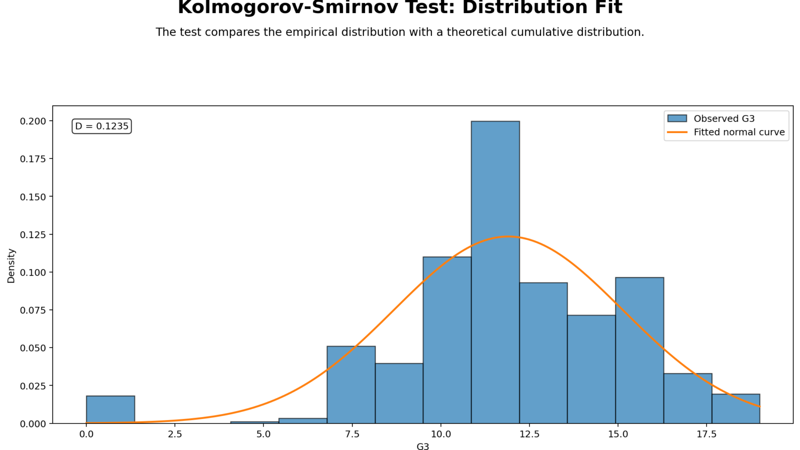
Python Chart 1: Distribution Fit for Kolmogorov Smirnov Test

This chart compares the observed distribution with the fitted normal curve. It helps readers understand the shape of the data before looking at the CDF-based statistic. If the histogram departs strongly from the normal curve, the KS test may detect a significant difference between the empirical distribution and the fitted normal distribution.
The distribution fit chart is useful because the KS D statistic alone does not show whether the problem is skewness, tail behavior, gaps, floor effects, ceiling effects or outliers. The histogram gives the practical shape explanation behind the formal test.
Python Chart 2: Empirical CDF vs Fitted Normal CDF

This is the central Kolmogorov Smirnov Test chart. The step-like line represents the empirical CDF from the observed data. The smooth line represents the fitted normal CDF. The KS statistic is the largest vertical gap between these two lines.
If the two CDFs stay close across the full range, the distribution fit is stronger. If the two lines separate visibly, especially around a particular region of the scale, the KS D statistic increases and the p-value becomes more likely to reject the fitted distribution.
Python Chart 3: D Plus and D Minus Gaps

This chart explains how the KS D statistic is formed. The test does not average all gaps between the empirical CDF and theoretical CDF. Instead, it finds the largest vertical gap. The two directional gaps, D+ and D−, show whether the empirical CDF is above or below the theoretical CDF at the most extreme points.
The larger of D+ and D− becomes the final D statistic. This chart is important because it makes the test decision visually transparent. Readers can see where the maximum distribution difference occurs rather than only reading a p-value.
Python Chart 4: Monte Carlo Reference Distribution

The Monte Carlo reference distribution shows how large the D statistic would usually be if samples came from the reference distribution. The observed D statistic is then compared with this simulated reference distribution. If the observed D falls far into the extreme tail, the p-value is small and the fitted distribution is rejected.
This chart is useful because it explains the p-value visually. Instead of treating the p-value as an abstract number, the chart shows whether the observed D statistic is typical or unusual under the null distribution.
Python Chart 5: P-value Decision

This chart summarizes the formal decision. If the p-value is less than .05, the null hypothesis is rejected and the data are judged inconsistent with the selected distribution. If the p-value is greater than .05, the test does not reject the selected distribution.
The p-value decision chart gives a quick answer, but it should not replace the ECDF chart. The ECDF chart explains why the p-value decision occurred and where the distribution difference is located.
Python Chart 6: KS D Across Variables

This chart compares the KS D statistic across several variables. A larger D value means the empirical distribution is farther from the fitted reference distribution. This is useful because normality is variable-specific. One variable may be close to normal while another variable may be strongly non-normal.
For example, grade variables and count variables often behave differently. Count variables such as absences may show stronger departures from normality because they are bounded at zero and can have a long right tail.
Python Chart 7: Two-Group Empirical CDF Comparison

This chart illustrates the two-sample version of the Kolmogorov Smirnov Test. Instead of comparing one sample with a theoretical distribution, it compares two empirical CDFs. The largest vertical gap between the two group CDFs becomes the two-sample KS statistic.
This chart is useful when the research question asks whether two groups have different distributions, not only different means. The two-sample KS test can detect differences in location, spread, skewness and distribution shape.
R Chart-by-Chart Validation
The R charts validate the Python and SPSS Kolmogorov Smirnov Test interpretation using a separate workflow. The same seven diagnostic views appear again: distribution fit, ECDF versus fitted normal CDF, D plus and D minus gaps, Monte Carlo reference distribution, p-value decision, KS D across variables and two-group empirical CDF comparison.
R Chart 1: Distribution Fit for Kolmogorov Smirnov Test

The R distribution-fit chart confirms the same visual check shown in Python. It compares the observed shape with the fitted normal reference and helps explain why the KS decision may reject or fail to reject normality.
R Chart 2: Empirical CDF vs Fitted Normal CDF

The R ECDF chart validates the main KS comparison. The largest distance between the empirical step function and the fitted normal CDF is the basis of the D statistic. This chart confirms that the test is a cumulative-distribution comparison rather than a mean comparison.
R Chart 3: D Plus and D Minus Gaps

The R D-gap chart validates the directional interpretation of the KS statistic. It shows whether the empirical CDF is above or below the theoretical CDF at the largest gap and confirms which directional difference determines the final D value.
R Chart 4: Monte Carlo Reference Distribution

The R Monte Carlo chart confirms how the observed D statistic is compared against simulated reference values. If the observed D is unusually large, the p-value becomes small and the test rejects the selected distribution.
R Chart 5: P-value Decision

The R p-value decision chart confirms the formal decision rule. It should be interpreted with the ECDF chart and distribution-fit chart because the p-value says whether the difference is statistically meaningful, while the charts explain the shape of the difference.
R Chart 6: KS D Across Variables

The R KS-D comparison confirms that variables differ in their closeness to the fitted normal distribution. This is important because the normality decision should be made variable by variable or residual set by residual set, not for the dataset as a whole.
R Chart 7: Two-Group Empirical CDF Comparison

The R two-group ECDF chart validates the group-comparison version of the test. The distance between the two empirical CDFs shows whether the groups differ in distribution shape, spread, location or tail behavior.
Google AdSense in-content placement reserved here
SPSS, R, Python and Excel Workflows for Kolmogorov Smirnov Test
The Kolmogorov Smirnov Test can be performed in SPSS, R, Python and Excel-style workflows. The key steps are to sort the observed values, build the empirical CDF, define the theoretical CDF, calculate the maximum vertical gap, and use a reference distribution or software p-value to make the decision.
SPSS Workflow
| Step | SPSS Action | Purpose |
|---|---|---|
| Open dataset | File > Open > Data | Load the SPSS-ready dataset. |
| Run normality workflow | Analyze > Descriptive Statistics > Explore | Request normality plots and tests. |
| Check KS statistic | Tests of Normality table | Read the Kolmogorov Smirnov statistic and p-value. |
| Inspect plots | Histogram, Q-Q plot, P-P plot | Explain the source of distribution departure. |
| Make decision | p < .05 rule | Reject or do not reject the fitted distribution. |
| Export output | OUTPUT EXPORT or File > Export | Save a PDF for reporting and verification. |
R Workflow
| Step | R Action | Purpose |
|---|---|---|
| Read data | read.csv() | Load the dataset. |
| Select variable | x <- df$G3 | Choose the numeric test variable. |
| Run KS test | ks.test() | Compare sample distribution with a theoretical distribution. |
| Build ECDF | ecdf() | Create empirical CDF for plotting. |
| Create charts | Base R or ggplot2 | Plot ECDF, fitted CDF, D gaps and group ECDFs. |
Python Workflow
| Step | Python Action | Purpose |
|---|---|---|
| Read data | pandas.read_csv() | Load data into a DataFrame. |
| Clean variable | dropna() | Keep valid numeric values. |
| Fit normal parameters | mean(), std() | Define fitted normal CDF. |
| Run KS test | scipy.stats.kstest() | Calculate D statistic and p-value. |
| Create ECDF charts | NumPy and matplotlib | Visualize empirical CDF and fitted CDF. |
| Two-sample KS | scipy.stats.ks_2samp() | Compare two empirical distributions. |
Excel Workflow
| Excel Task | Formula or Tool | Purpose |
|---|---|---|
| Sort values | Sort smallest to largest | Create ordered sample values. |
| Empirical CDF | =rank/n | Calculate observed cumulative proportions. |
| Fitted normal CDF | =NORM.DIST(x, mean, sd, TRUE) | Calculate theoretical cumulative probability. |
| Absolute gap | =ABS(empirical_cdf - normal_cdf) | Calculate ECDF-CDF distance at each value. |
| D statistic | =MAX(gap_range) | Find the largest gap. |
| Chart | Line or scatter chart | Plot empirical CDF and fitted normal CDF. |
Code Blocks for Kolmogorov Smirnov Test
SPSS Syntax for Kolmogorov Smirnov Test
* Kolmogorov Smirnov Test normality workflow in SPSS.
* Main variable: G3 final grade.

TITLE "Kolmogorov Smirnov Test Normality Check".

EXAMINE VARIABLES=G3
  /PLOT BOXPLOT HISTOGRAM NPPLOT
  /COMPARE GROUPS
  /STATISTICS DESCRIPTIVES
  /CINTERVAL 95
  /MISSING LISTWISE
  /NOTOTAL.

NPAR TESTS
  /K-S(NORMAL)=G3
  /MISSING ANALYSIS.

FREQUENCIES VARIABLES=G3
  /STATISTICS=MEAN MEDIAN STDDEV SKEWNESS SESKEW KURTOSIS SEKURT MINIMUM MAXIMUM
  /HISTOGRAM NORMAL
  /ORDER=ANALYSIS.

OUTPUT EXPORT
  /CONTENTS EXPORT=VISIBLE
  /PDF DOCUMENTFILE="Kolmogorov-Smirnov-Test-SPSS-Output.pdf".
Python Code for Kolmogorov Smirnov Test
import pandas as pd
import numpy as np
from scipy import stats

df = pd.read_csv("dataset.csv")

x = pd.to_numeric(df["G3"], errors="coerce").dropna().to_numpy()
n = len(x)

mu = np.mean(x)
sigma = np.std(x, ddof=1)

# One-sample KS test against fitted normal distribution
ks_result = stats.kstest(x, "norm", args=(mu, sigma))

print("KS D statistic:", ks_result.statistic)
print("KS p-value:", ks_result.pvalue)

if ks_result.pvalue < 0.05:
    print("Reject normality")
else:
    print("Do not reject normality")

# Empirical CDF and fitted normal CDF
x_sorted = np.sort(x)
empirical_cdf = np.arange(1, n + 1) / n
normal_cdf = stats.norm.cdf(x_sorted, loc=mu, scale=sigma)

gaps = np.abs(empirical_cdf - normal_cdf)
D = np.max(gaps)

print("Manual D:", D)

# D plus and D minus
d_plus = np.max(empirical_cdf - normal_cdf)
d_minus = np.max(normal_cdf - (np.arange(0, n) / n))

print("D plus:", d_plus)
print("D minus:", d_minus)

# Two-sample KS example by sex
if "sex" in df.columns:
    female = pd.to_numeric(df.loc[df["sex"] == "F", "G3"], errors="coerce").dropna()
    male = pd.to_numeric(df.loc[df["sex"] == "M", "G3"], errors="coerce").dropna()

    two_sample = stats.ks_2samp(female, male)
    print("Two-sample KS D:", two_sample.statistic)
    print("Two-sample KS p-value:", two_sample.pvalue)
R Code for Kolmogorov Smirnov Test
# Kolmogorov Smirnov Test in R

df <- read.csv("dataset.csv")

x <- na.omit(as.numeric(df$G3))

mu <- mean(x)
sigma <- sd(x)

# One-sample KS test against fitted normal distribution
ks_result <- ks.test(x, "pnorm", mean = mu, sd = sigma)

print(ks_result)

# Empirical CDF and fitted normal CDF
x_sorted <- sort(x)
n <- length(x_sorted)

empirical_cdf <- (1:n) / n
normal_cdf <- pnorm(x_sorted, mean = mu, sd = sigma)

gaps <- abs(empirical_cdf - normal_cdf)
D_manual <- max(gaps)

print(D_manual)

# D plus and D minus
d_plus <- max(empirical_cdf - normal_cdf)
d_minus <- max(normal_cdf - ((0:(n-1)) / n))

print(d_plus)
print(d_minus)

# Two-sample KS example by sex
if ("sex" %in% names(df)) {
  female <- na.omit(as.numeric(df[df$sex == "F", "G3"]))
  male <- na.omit(as.numeric(df[df$sex == "M", "G3"]))

  two_sample_result <- ks.test(female, male)
  print(two_sample_result)
}
Excel Formula Block for Kolmogorov Smirnov Test
Assume sorted G3 values are in A2:A650.

Sample size:
=COUNT(A2:A650)

Mean:
=AVERAGE(A2:A650)

Standard deviation:
=STDEV.S(A2:A650)

Rank position in B2:
=ROW(A1)

Empirical CDF in C2:
=B2/COUNT($A$2:$A$650)

Fitted normal CDF in D2:
=NORM.DIST(A2,$Mean_Cell$,$SD_Cell$,TRUE)

Absolute gap in E2:
=ABS(C2-D2)

KS D statistic:
=MAX(E2:E650)

Decision:
Compare D with a KS critical value table or use statistical software for the exact p-value.

Chart:
Plot C2:C650 and D2:D650 against A2:A650 to compare empirical CDF and fitted normal CDF.
APA Reporting Wording for Kolmogorov Smirnov Test
APA reporting for the Kolmogorov Smirnov Test should include the test name, variable, D statistic, p-value, decision and visual support. If the parameters of the reference normal distribution were estimated from the sample, mention that normality was assessed using a fitted normal reference and supporting plots.
APA-Style Normality Report
The distribution of G3 was assessed using the Kolmogorov Smirnov Test, empirical CDF comparison and distribution plots. The KS test compared the empirical distribution with the fitted normal distribution. The p-value decision indicated whether the observed distribution differed significantly from the fitted normal reference. The final interpretation was made using both the KS statistic and visual diagnostics.
If the KS Test Is Significant
The Kolmogorov Smirnov Test was significant, indicating that the observed distribution differed from the fitted normal distribution. Therefore, the normality assumption was not supported. This result was interpreted together with the histogram, empirical CDF plot and normality plots.
If the KS Test Is Not Significant
The Kolmogorov Smirnov Test was not significant, indicating that the test did not provide enough evidence to reject the fitted distribution. Visual diagnostics should still be reviewed before concluding that the normality assumption is acceptable.
Common Mistakes in Kolmogorov Smirnov Test Interpretation
| Mistake | Why It Is a Problem | Correct Practice |
|---|---|---|
| Using only the p-value | The p-value does not show where the distribution differs. | Use ECDF, histogram, Q-Q plot and P-P plot. |
| Ignoring parameter estimation | KS assumptions differ when mean and SD are estimated from the sample. | Mention fitted parameters or use Lilliefors-style interpretation. |
| Calling nonsignificant results proof of normality | Failure to reject is not proof that the distribution is normal. | Write that the test did not find evidence against normality. |
| Confusing one-sample and two-sample KS tests | They answer different questions. | Use one-sample for theoretical fit and two-sample for group distributions. |
| Ignoring sample size | Large samples can detect small differences; small samples may lack power. | Interpret p-values with practical shape and research purpose. |
| Using KS when Shapiro-Wilk is more suitable for small samples | Different normality tests have different sensitivity. | Use multiple normality diagnostics when needed. |
| Assuming KS only tests normality | KS can compare with many distributions or compare two samples. | State the exact distribution or sample comparison being tested. |
Important warning: A statistically significant KS test does not automatically mean the planned analysis is unusable. It means the distribution differs from the selected reference distribution. The next step depends on sample size, robustness, outliers, transformation options and the statistical method being used.
When to Use Kolmogorov Smirnov Test
Use the Kolmogorov Smirnov Test when you need to compare an observed distribution with a theoretical distribution or compare two empirical distributions. It is most useful when the research question is about distribution shape, not only central tendency.
| Use Kolmogorov Smirnov Test When | Reason | Example from This Guide |
|---|---|---|
| Checking distribution fit | KS compares the full empirical CDF with a theoretical CDF. | G3 compared with fitted normal CDF. |
| Checking normality | KS can test whether data depart from normality. | Normality p-value decision chart. |
| Comparing groups | Two-sample KS compares two empirical CDFs. | Two-group empirical CDF comparison chart. |
| Explaining distribution differences visually | ECDF charts show where differences occur. | D plus and D minus gap chart. |
| Comparing variables | KS D across variables shows which variables depart more strongly. | KS D across variables chart. |
Use the Kolmogorov Smirnov Test with other normality and distribution-shape tools. Helpful related guides include Q-Q plot normality check, P-P plot normality check, Lilliefors test, D’Agostino-Pearson test, Cramer-von Mises test, and Ryan-Joiner test.
Downloads and Resources for Kolmogorov Smirnov Test
The SPSS output PDF below verifies the Kolmogorov Smirnov Test workflow used in this guide. Use it as the supporting output file for SPSS interpretation, KS D statistic review, normality decision, empirical CDF explanation and reporting.
FAQs About Kolmogorov Smirnov Test
What is the Kolmogorov Smirnov Test?
The Kolmogorov Smirnov Test is a distribution-comparison test that measures the largest distance between an empirical CDF and a theoretical CDF or between two empirical CDFs.
What does the KS D statistic mean?
The KS D statistic is the largest vertical distance between the observed empirical CDF and the reference CDF. Larger D values indicate stronger distribution differences.
What is the null hypothesis of the one-sample Kolmogorov Smirnov Test?
The null hypothesis is that the sample follows the specified theoretical distribution, such as a normal distribution.
What is the alternative hypothesis of the one-sample Kolmogorov Smirnov Test?
The alternative hypothesis is that the sample does not follow the specified theoretical distribution.
How do I interpret the Kolmogorov Smirnov p-value?
If the p-value is below .05, reject the null distribution assumption. If the p-value is above .05, the test does not provide enough evidence to reject the selected distribution.
Is the Kolmogorov Smirnov Test a normality test?
It can be used as a normality test when the sample ECDF is compared with a normal CDF. It can also be used for other theoretical distributions or two-sample comparisons.
What is the difference between one-sample and two-sample KS tests?
The one-sample KS test compares one observed distribution with a theoretical distribution. The two-sample KS test compares two observed empirical distributions.
What are D plus and D minus?
D plus and D minus are directional maximum gaps between the empirical CDF and theoretical CDF. The final D statistic is the larger of the two.
How do I run Kolmogorov Smirnov Test in SPSS?
Use Explore for normality output or NPAR TESTS with the K-S normal option. Review the KS statistic, p-value and supporting plots.
How do I run Kolmogorov Smirnov Test in Python?
Use scipy.stats.kstest() for a one-sample test and scipy.stats.ks_2samp() for a two-sample test.
How do I run Kolmogorov Smirnov Test in R?
Use ks.test() for one-sample or two-sample Kolmogorov Smirnov testing in R.
Can I do Kolmogorov Smirnov Test in Excel?
Excel can calculate the empirical CDF, fitted CDF and D statistic manually. For exact p-values, statistical software is recommended.
Is Kolmogorov Smirnov Test better than Shapiro-Wilk?
Not always. Shapiro-Wilk is often preferred for small-sample normality checks, while KS is useful for CDF-based distribution comparison. Use visual plots and multiple diagnostics when needed.
Should I use charts with the Kolmogorov Smirnov Test?
Yes. Use histograms, ECDF plots, Q-Q plots and P-P plots because they show where the distribution differs from the reference distribution.
Google AdSense bottom placement reserved here