
Page’s Trend Test: Formula, Interpretation, Python, R, SPSS and Excel Guide
Page’s trend test, also called Page’s test for ordered alternatives, is a rank-based procedure for detecting a prespecified monotonic pattern across three or more related conditions. This complete guide explains the hypotheses, Page L statistic, large-sample standardization, assumptions, worked grade example, chart interpretation, and reproducible analysis in Python, R, SPSS and Excel.
A priori order
One-sided trend
Average ranks for ties
Python + R + SPSS + Excel
The grades show a statistically significant ordered increase from G1 to G2 to G3.
For 649 students observed at three ordered grade occasions, Page’s trend test produced L = 8,164. Under the supplied large-sample reference, the null expectation was E(L) = 7,788, the null variance was 1,298, and the standardized statistic was z = 10.436. The one-sided probability was p = 8.4556 × 10⁻²⁶, far below α = .05. The prespecified null hypothesis of no increasing order is therefore rejected.
The condition mean ranks were 1.761 for G1, 1.898 for G2 and 2.341 for G3. Raw means also rose from 11.399 to 11.570 to 11.906, while medians were 11, 11 and 12. These summaries support the same directional story, but the formal inference comes from blockwise ranks and the prespecified G1 < G2 < G3 order.
What does Page’s trend test measure?
A directional rank trend across related conditions whose order was specified before analyzing the outcomes.
Page’s trend test asks whether repeated conditions tend to follow a particular monotonic order. It is not merely a test that the conditions differ. The method gives extra weight to observations that occupy higher ranks at later, stronger or otherwise higher-scored conditions, making it especially useful when theory predicts a sequence such as low dose < medium dose < high dose or baseline < interim < final.
The statistical target
Suppose every participant is measured under k conditions. The observations are ranked within each participant, not pooled down the columns. The rank totals are then weighted by scores representing the prespecified condition order. A large Page L statistic occurs when high within-block ranks repeatedly fall in conditions assigned larger order scores.
The null hypothesis is exchangeability across condition labels within each block: there is no consistent tendency for the ranks to increase according to the stated order. The ordered alternative says that the population responses progress in that direction. Because the alternative is directional, the usual test is one-sided.
What it does not establish
Page’s trend test does not estimate a regression slope, a mean change per occasion, or the probability that every participant improves. It does not identify which individual transitions differ, and it does not automatically provide post hoc pairwise comparisons. It also does not justify selecting the order after inspecting the sample means.
When the goal is simply to detect any difference among repeated conditions without an ordered prediction, use the Friedman test. When the goal is to quantify overall rank agreement, report Kendall’s W. When the conditions are independent groups, an ordered test such as the Jonckheere-Terpstra test is more appropriate.
When should you use Page’s trend test?
Use it when the blocks are related, the conditions are ordered in advance and the scientific alternative is monotonic.
A defensible Page’s trend test begins with study design. Non-normality alone is not enough. The method is selected because the same blocks appear under all conditions and because the researcher has a meaningful directional sequence before seeing the results.
Confirm related conditions
Every student, patient, site or matched block contributes one value to each occasion.
Prespecify the order
Define the expected sequence from theory, protocol, dose or time before testing.
Rank within blocks
Convert each row to ascending ranks and use average ranks for ties.
Weight rank totals
Multiply each condition rank sum by its ordered score and add the products.
Use the upper tail
Large L supports the increasing alternative; reverse scores for a decreasing prediction.
Good applications
Choose another method when
Use a sign test or paired Wilcoxon method for only two related conditions. Use Friedman when no direction was prespecified. Use repeated-measures ANOVA when parametric modeling is appropriate, and consider mixed-effects regression for incomplete follow-up, covariates, interactions or irregular timing.
For independent ordered groups, Page’s trend test is structurally wrong because the rows are not shared blocks. Consider Jonckheere-Terpstra, an ordinal model or a planned regression trend instead. For binary repeated outcomes, Cochran’s Q addresses an omnibus difference, but an ordered binary trend requires a test designed for that outcome.
Why can Page’s trend test be more focused than Friedman?
Friedman spreads its sensitivity across all possible departures from equality. Page’s trend test concentrates evidence in one prespecified direction. When the order is scientifically correct, that focus can improve power. The tradeoff is that an unexpected nonmonotonic pattern may produce a significant Friedman result but weak Page evidence. Direction should therefore come from the research question, not from whichever arrangement makes L largest.
How Page’s trend test works
The method can be reconstructed from six transparent operations.
The computational logic of Page’s trend test is simple enough to audit by hand for a small dataset and stable enough to automate for hundreds of blocks.
1. Arrange a complete matrix
Rows represent independent blocks and columns represent conditions in the exact hypothesized order. In the example, one row is one student and the columns are G1, G2 and G3.
2. Rank each row
The smallest value receives rank 1 and the largest receives rank k. Tied values receive their average rank. For 12, 12, 13, the ranks are 1.5, 1.5 and 3.
3. Sum each condition
Add the within-row ranks down each column. The verified rank sums are 1,143 for G1, 1,232 for G2 and 1,519 for G3.
4. Apply order scores
Use scores 1, 2 and 3 for G1, G2 and G3. Multiply each condition rank sum by its score. Larger scores reward high ranks appearing later in the hypothesized sequence.
5. Standardize L
Compare the observed Page L with its null mean and variance. For large samples, convert the difference to a normal z statistic and calculate the upper-tail probability.
6. Interpret with raw data
Report the rank pattern, but also show means, medians, interquartile ranges and individual direction counts. Rank significance alone does not communicate practical magnitude.
Variables and data dictionary for the worked analysis
The example uses three grades from the same 649 students.
The worked Page’s trend test uses the same student-performance data structure throughout Python, R, SPSS and Excel. Keeping the variable definitions identical is essential for software agreement.
| Variable | Role | Scale and coding | Observed summary | Interpretive purpose |
|---|---|---|---|---|
| student / block | Repeated-measures identifier | One unique row per student | 649 complete blocks | Maintains dependence within students and independence between students |
| G1 | First ordered occasion | Numeric grade, 0-20 | Mean 11.399; median 11; IQR 10-13 | Receives order score 1 |
| G2 | Second ordered occasion | Numeric grade, 0-20 | Mean 11.570; median 11; IQR 10-13 | Receives order score 2 |
| G3 | Third ordered occasion | Numeric grade, 0-20 | Mean 11.906; median 12; IQR 10-14 | Receives order score 3 |
| within-row ranks | Analysis transformation | Ranks 1 to 3; averages for ties | Mean ranks 1.761, 1.898, 2.341 | Removes reliance on raw-score normality while preserving order |
Complete-block requirement
The analysis contains 649 usable rows because every included student has G1, G2 and G3. A simple complete-block implementation ordinarily removes any row missing one of the three values. That rule should be stated because different missing-data choices can change rank totals, Page L and the estimand.
Listwise deletion is straightforward but not always harmless. When missingness is substantial, a longitudinal model may be preferable. The supplied workbook is internally consistent because the same 649 rows appear in the raw-data, working, calculation and reporting sheets.
Outcome scale
The method requires observations that can be ordered meaningfully. Numeric grades qualify, and many ordinal ratings also qualify. The distances between grades do not need to be normally distributed because Page’s trend test uses ranks, but the conditions should measure the same construct on a comparable scale.
A changed exam, grading policy or measurement instrument can create an apparent trend that is partly methodological. Statistical significance should be interpreted alongside the study protocol and educational context.
Page’s trend test hypotheses and directional order
The order is part of the hypothesis and must be fixed before seeing the outcomes.
The distinctive feature of Page’s trend test is the ordered alternative. The procedure is not a post hoc search over every possible permutation of the condition labels.
Null hypothesis
H₀: the repeated condition distributions do not show the prespecified monotonic ordering. Under the randomization interpretation, condition labels are exchangeable within each block with respect to the linear rank score.
The null does not require that every raw observation be identical across conditions. It says that the systematic rank alignment with the specified order is absent.
Ordered alternative
H₁: responses tend to increase according to G1 < G2 < G3. Larger values should occur more often at conditions with larger order scores.
For a decreasing alternative, reverse the columns or use scores that run in the opposite direction. Do not run both directions and report only the smaller one-sided p-value without accounting for that choice.
Use scores 1, 2, …, k and the upper tail. Large L supports the prediction.
Reverse the condition order or scores before calculation, then use the upper tail for the reversed sequence.
Use Friedman or another two-sided/global method rather than inventing an order after inspection.
Page’s trend test formula
Rank sums are multiplied by order scores, then standardized against the null reference.
The formula for Page’s trend test is compact. Let b denote the number of complete blocks, k the number of ordered conditions, Rj the sum of within-block ranks for condition j, and j the score attached to its position in the predicted sequence.
For the increasing order, each condition rank sum is weighted by 1, 2, …, k. Larger L indicates stronger alignment between high ranks and later ordered conditions.
This is the conventional null expectation used in the supplied Python, R and Excel audit.
This large-sample variance yields the standard normal approximation used in the verified reports. Conditional permutation implementations can preserve observed tie structures directly.
The increasing alternative uses the upper normal tail. A one-sided p-value is appropriate only because the order was specified in advance.
Worked Page’s trend test example
A complete calculation using 649 students measured at G1, G2 and G3.
The worked Page’s trend test evaluates an a priori increasing order across three grades. Each student is a block, so the method compares a student’s three grades only with one another when assigning ranks.
Illustrative row ranking
| G1 | G2 | G3 | Ranks | Row contribution to L |
|---|---|---|---|---|
| 0 | 11 | 11 | 1, 2.5, 2.5 | 1(1)+2(2.5)+3(2.5)=13.5 |
| 12 | 13 | 12 | 1.5, 3, 1.5 | 1.5+6+4.5=12 |
| 15 | 16 | 17 | 1, 2, 3 | 1+4+9=14 |
| 14 | 14 | 14 | 2, 2, 2 | 2+4+6=12 |
A perfectly increasing row contributes 14, while an all-tied row contributes the null-centered value of 12. The full statistic adds these weighted rank contributions across all 649 students.
Verified final result
The observed statistic is 376 points above its null expectation. Relative to the reference standard deviation √1,298 = 36.028, this produces z = 10.436.
Reject H₀ at α = .05
The probability of an L value at least this large under the stated asymptotic null is approximately 8.46 × 10⁻²⁶.
Pattern counts
Exactly 398 students had G1 ≤ G2 ≤ G3, while 251 had another pattern. Of the full sample, 95 students showed a strictly increasing sequence and 89 had all three grades equal.
Adjacent transitions
For G2-G1, 273 students increased, 187 decreased and 189 tied. For G3-G2, 290 increased, 72 decreased and 287 tied. Both adjacent sign-test summaries favor the planned direction.
Omnibus support
Friedman’s χ²(2) was 167.328 with p ≈ 4.63 × 10⁻³⁷. Kendall’s W was 0.1289, indicating modest overall rank concordance despite the extremely small p-value from the large sample.
Python charts for Page’s trend test
Five visual checks connect the final statistic to rank sums, student patterns and source values.
The Python output for Page’s trend test presents the same verified numbers from several perspectives. Each chart answers a different audit question and should be interpreted with its scale in mind.
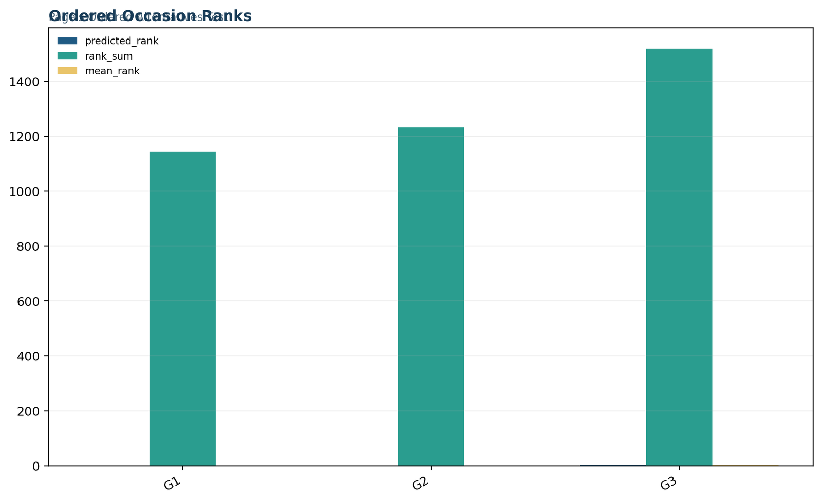
Python chart 1: ordered occasion ranks
The column rank sums rise from 1,143 to 1,232 to 1,519. Because the bars share a scale dominated by rank sums, the predicted-order and mean-rank series appear close to the baseline. Read the exact mean ranks as 1.761, 1.898 and 2.341. The dominant visual message is that G3 accumulated substantially more high within-student ranks than G1 or G2.
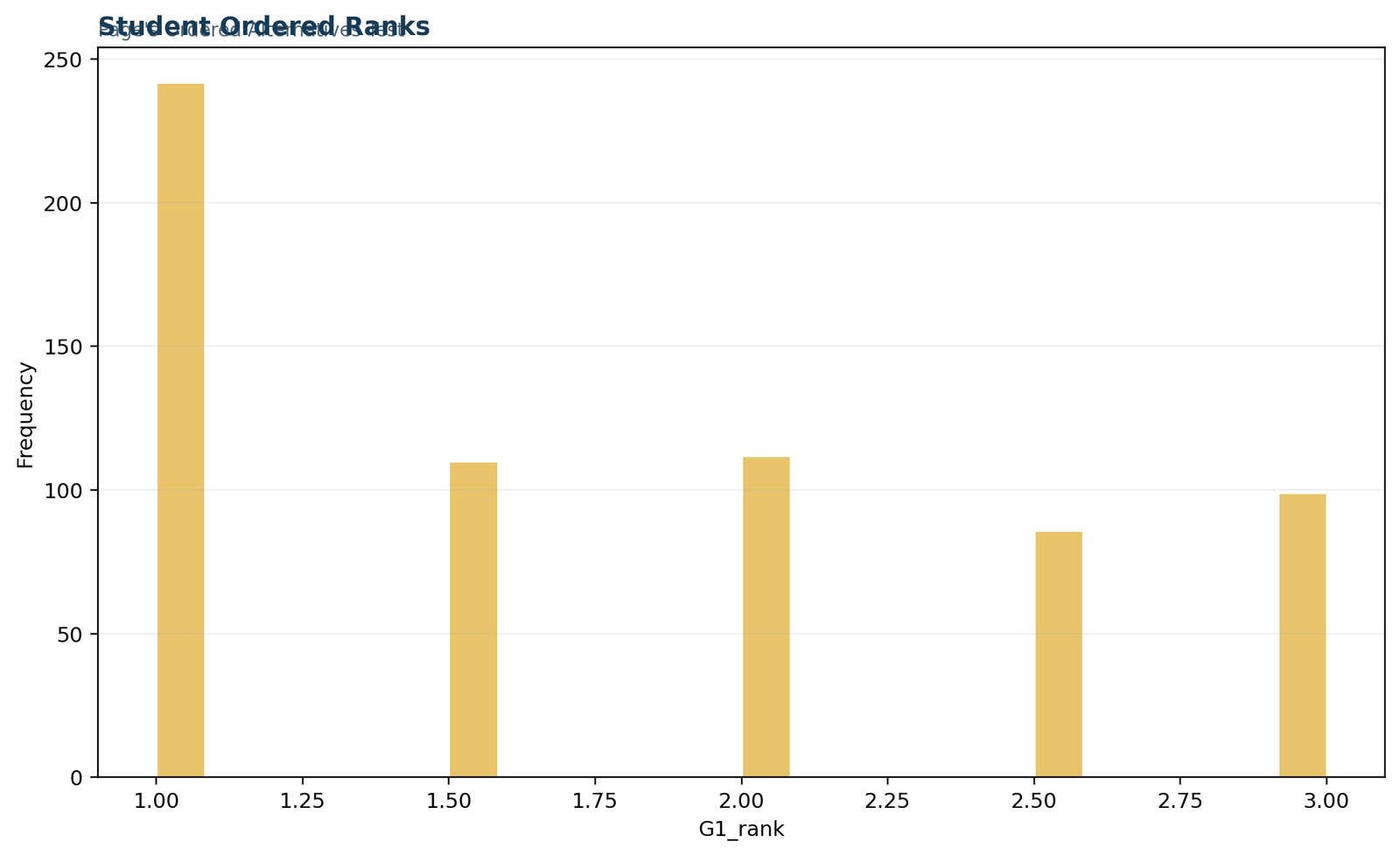
Python chart 2: student ordered ranks
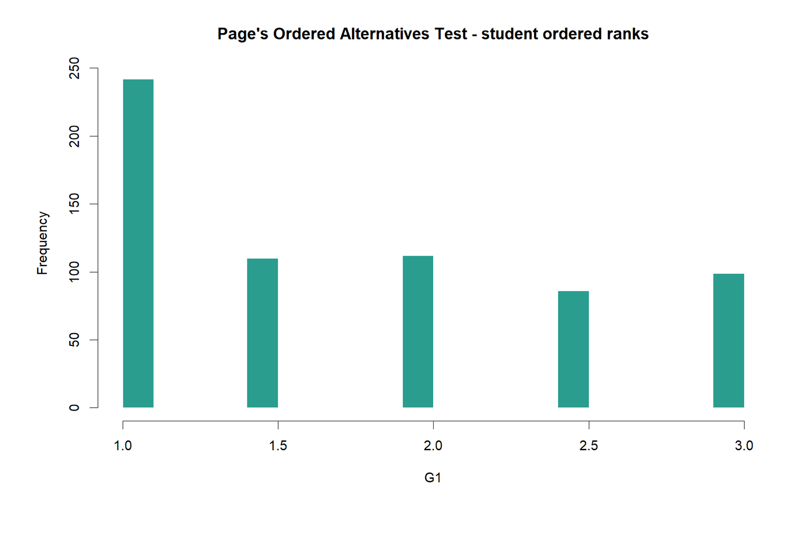
This frequency chart displays how often G1 occupied each possible average-rank value. G1 received rank 1 for 242 students, rank 1.5 for 110, rank 2 for 112, rank 2.5 for 86 and rank 3 for 99. The concentration toward lower ranks helps explain why G1 has the smallest condition mean rank, but the formal Page statistic uses all three condition rank columns.
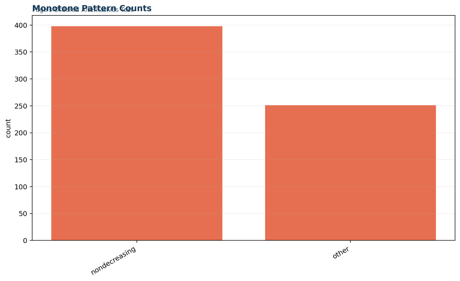
Python chart 3: monotone pattern counts
The plot separates 398 nondecreasing G1 ≤ G2 ≤ G3 rows from 251 other rows. This simple count is easy to understand and agrees with the directional conclusion, yet it is not the Page statistic. Page’s trend test uses the degree and placement of within-row ranks, allowing partially ordered rows and ties to contribute more information than a binary pattern label.
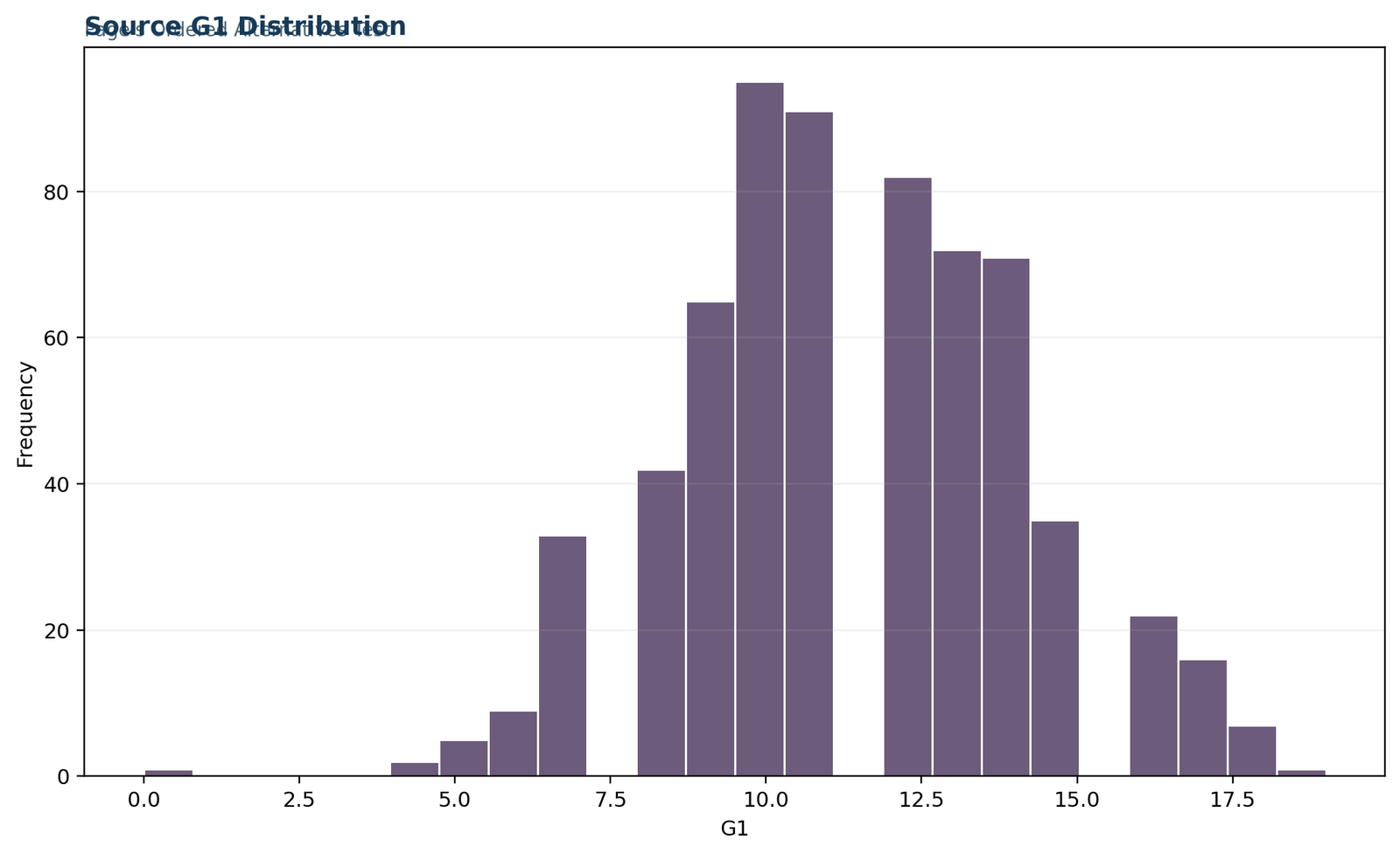
Python chart 4: source G1 distribution
The baseline grade distribution spans 0 to 19 and is concentrated around 9 to 14. This chart verifies that the source is discrete and contains many repeated values, which explains the frequency of tied within-student ranks. It provides context for the outcome scale but cannot by itself establish an ordered repeated-measures trend.
Python chart 5: verified result summary
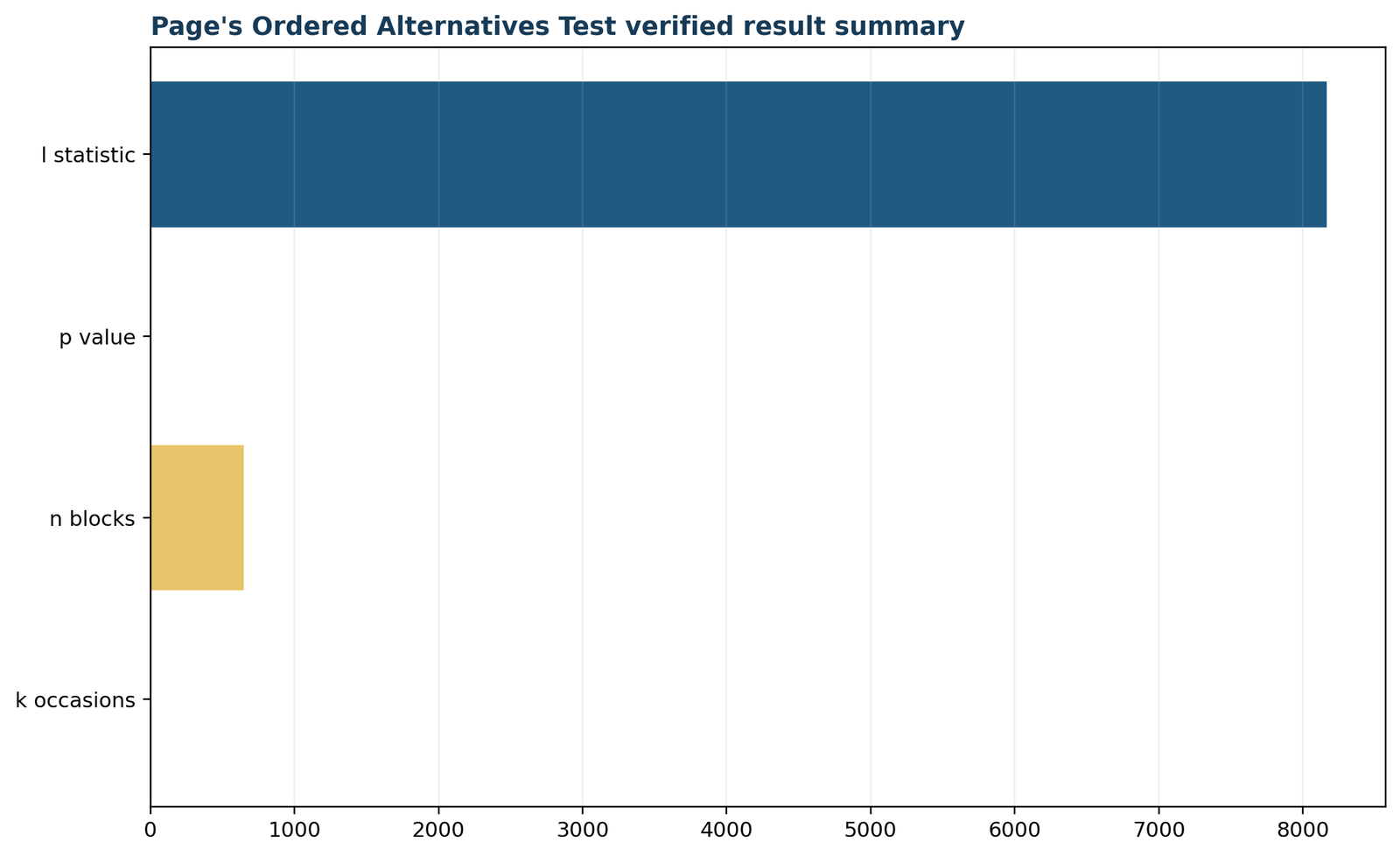
The summary places L = 8,164, p = 8.4556 × 10⁻²⁶, n = 649 and k = 3 on one numeric axis. The p-value and number of occasions are visually compressed because L is thousands of units. Use the chart as a verification dashboard, not as a comparison of commensurate magnitudes. The exact labels in the report are the authoritative reading.
R charts for Page’s trend test
The R report independently reproduces the primary statistic, ordered ranks and standardization.
The R charts confirm that Page’s trend test was reconstructed independently rather than copied from the Python output. Small display differences reflect plotting choices, while the underlying values agree.
R chart 1: primary metrics
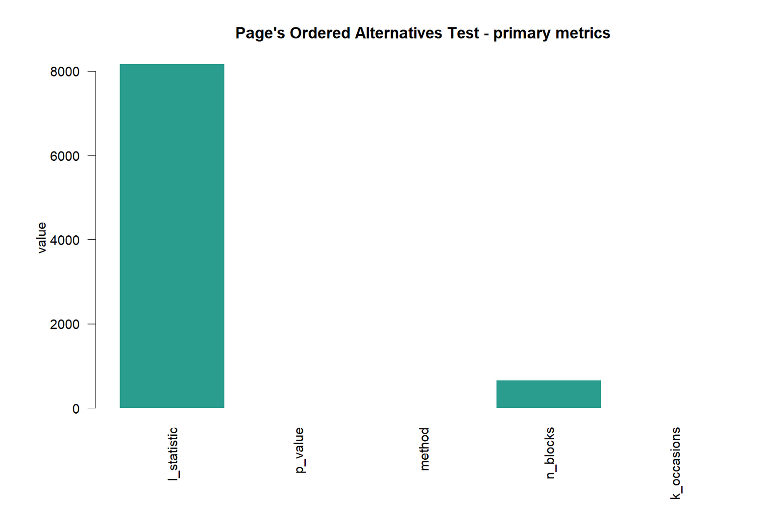
The plot includes L, p, method coding, n blocks and k occasions. L dominates at 8,164 and n is visible at 649; the tiny p-value and small k are compressed. The chart verifies inclusion of all primary report fields, but it should be read alongside the numerical result summary.
R chart 2: ordered occasion ranks
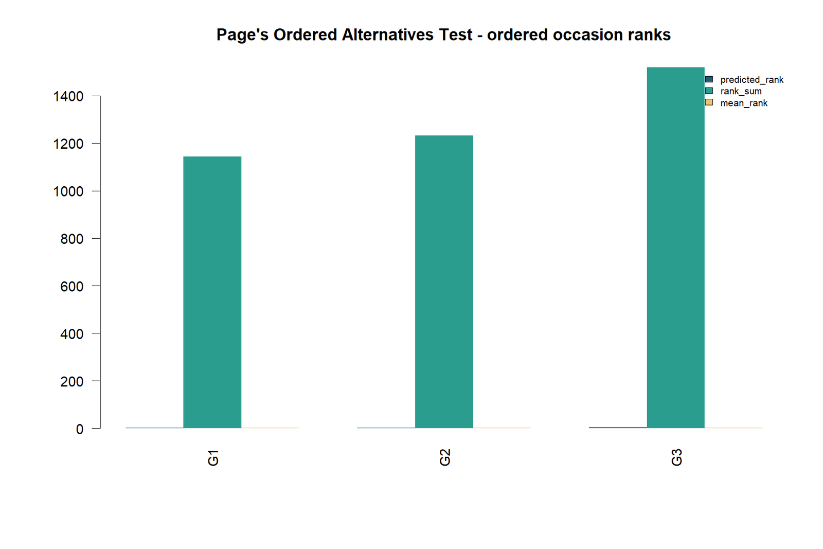
The R rank-sum bars reproduce 1,143, 1,232 and 1,519 for G1, G2 and G3. The monotonic increase is the core descriptive pattern behind L. Predicted scores and mean ranks are present but appear small because the panel uses a scale suitable for rank sums.
R chart 3: student ordered ranks
The frequency pattern matches Python: G1 most often receives the lowest rank. Agreement in the five possible average-rank categories is an important tie-handling check. If one program used minimum ranks while another used average ranks, these frequencies and the final L statistic would disagree.
R chart 4: Page standardization
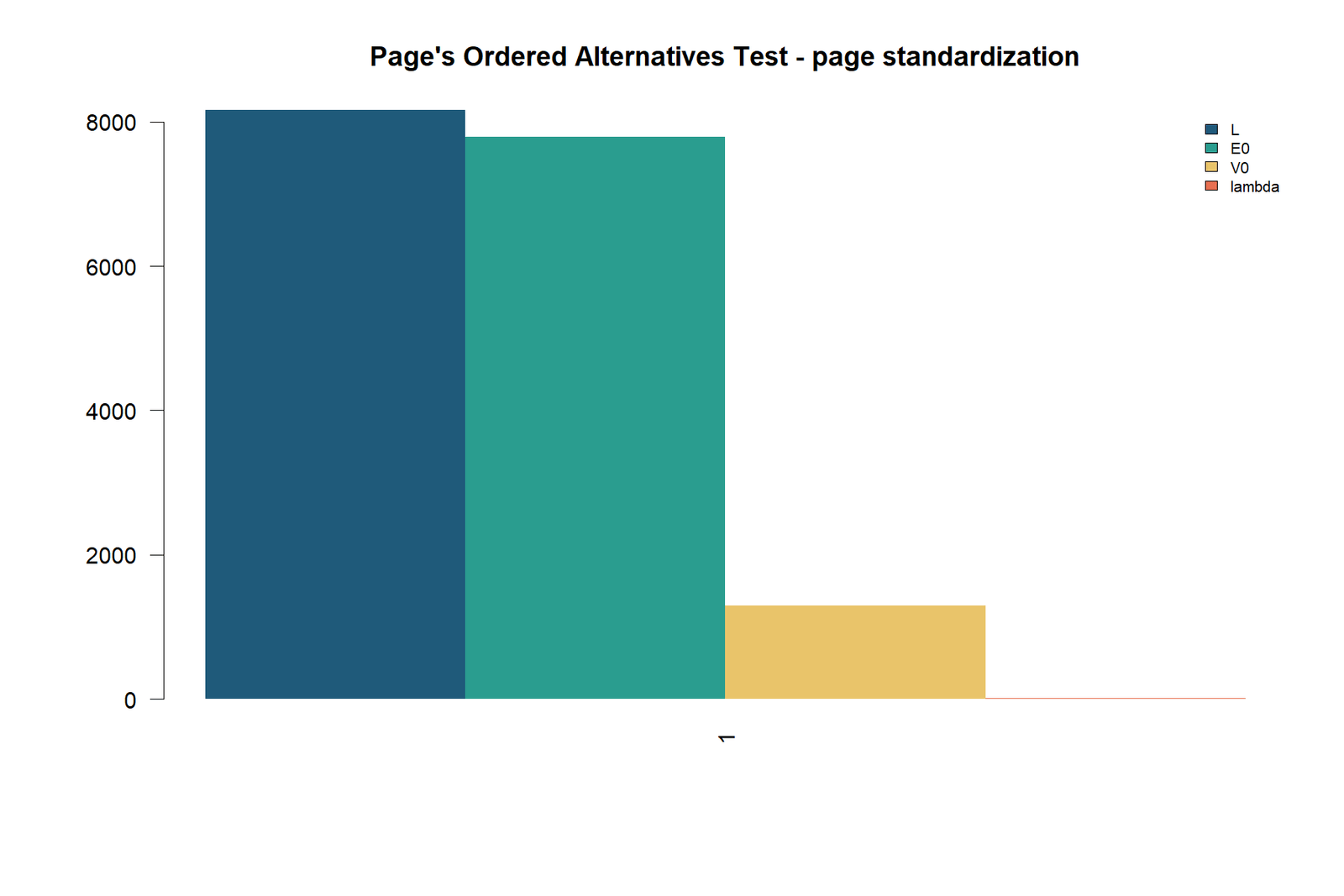
This diagnostic displays the observed L = 8,164 beside E₀ = 7,788 and V₀ = 1,298. The small fourth bar represents the standardized quantity on a much smaller scale. The meaningful calculation is the 376-point excess divided by √1,298, producing z = 10.436.
R chart 5: verified results
The horizontal result summary again confirms L, p, n and k. The Python and R reports agree to numerical precision: L is exactly 8,164 and the one-sided p-value differs only in the final floating-point digits. This agreement supports the reproducibility of the supplied workbook calculation.
How to run Page’s trend test in Python
Rank rows with average ties, calculate L, and use the upper normal tail.
Python does not require a dedicated black-box function to reproduce Page’s trend test. SciPy supplies the ranking and probability functions, while NumPy makes the calculation auditable.
import numpy as np
import pandas as pd
from scipy.stats import rankdata, norm, friedmanchisquare# One complete row per student and one column per ordered occasion.
df = pd.read_csv("dataset.csv")
wide = df[["G1", "G2", "G3"]].dropna().astype(float)
# Average ranks are assigned within each student block.
ranks = np.apply_along_axis(rankdata, 1, wide.to_numpy(), method="average")
n, k = ranks.shape
rank_sums = ranks.sum(axis=0)
mean_ranks = ranks.mean(axis=0)
ordered_scores = np.arange(1, k + 1)
# Page L for the prespecified order G1 < G2 < G3.
L = float(np.dot(ordered_scores, rank_sums))
E0 = n * k * (k + 1) ** 2 / 4
V0 = n * k ** 2 * (k + 1) ** 2 * (k - 1) / 144
z = (L - E0) / np.sqrt(V0)
p_one_sided = norm.sf(z)
# Supporting unordered omnibus test and concordance effect size.
fr = friedmanchisquare(*(wide[c] for c in wide.columns))
kendall_w = fr.statistic / (n * (k - 1))
print("n blocks:", n)
print("rank sums:", dict(zip(wide.columns, rank_sums)))
print("mean ranks:", dict(zip(wide.columns, mean_ranks)))
print("Page L:", L)
print("E0:", E0)
print("V0:", V0)
print("z:", z)
print("one-sided p:", p_one_sided)
print("Friedman chi-square:", fr.statistic)
print("Friedman p:", fr.pvalue)
print("Kendall W:", kendall_w)
Correct ranking axis
np.apply_along_axis(rankdata, 1, ...) ranks across each student’s occasions. Using axis 0 would rank students within each grade column and calculate a completely different statistic.
Upper-tail probability
norm.sf(z) is preferable to 1 - norm.cdf(z) for an extreme positive z because the survival function retains better numerical precision in the far tail.
Validation outputs
Print n, k, rank sums, mean ranks, L, E₀, V₀ and z. A single p-value is not enough to detect an incorrect column order or ranking direction.
How to run Page’s trend test in R
Use an ordered factor in coin or reproduce the formula directly.
R offers both a high-level conditional inference framework and a transparent manual route for Page’s trend test. Using both is a strong reproducibility practice.
# install.packages(c("coin", "tidyr", "dplyr"))
library(coin)
library(tidyr)
library(dplyr)dat <- read.csv("dataset.csv")
wide <- na.omit(dat[c("G1", "G2", "G3")])
wide$student <- seq_len(nrow(wide))
long <- pivot_longer(
wide,
cols = c(G1, G2, G3),
names_to = "occasion",
values_to = "grade"
)
long$occasion <- ordered(long$occasion, levels = c("G1", "G2", "G3"))
long$student <- factor(long$student)
# With an ordered condition factor and a directional alternative,
# coin's Friedman extension is Page's ordered-alternatives test.
page_result <- friedman_test(
grade ~ occasion | student,
data = long,
alternative = "greater",
distribution = "asymptotic"
)
print(page_result)
# Manual audit matching the supplied workbook and reports.
ranks <- t(apply(wide[c("G1", "G2", "G3")], 1, rank,
ties.method = "average"))
n <- nrow(ranks)
k <- ncol(ranks)
rank_sums <- colSums(ranks)
L <- sum(seq_len(k) * rank_sums)
E0 <- n * k * (k + 1)^2 / 4
V0 <- n * k^2 * (k + 1)^2 * (k - 1) / 144
z <- (L - E0) / sqrt(V0)
p <- pnorm(z, lower.tail = FALSE)
print(rank_sums)
print(colMeans(ranks))
print(c(L = L, E0 = E0, V0 = V0, z = z, p = p))
# Optional conditional Monte Carlo sensitivity analysis:
# page_mc <- friedman_test(
# grade ~ occasion | student, data = long,
# alternative = "greater",
# distribution = approximate(nresample = 99999)
# )
Why the factor must be ordered
In coin::friedman_test(), an ordered condition factor with scores 1, 2 and 3 turns the Friedman framework into the Page linear-rank extension. A nominal factor instead targets an unordered omnibus difference. Explicitly set the levels to G1, G2 and G3 so alphabetical or accidental ordering cannot alter the hypothesis.
Asymptotic versus approximate
The supplied report uses an asymptotic calculation. For a sensitivity analysis that conditions on the observed block structure, distribution = approximate(nresample = ...) performs Monte Carlo resampling. With an extremely strong result, ordinary Monte Carlo cannot estimate a probability as small as 10⁻²⁶, but it can still confirm that the observed statistic lies far in the upper tail.
PageTest() or page.trend.test() exist in other R packages. Their input orientation, small-sample tables and tie handling may differ. Document the package, version, matrix orientation and inference method rather than reporting only “R was used.”Page’s trend test in SPSS
SPSS supplies supporting repeated-measures tests, while the Page statistic requires a transparent custom calculation or integration.
The standard SPSS NPAR TESTS command includes Friedman, Kendall, sign and Wilcoxon procedures but no dedicated PAGE subcommand. A correct Page’s trend test workflow therefore calculates within-row ranks and L explicitly, or calls R/Python integration.
* G1, G2 and G3 must be one complete row per student.
* SPSS NPAR TESTS does not have a dedicated PAGE subcommand,
* so compute average within-row ranks explicitly for three occasions.COMPUTE rG1 = 1 + (G2 < G1) + (G3 < G1)
+ .5*((G2 = G1) + (G3 = G1)).
COMPUTE rG2 = 1 + (G1 < G2) + (G3 < G2)
+ .5*((G1 = G2) + (G3 = G2)).
COMPUTE rG3 = 1 + (G1 < G3) + (G2 < G3)
+ .5*((G1 = G3) + (G2 = G3)).
COMPUTE row_rank_check = rG1 + rG2 + rG3.
EXECUTE.
* Save the case-level file before aggregation if needed.
DATASET DECLARE PageSummary.
AGGREGATE
/OUTFILE=PageSummary
/BREAK=
/n_blocks=N
/R_G1=SUM(rG1)
/R_G2=SUM(rG2)
/R_G3=SUM(rG3).
DATASET ACTIVATE PageSummary.
COMPUTE k_occasions = 3.
COMPUTE page_L = 1*R_G1 + 2*R_G2 + 3*R_G3.
COMPUTE page_E0 = n_blocks*k_occasions*(k_occasions+1)**2/4.
COMPUTE page_V0 = n_blocks*k_occasions**2*(k_occasions+1)**2
*(k_occasions-1)/144.
COMPUTE page_z = (page_L-page_E0)/SQRT(page_V0).
COMPUTE page_p_one_sided = CDF.NORMAL(-page_z,0,1).
FORMATS R_G1 R_G2 R_G3 page_L page_E0 page_V0 (F12.3)
page_z (F12.6) page_p_one_sided (E16.8).
LIST.
* Supporting analyses on the original wide dataset:
* NPAR TESTS /FRIEDMAN=G1 G2 G3 /STATISTICS=DESCRIPTIVES QUARTILES.
* NPAR TESTS /SIGN=G1 G2 WITH G2 G3 (PAIRED).
* NPAR TESTS /WILCOXON=G1 G2 WITH G2 G3 (PAIRED).
What the supplied SPSS PDF confirms
The output verifies 649 rows, descriptive statistics, mean ranks of 1.76, 1.90 and 2.34, and a significant Friedman test, χ²(2) = 167.328, p < .001. It also reports adjacent sign and Wilcoxon comparisons. G2 exceeded G1 for 273 students versus 187 decreases, and G3 exceeded G2 for 290 students versus 72 decreases.
These outputs support the directional pattern, but Friedman, sign and Wilcoxon are not Page’s trend test. The PDF correctly echoes the independently verified Page result after the native supporting procedures.
Warnings in the PDF
The SPSS report contains a value-label warning and a 60-character subtitle truncation warning. Neither warning changes G1, G2, G3, the rank calculations or the final statistical conclusion. Future syntax should shorten the subtitle and correct the value-label statement so the public transcript is cleaner.
The manual rank formulas shown above are specific to three occasions. For more conditions, R/Python integration or a generalized SPSS matrix/Python extension is safer than writing many pairwise logical comparisons by hand.
Page’s trend test in Excel
The supplied workbook separates source values, working ranks, calculations, diagnostics and final reporting.
A formula-driven Excel implementation makes Page’s trend test easy to audit because every rank and intermediate term remains visible.
Assume G1:G3 occupy A5:C653.D5: =RANK.AVG(A5,$A5:$C5,1)
E5: =RANK.AVG(B5,$A5:$C5,1)
F5: =RANK.AVG(C5,$A5:$C5,1)
Copy D5:F5 through row 653.
Rank sum G1: =SUM(D5:D653)
Rank sum G2: =SUM(E5:E653)
Rank sum G3: =SUM(F5:F653)
n blocks: =COUNT(A5:A653)
k occasions: =3
Page L: =1*RankSum_G1+2*RankSum_G2+3*RankSum_G3
E0: =n*k*(k+1)^2/4
V0: =n*k^2*(k+1)^2*(k-1)/144
z: =(Page_L-E0)/SQRT(V0)
One-sided p: =NORM.S.DIST(-z,TRUE)
Rank-total audit: =SUM(RankSum_G1:RankSum_G3)
Expected total: =n*k*(k+1)/2
Decision: =IF(p<0.05,"Reject H0","Do not reject H0")
Guide sheet
Documents the complete-block design, G1-G2-G3 order, null hypothesis, formula, 649 source rows and α = .05. This prevents the workbook from becoming an unexplained collection of formulas.
Data_Input sheet
Contains only the unchanged three-grade matrix. Source values are separated from derived ranks so a reviewer can confirm that the analysis did not overwrite or silently transform raw data.
Working sheet
Calculates average ranks for each row, range-based diagnostic values and tie terms. Every row can be traced from raw grades to its ranks and weighted contribution.
Calculations sheet
Reports rank sums 1,143, 1,232 and 1,519; Page L = 8,164; E₀ = 7,788; V₀ = 1,298; z = 10.4364; and supporting Friedman, Kendall W and Quade values.
Diagnostics sheet
Records that each student is a complete block, within-row ties receive average ranks, and the method identity is the ordered Page statistic.
Reporting sheet
Compares workbook output with independently verified values. The L statistic and block count have zero absolute difference. The displayed workbook p may round to zero, so the verified reference retains 8.4556 × 10⁻²⁶.
NORM.S.DIST(-z,TRUE). Subtracting a CDF extremely close to 1 can lose precision. Format the cell in scientific notation to prevent a tiny nonzero p-value from appearing as 0.000.Page’s trend test assumptions and diagnostics
The critical requirements concern design, ordering and independence rather than normality.
Like every rank procedure, Page’s trend test is distribution-free only within a defined design. It does not remove the need to justify blocks, measurement, missing-data rules or the direction of the alternative.
Core assumptions
Not required
However, markedly different measurement scales or ceiling effects can complicate interpretation. Rank robustness does not repair a poorly defined repeated-measures design.
Check row completeness
Confirm that exactly 649 rows enter every calculation. Different listwise deletion across programs is a common source of disagreement.
Check rank totals
Each row must total 6 and all rank sums must total 3,894. These identities quickly expose wrong-axis ranking.
Inspect ties
Eighty-nine students have all three grades equal, and many more have one tied pair. Average-rank consistency is essential.
Inspect order stability
Means, medians and rank sums all rise, but the scientific order should still come from design rather than these observed summaries.
Report effect context
Kendall’s W = 0.1289 is modest. An enormous z does not imply an enormous educational effect.
Consider resampling
A blockwise Monte Carlo test can preserve observed ties and provide a sensitivity check when conventional asymptotic formulas are questioned.
Page’s trend test compared with related methods
Design and hypothesis determine the correct nonparametric procedure.
The name “trend test” covers several unrelated methods. Comparing Page’s trend test with nearby procedures prevents common design errors.
| Method | Data structure | Main hypothesis | Direction | When it fits |
|---|---|---|---|---|
| Page’s trend test | Three or more related conditions / complete blocks | Prespecified monotonic rank order | Usually one-sided | Ordered repeated measures |
| Friedman test | Three or more related conditions | Any difference among condition rank distributions | Omnibus | No planned order or nonmonotonic alternatives matter |
| Jonckheere-Terpstra | Three or more independent ordered groups | Ordered stochastic trend | One-sided | Different participants in each ordered group |
| Quade test | Related complete blocks | Condition differences weighted by block range | Omnibus | Blocks differ meaningfully in informativeness |
| Kendall’s W | Related rankings | Strength of concordance | Effect-size style | Quantifying agreement after Friedman-like ranking |
| Nemenyi test | Related conditions after Friedman | Which mean-rank pairs differ | All pairs | Post hoc localization, not a trend statistic |
| Repeated-measures ANOVA | Related numeric outcomes | Mean differences under parametric model | Omnibus/contrasts | Model assumptions and scale support mean inference |
| Mixed-effects model | Longitudinal or clustered outcomes | Model-based time, treatment and interaction effects | Flexible | Missing observations, covariates or complex trajectories |
Page’s trend test vs Friedman test
Friedman asks whether any condition differs; Page asks whether the differences align with a specified linear order. In this dataset, both are significant. That agreement is reassuring, but the tests are not duplicates. A U-shaped sequence could be strongly significant by Friedman and weak under an increasing Page alternative.
Page’s trend test vs Jonckheere-Terpstra
Both target ordered alternatives and are rank based. The dependence structure separates them. Page ranks conditions inside each shared block. Jonckheere-Terpstra compares observations across independent ordered groups. Substituting one for the other changes both the statistic and its reference distribution.
Other useful comparisons include the Mann-Whitney U test for two independent groups, Kruskal-Wallis for several independent groups, Nemenyi post hoc comparisons, Dunn’s test, Conover’s test, the two-sample Kolmogorov-Smirnov test, Ansari-Bradley and the Moses test of extreme reactions. These answer different questions about location, distribution or dispersion.
How to interpret and report Page’s trend test
Combine the directional statistic with descriptive change, effect context and design limitations.
A complete Page’s trend test report identifies the planned order, number of blocks, condition summaries, L statistic, inference method, one-sided p-value and substantive conclusion.
APA-style result
A Page test for ordered alternatives evaluated the prespecified increasing grade sequence G1 < G2 < G3 for 649 students. Mean ranks increased from 1.761 at G1 to 1.898 at G2 and 2.341 at G3. The ordered trend was statistically significant, L = 8,164, z = 10.44, one-sided p < .001. Raw grade means were 11.40, 11.57 and 11.91, respectively. The supporting Friedman test was also significant, χ²(2) = 167.33, p < .001, with Kendall’s W = .129.
Plain-language interpretation
Students tended to receive higher grades at later occasions, and the ordering was much stronger than expected if the three grade labels were unrelated to within-student rank. The improvement was not universal: 398 students followed a nondecreasing sequence and 251 did not. The average raw increase from G1 to G3 was about 0.51 grade points.
| Reporting element | Recommended wording | Avoid |
|---|---|---|
| Order | “The G1 < G2 < G3 order was prespecified.” | “The best order was discovered to be…” |
| Decision | “Evidence supported an increasing trend.” | “All students improved.” |
| Probability | “One-sided p = 8.46 × 10⁻²⁶” or “p < .001.” | “There is a 99.9% probability the alternative is true.” |
| Magnitude | Report raw means/medians and Kendall’s W. | Treat z or L as a universal effect size. |
| Causality | Describe an ordered association unless design supports causation. | Claim that the occasion caused improvement from a rank test alone. |
Page’s trend test downloads and reproducible files
Use the reports and workbook to reproduce every result shown in this guide.
The Page’s trend test download package includes independent Python and R reports, SPSS supporting output, and a formula-driven Excel workbook.
R PDF reportIndependent R calculation and five supporting charts.Open R report →
SPSS PDF outputDescriptives, Friedman, sign, Wilcoxon and embedded verified Page result.Open SPSS output →
Excel worked analysisRaw data, row ranks, formula calculations, diagnostics and reporting.Download workbook →
Reproduction checklist
Software agreement
Python and R reproduce the same Page L and p-value to floating-point precision. Excel reproduces L exactly and stores the verified probability reference. SPSS confirms the descriptive and repeated-measures pattern, while the Page statistic is supplied through the custom formula or integration rather than a native PAGE menu command.
Page’s trend test FAQs
Answers to common questions about design, formulas, software, ties and interpretation.
What is Page’s trend test?
Page’s trend test is a nonparametric test for a prespecified monotonic order across three or more related conditions or complete-block treatments. It ranks conditions within each block and weights condition rank sums by ordered scores.
Is Page’s trend test the same as the Friedman test?
No. Page’s trend test and Friedman answer different questions. Friedman detects any repeated-condition difference and does not require a directional order. Page’s trend test focuses on one planned monotonic sequence and is usually one-sided.
What is the Page L statistic?
In Page’s trend test, Page L is the weighted sum of condition rank totals: L = ΣjRj. High ranks appearing in conditions with high order scores make L large. In the worked example, L = 8,164.
What are the assumptions of Page’s trend test?
The main assumptions of Page’s trend test are related observations within blocks, independent blocks, at least ordinal outcomes, comparable measurement, a prespecified order and consistent handling of ties and missing values. Normality is not required.
How are ties handled?
In Page’s trend test, tied values within a row receive average ranks. For example, 11, 11 and 13 receive ranks 1.5, 1.5 and 3. Conditional permutation or Monte Carlo inference can be used as a sensitivity analysis when ties are extensive.
Is Page’s trend test one-sided?
Page’s trend test is usually one-sided because it tests a specified increasing or decreasing order. The direction must be chosen before inspecting outcomes. Reverse the condition order for a planned decreasing alternative.
Can I choose the order after looking at means?
Not for a confirmatory p-value. Selecting the order that maximizes L uses the data twice and makes the ordinary one-sided reference anti-conservative. Treat that search as exploratory and confirm the order in new data.
How do I run Page’s trend test in Python?
Rank each row with scipy.stats.rankdata(..., method="average"), sum ranks by condition, calculate L, E₀ and V₀, standardize to z and use scipy.stats.norm.sf(z) for the increasing upper tail.
How do I run Page’s trend test in R?
Use coin::friedman_test() with an ordered condition factor, a block identifier and alternative="greater". You can also calculate the Page formula manually or use a dedicated Page-test package after verifying matrix orientation and tie rules.
Does SPSS have a native Page test menu?
The standard SPSS NPAR TESTS command does not list a dedicated PAGE subcommand. Use custom within-row rank formulas, R/Python integration, or an audited workbook. SPSS Friedman and paired tests are supporting analyses, not substitutes with the same name.
Can Excel calculate Page’s trend test?
Yes. RANK.AVG calculates within-row ranks, ordinary formulas calculate rank sums and L, and NORM.S.DIST(-z,TRUE) calculates the one-sided asymptotic p-value. The supplied workbook includes all intermediate sheets.
What did Page’s trend test find in this example?
The test found strong evidence for G1 < G2 < G3: L = 8,164, z = 10.436 and one-sided p = 8.4556 × 10⁻²⁶. Mean ranks increased from 1.761 to 1.898 to 2.341.
Does the significant result mean every student improved?
No. A population-level ordered tendency can be significant even when many individual rows are flat or move in another direction. Here, 398 students were nondecreasing and 251 had another pattern.
What effect size should accompany Page’s trend test?
There is no single universally reported Page-specific effect size. Report original summaries, rank means and an overall repeated-rank effect such as Kendall’s W when useful. In this example W = 0.1289.
Why is the p-value so much smaller than the raw grade changes look?
The sample contains 649 repeated blocks, so even a modest but consistent ordering produces a large standardized statistic. Statistical evidence and practical magnitude are different; report both.
What should I do with missing repeated observations?
A simple Page’s trend test calculation requires complete blocks. State the deletion rule. When missingness is meaningful or many rows are incomplete, consider a mixed-effects or other longitudinal model that can use partial records under explicit assumptions.
What is the difference between Page’s trend test and Jonckheere-Terpstra?
Page’s trend test is for related conditions observed in the same blocks. Jonckheere-Terpstra is for independent groups arranged in an expected order. Their rankings and null distributions are different.
Do I need post hoc tests after Page’s trend test?
Page’s trend test answers the global ordered question. If the research also requires pairwise localization, use planned contrasts or an appropriate multiplicity-controlled repeated-measures post hoc procedure such as Nemenyi, while keeping that secondary question distinct.