
Nemenyi Test: Formula, Interpretation, Python, R, SPSS and Excel Guide
The Nemenyi test is an all-pairs rank comparison procedure most commonly used after a significant Friedman test. This complete guide explains the Nemenyi post hoc test formula, assumptions, critical difference, studentized-range decision rule, a 649-student worked example, interpretation, and reproducible workflows in Python, R, SPSS and Excel.
Repeated measures
Mean ranks
Familywise inference
Python + R + SPSS + Excel
All three grade occasions differed in mean rank.
For 649 students measured at G1, G2 and G3, the omnibus Friedman test was significant, χ²(2) = 167.328, p < .001. The Nemenyi test then compared every pair of mean ranks using a standard error of 0.055513, a critical q value of 2.343701, and a critical difference of 0.130105. G1 versus G2 differed by 0.137134, G1 versus G3 by 0.579353, and G2 versus G3 by 0.442219. Every absolute difference exceeded the critical difference, so all three pairwise null hypotheses were rejected at α = .05.
What does the Nemenyi test measure?
An all-pairs comparison of mean ranks after a repeated-measures omnibus test.
The Nemenyi test identifies which conditions differ after an omnibus rank test has shown that at least one condition is not equivalent. In the post-Friedman setting, the same blocks or participants are observed under several conditions, each row is ranked internally, and the Nemenyi post hoc test compares the resulting condition mean ranks.
The statistical target
The Friedman test answers a global question: are the repeated conditions drawn from populations with the same rank location? A significant omnibus result does not reveal which occasions differ. The Nemenyi test supplies that second stage by evaluating every pair, such as G1 versus G2, G1 versus G3, and G2 versus G3.
The Nemenyi test evidence is based on the distance between two mean ranks relative to a common standard error. The studentized-range distribution sets a simultaneous threshold, so the family of pairwise decisions is evaluated more conservatively than unadjusted pairwise tests. This is why the method is described as a multiple-comparison procedure rather than three unrelated tests.
What the result means
A significant Nemenyi test pair indicates that the two conditions have different average positions within the blockwise rankings. A positive or negative difference supplies direction according to the subtraction order, while the condition mean ranks provide the clearest substantive ordering.
The Nemenyi procedure does not directly compare arithmetic means, standard deviations or raw-score medians. If the scientific question concerns paired raw differences, a sign test or a multiplicity-adjusted Wilcoxon signed-rank analysis may answer a different and sometimes more direct question. If the design contains independent groups instead of repeated conditions, use the appropriate post-Kruskal-Wallis method.
When should you use the Nemenyi test?
Start with the design and omnibus result, not merely with non-normal data.
Use the Nemenyi test when there are at least three related conditions, the Friedman null hypothesis has been rejected, and the research goal is to locate pairwise differences while accounting for the full comparison family.
Confirm repeated data
Each participant or block contributes one usable value to every condition being compared.
Run Friedman first
Establish an omnibus difference before interpreting post hoc pairs.
Rank within blocks
Assign average ranks when repeated values are tied inside a row.
Compare all pairs
Calculate mean-rank differences and studentized-range q statistics.
Report direction
Use mean ranks and original descriptive statistics to explain the pattern.
Good research situations
Choose another method when
Do not select the Nemenyi post hoc test for two conditions only; a direct paired test is sufficient. Do not use the blocked formula for independent groups. Do not use it when many blocks are incomplete without first choosing a method designed for missing repeated observations. Do not treat it as a substitute for a model when covariates, interactions, clusters or longitudinal trajectories are central.
For parametric repeated-measures questions, consider repeated-measures ANOVA or a mixed-effects model. For several independent groups, compare Dunn’s test, Conover’s test and the independent-samples Nemenyi variant rather than importing the Friedman formula.
Why use a Nemenyi post hoc test?
The Nemenyi test is useful because the Friedman statistic is global. A significant χ² value says that the repeated distributions are not all equivalent, but it leaves the location of the difference unresolved. The post hoc Nemenyi procedure converts the same blockwise ranks into simultaneous pairwise decisions. It is therefore most defensible when the omnibus analysis, post hoc analysis and interpretation are planned as one coherent workflow.
How the Nemenyi test works
The entire Nemenyi test method can be audited from row-level ranks to the final critical-difference decision.
The Nemenyi test begins with the same rank structure used by Friedman’s test. Each complete block is ranked across conditions, the ranks are averaged by condition, and pairwise mean-rank distances are compared against a studentized-range threshold.
Step-by-step logic
- Arrange data in wide format with one row per block and one column per condition.
- Rank the conditions inside each row from lowest to highest; ties receive their average rank.
- Average each condition’s ranks across all blocks.
- Compute the common standard error from the number of conditions and blocks.
- Calculate the absolute difference for every pair of condition mean ranks.
- Convert each difference to the Nemenyi q scale.
- Compare q with the critical q value, or compare the raw mean-rank difference with the critical difference.
- Use the studentized-range distribution for multiplicity-aware p-values.
Two equivalent decision routes
The Nemenyi test q route rejects a pair when its Nemenyi q statistic is larger than the critical q value. The critical-difference route rejects when the absolute mean-rank difference is larger than the critical difference. Because the critical difference is simply the critical q multiplied by the standard error, both routes must produce identical decisions.
In the worked analysis, the smallest q was 2.470317 and the critical q was 2.343701. Equivalently, the smallest absolute mean-rank difference was 0.137134 and the critical difference was 0.130105. The pair is significant by both routes, though its margin is much narrower than the margins for comparisons involving G3.
Variables and data dictionary for the worked analysis
The example uses three within-student grade occasions from 649 complete records.
This Nemenyi test example treats each student as a block. G1, G2 and G3 are repeated grade occasions, not independent groups. The same 649 students appear in every column used by the post-Friedman comparison.
| Variable | Role | Scale | Observed summary | Analysis treatment |
|---|---|---|---|---|
| Student | Block / repeated unit | Identifier | 649 complete blocks | Ranks are assigned within each student |
| G1 | First grade occasion | Numeric, 0-19 observed | Mean 11.40; SD 2.745; median 11 | Mean rank 1.761171 |
| G2 | Second grade occasion | Numeric, 0-19 observed | Mean 11.57; SD 2.914; median 11 | Mean rank 1.898305 |
| G3 | Final grade occasion | Numeric, 0-19 observed | Mean 11.91; SD 3.231; median 12 | Mean rank 2.340524 |
| Within-row rank | Derived score | 1 to 3 with average ties | Three ranks per complete row | Input to Friedman and Nemenyi calculations |
Outcome meaning
The grades are ordered numerical outcomes. A higher within-student rank means that the occasion’s grade was higher relative to that student’s other two grades. The test does not assume that the distance from 10 to 11 has a normal sampling distribution.
Block meaning
Dependence inside a student is expected and is the reason for the blocked design. Independence is required across students: one student’s grade sequence should not determine another student’s sequence.
Tie meaning
When a student has equal grades on two or three occasions, average ranks preserve the total rank contribution. Ties reduce the amount of ordering information, so their frequency belongs in diagnostics.
Before any rank analysis, review descriptive statistics, frequency distributions, means and medians, and possible outliers. A post hoc rank result is clearer when the reader can connect mean-rank direction to the original measurement scale.
Nemenyi test assumptions and design conditions
Nonparametric does not mean assumption-free.
The Nemenyi test assumptions concern design validity, rankability, completeness and interpretable distributions. The Nemenyi test does not require normal raw scores or the parametric equal-variance assumption used by conventional ANOVA.
1. Related conditions
The Friedman-Nemenyi test requires repeated measurements or matched treatments. Every analyzed row represents a coherent block observed under the same set of conditions.
2. Independent blocks
Blocks should be independent of one another. Students may be dependent across G1, G2 and G3 within their own rows, but one student should not be duplicated as another independent case.
3. Ordered outcomes
Values must support meaningful ordering. Numeric grades qualify. Pure labels without an order cannot be ranked and should instead be analyzed with categorical procedures.
4. Complete comparable occasions
The classic calculation assumes all included blocks contain all k conditions. Selective missingness can change the analyzed population and may call for a longitudinal model.
5. Consistent measurement
The conditions should measure the same construct on a comparable scale. A high rank must have a similar substantive meaning across occasions.
6. Interpretable shapes
Rank tests can detect ordering differences without normality, but location language is clearest when distributions differ mainly in position rather than in radically different shapes.
Normality is not required
There is no requirement that G1, G2 and G3 follow normal distributions. Therefore a failed Shapiro-Wilk test is not, by itself, the reason to use Nemenyi. The design, outcome scale and inferential target are more important than a mechanical normality screen.
Ties require attention
Average ranks handle within-row ties computationally. Still, a dataset dominated by ties provides less discrimination among conditions. Report the tie pattern, compare original medians and consider a sensitivity analysis based on paired differences if the substantive conclusion rests on a very small margin.
Nemenyi test hypotheses and direction
Each post hoc hypothesis concerns one pair inside a family of comparisons.
For k conditions, the Nemenyi test evaluates k(k – 1)/2 pairwise null hypotheses. With three grade occasions there are three comparisons. The studentized-range threshold accounts for considering the full family rather than treating each pair in isolation.
Pairwise hypotheses
Null hypothesis, H0,ij
The population mean ranks for conditions i and j are equal. In applied language, neither condition has a systematically higher rank position than the other.
Alternative hypothesis, H1,ij
The population mean ranks for conditions i and j differ. The standard Nemenyi test procedure is two-sided; direction is interpreted from the ordered mean ranks after significance is established.
Family in this example
H0: mean ranks are equal.
H0: mean ranks are equal.
H0: mean ranks are equal.
The ordering G1 < G2 < G3 is descriptive. The inferential decisions are based on absolute differences, so the same critical threshold applies regardless of subtraction order.
Nemenyi test formula, q statistic and critical difference
The Nemenyi test formula converts mean-rank separation into a common studentized-range scale.
The Nemenyi test formula uses the absolute difference between two condition mean ranks and a standard error determined by k conditions and n complete blocks.
R̄i and R̄j are condition mean ranks, k is the number of repeated conditions, and n is the number of complete blocks. This article reports q on the scale used by the supplied workbook, where the conventional studentized-range variate is q√2.
The critical difference is the minimum absolute mean-rank distance required for significance. For k = 3, n = 649 and α = .05, qcritical = 2.343700586 and CD = 0.130105237.
Critical-value decision
Reject H0,ij when qij > qcritical. All observed q statistics exceeded 2.343701. The G1-G2 statistic exceeded it only modestly, while both comparisons involving G3 exceeded it by a large amount.
Critical-difference decision
Reject H0,ij when |R̄i − R̄j| > CD. The smallest observed difference, 0.137134, exceeded 0.130105 by 0.007029. This narrow margin makes exact preprocessing, tie ranking and complete-case selection especially important for the G1-G2 conclusion.
Nemenyi test worked example: G1, G2 and G3 grades
A complete calculation from omnibus evidence to all-pairs interpretation.
The worked Nemenyi test example uses 649 complete student records. Each row contains three grade occasions. The analysis asks whether the average within-student rank is equal across G1, G2 and G3.
Step 1: omnibus Friedman result
The Friedman statistic was χ²(2) = 167.328 with p < .001. Therefore the null hypothesis that all three repeated grade occasions have the same rank distribution was rejected. The corresponding Kendall’s W was 0.128912, indicating that the repeated occasions account for a modest but clearly detectable ordering pattern across a large sample.
Because the omnibus result is significant, pairwise post hoc analysis is warranted. The large sample makes even a relatively small mean-rank difference potentially detectable, so statistical significance should be interpreted alongside the original grade summaries and rank separation.
Verified Nemenyi conclusion
Every pair exceeded the α = .05 critical difference.
G1 < G2 < G3 in mean rank
| Comparison | Signed mean-rank difference | Absolute difference | Nemenyi q | Adjusted p | Decision |
|---|---|---|---|---|---|
| G1 vs G2 | −0.137134 | 0.137134 | 2.470317 | 0.035991 | Reject H0 |
| G1 vs G3 | −0.579353 | 0.579353 | 10.436395 | Numerically underflowed to 0 in Python | Reject H0 |
| G2 vs G3 | −0.442219 | 0.442219 | 7.966078 | 4.88498 × 10⁻¹⁵ | Reject H0 |
Nemenyi test results and Python chart findings
Five charts summarize the calculation from global constants to pairwise decisions.
The Python charts make the Nemenyi test auditable. They show the standard error and critical threshold, the ordering of mean ranks, each pairwise q statistic, the critical-difference decisions, and a compact verification summary.
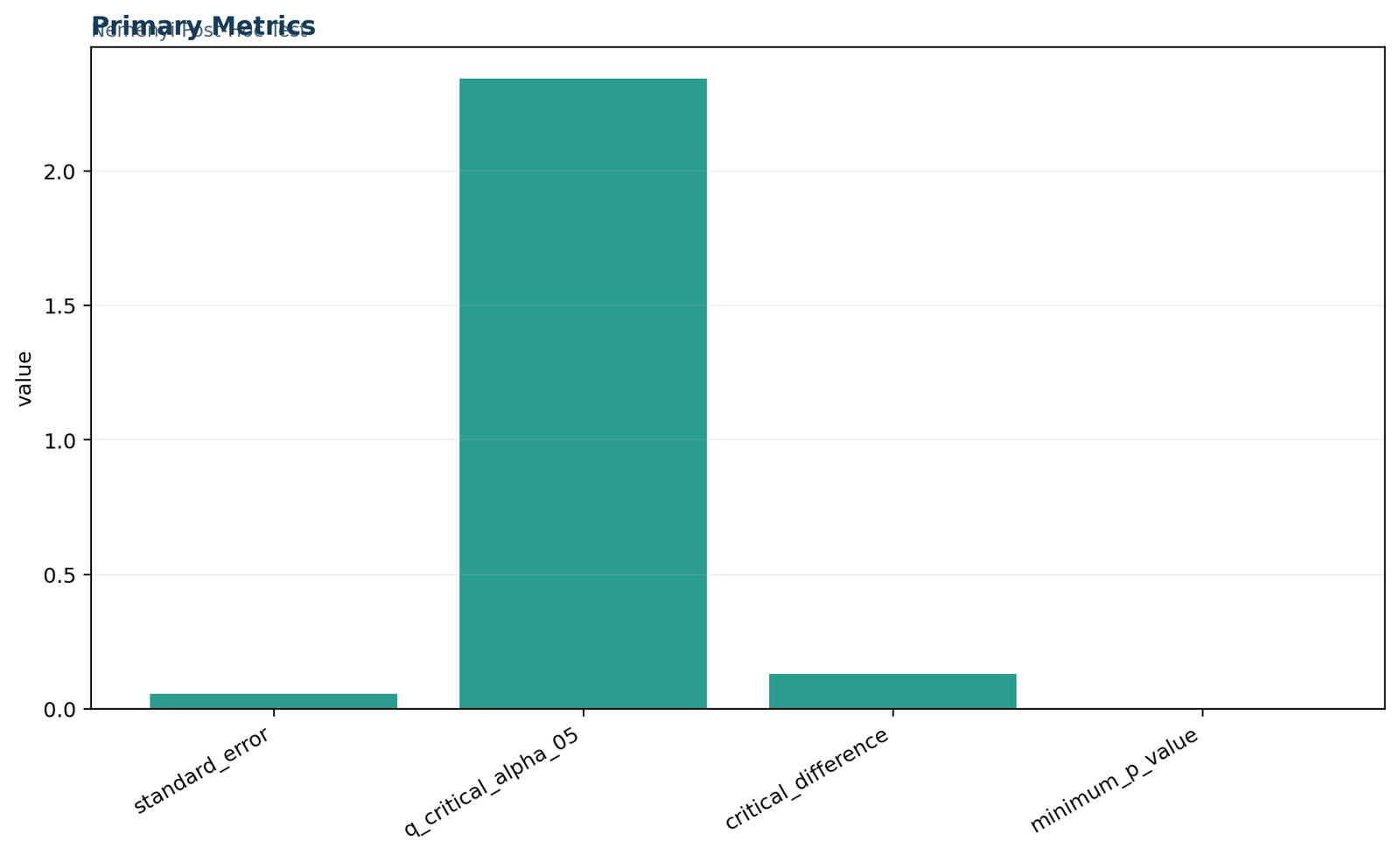
Python chart 1: primary metrics
The q critical value dominates the common scale because it is 2.343701, while the standard error is 0.055513 and the critical difference is 0.130105. The minimum p-value appears as zero because the smallest studentized-range tail probability underflows numerically.
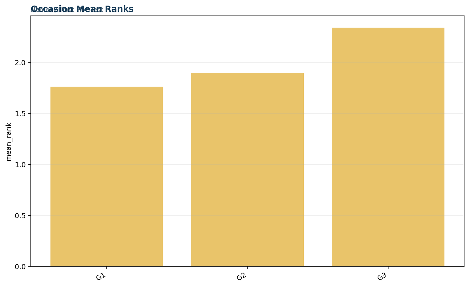
Python chart 2: occasion mean ranks
The bars increase from G1 (1.761171) to G2 (1.898305) to G3 (2.340524). This ordered pattern provides direction for the significant pairwise findings and aligns with the raw means of 11.40, 11.57 and 11.91.
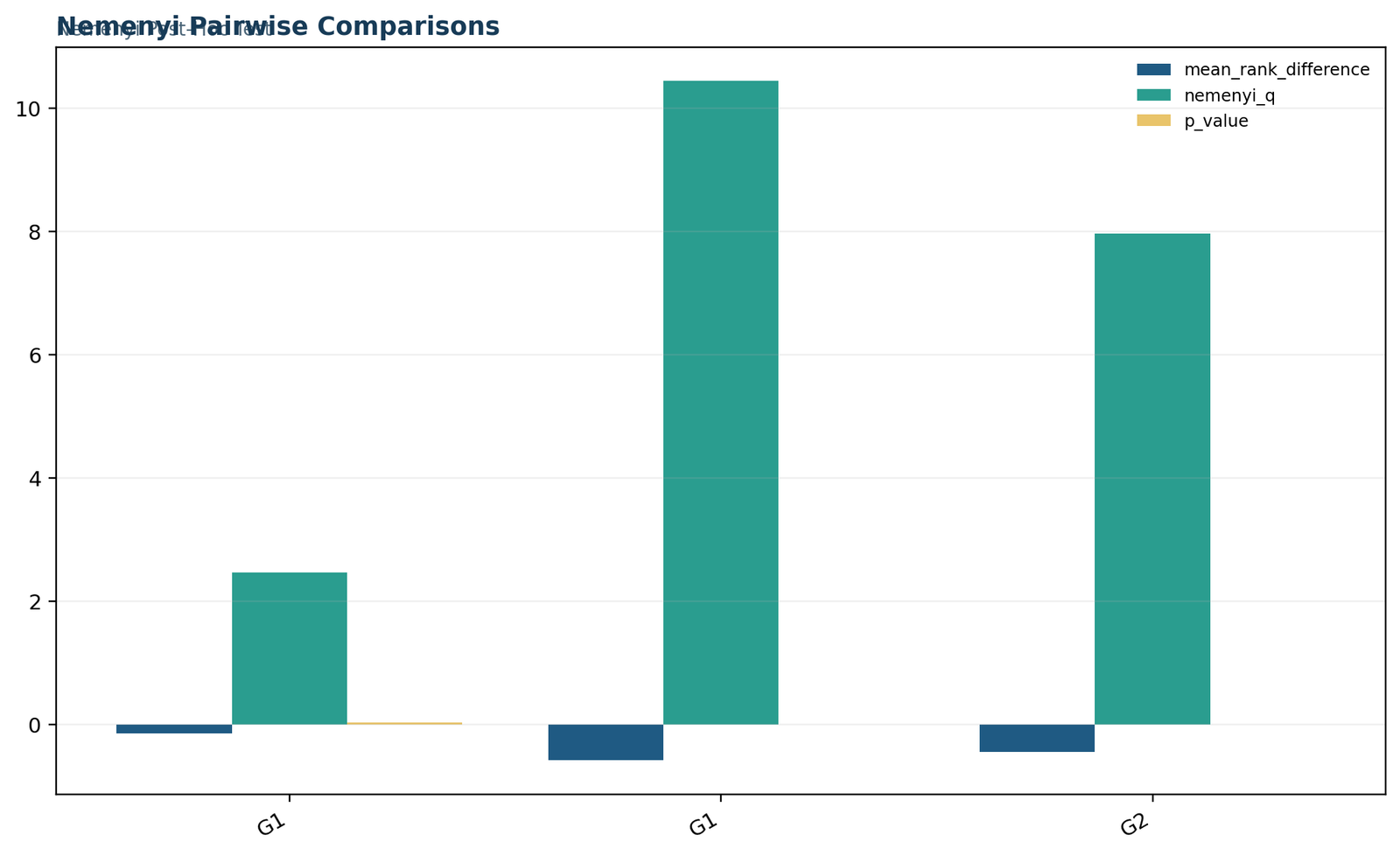
Python chart 3: pairwise comparisons
The Nemenyi q values are 2.470317, 10.436395 and 7.966078. The much larger bars for comparisons involving G3 show that the main rank separation occurs between the final grade and the two earlier occasions.
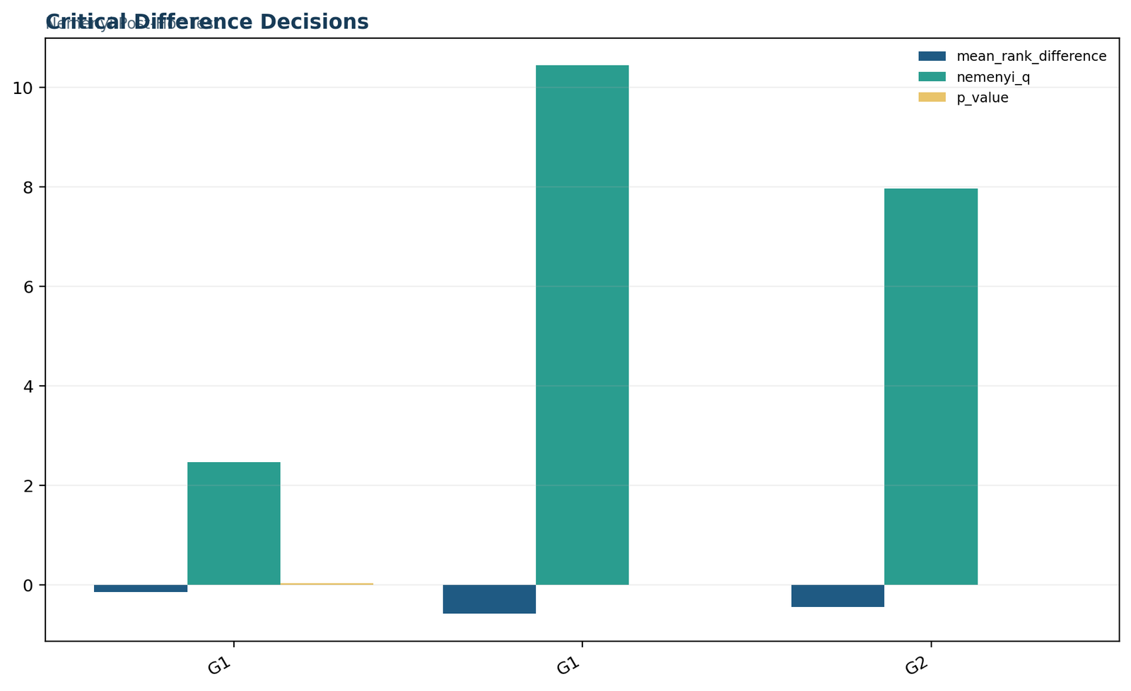
Python chart 4: critical-difference decisions
Every pair is marked significant because each absolute mean-rank difference exceeds 0.130105. The G1-G2 difference is only slightly above the line, so it should be described as statistically significant but much smaller than either G3 comparison.
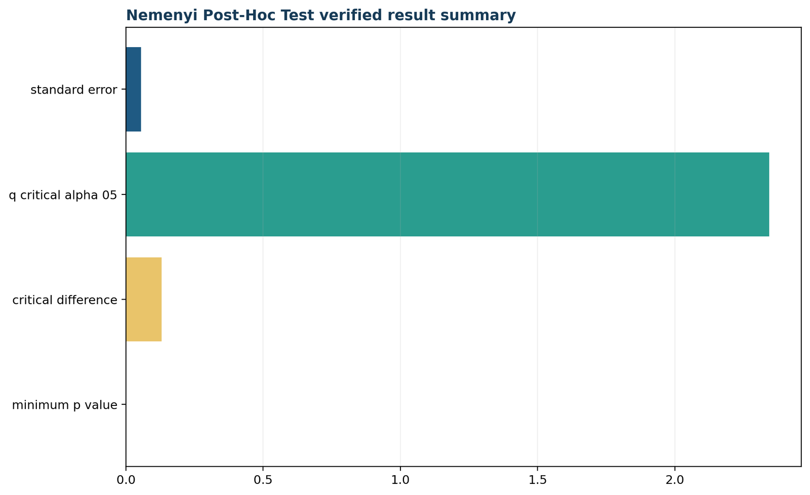
Python chart 5: verified result summary
The summary repeats the four constants independently checked against the workbook. Agreement between the calculated and reference values supports the computational reproducibility of the Nemenyi test result.
Nemenyi test in Python
A transparent implementation using SciPy’s studentized-range distribution.
A reproducible Nemenyi test Python workflow should rank each row, verify the Friedman omnibus result, calculate mean ranks and use a studentized-range distribution for simultaneous pairwise inference.
import itertools
import numpy as np
import pandas as pd
from scipy.stats import rankdata, friedmanchisquare, studentized_range# One row per student; G1, G2, and G3 are repeated occasions.
df = pd.read_csv("dataset.csv")
wide = df[["G1", "G2", "G3"]].dropna().astype(float)
# Average ranks are assigned within each student/block.
ranks = np.apply_along_axis(rankdata, 1, wide.to_numpy(), method="average")
labels = list(wide.columns)
n, k = ranks.shape
mean_ranks = ranks.mean(axis=0)
# Omnibus Friedman test should precede post-hoc interpretation.
fr_stat, fr_p = friedmanchisquare(*(wide[c] for c in labels))
alpha = 0.05
standard_error = np.sqrt(k * (k + 1) / (6 * n))
q_critical = studentized_range.ppf(1 - alpha, k, np.inf) / np.sqrt(2)
critical_difference = q_critical * standard_error
rows = []
for i, j in itertools.combinations(range(k), 2):
difference = mean_ranks[i] - mean_ranks[j]
q_value = abs(difference) / standard_error
# The studentized-range object uses the conventional range scale,
# so the workbook's q statistic is multiplied by sqrt(2).
p_value = studentized_range.sf(q_value * np.sqrt(2), k, np.inf)
rows.append({
"occasion_1": labels[i],
"occasion_2": labels[j],
"mean_rank_difference": difference,
"nemenyi_q": q_value,
"p_value": p_value,
"significant": abs(difference) > critical_difference,
})
results = pd.DataFrame(rows)
print("Friedman chi-square:", fr_stat)
print("Friedman p-value:", fr_p)
print("Mean ranks:", dict(zip(labels, mean_ranks)))
print("Standard error:", standard_error)
print("Critical q:", q_critical)
print("Critical difference:", critical_difference)
print(results.to_string(index=False))
Why the √2 conversion appears
The workbook defines q as the mean-rank difference divided by √[k(k + 1)/(6n)]. SciPy’s studentized-range distribution is conventionally parameterized for a range statistic whose equivalent value is q√2. Dividing the critical studentized-range quantile by √2 and multiplying the observed q by √2 for the survival probability keeps both sides on compatible scales.
Python result checks
The code should reproduce mean ranks 1.761171, 1.898305 and 2.340524; standard error 0.055512738; critical q 2.343700586; and critical difference 0.130105237. A different result usually means rows were ranked down columns, ties were not averaged, incomplete cases were handled differently, or the studentized-range scaling was mixed.
For broader coding context, see statistical analysis in Python, correlation in Python, ANOVA in Python and regression in Python. Those guides use different models, but they reinforce the same reproducibility principles: explicit variables, complete preprocessing, exact formulas and inspectable outputs.
Nemenyi test in R
Use the blocked PMCMRplus function after Friedman, not the independent-group function.
For a Friedman design, the current Nemenyi test in R function is PMCMRplus::frdAllPairsNemenyiTest(). The similarly named kwAllPairsNemenyiTest() belongs to the independent-samples Kruskal-Wallis setting.
# Install once if required:
# install.packages("PMCMRplus")library(PMCMRplus)
dat <- read.csv("dataset.csv")
wide <- na.omit(dat[c("G1", "G2", "G3")])
# Omnibus test for the repeated/blocked design.
friedman.test(as.matrix(wide))
# Current PMCMRplus function for Nemenyi comparisons after Friedman.
frdAllPairsNemenyiTest(as.matrix(wide))
# Manual audit matching the supplied workbook.
ranks <- t(apply(wide, 1, rank, ties.method = "average"))
mean_ranks <- colMeans(ranks)
n <- nrow(ranks)
k <- ncol(ranks)
alpha <- 0.05
se <- sqrt(k * (k + 1) / (6 * n))
q_critical <- qtukey(1 - alpha, nmeans = k, df = Inf) / sqrt(2)
critical_difference <- q_critical * se
comparisons <- combn(seq_len(k), 2)
out <- apply(comparisons, 2, function(idx) {
d <- mean_ranks[idx[1]] - mean_ranks[idx[2]]
q <- abs(d) / se
p <- ptukey(q * sqrt(2), nmeans = k, df = Inf, lower.tail = FALSE)
c(i = idx[1], j = idx[2], difference = d, q = q, p = p,
significant = abs(d) > critical_difference)
})
print(mean_ranks)
print(se)
print(q_critical)
print(critical_difference)
print(t(out))
Could not find function posthoc.friedman.nemenyi.test
This error usually appears when code written for an older package or function name is copied into a current R session. Install and load PMCMRplus, then use frdAllPairsNemenyiTest() for complete unreplicated blocked data. Calling the function with the package prefix, PMCMRplus::frdAllPairsNemenyiTest(...), also avoids ambiguity about which package supplies it.
R chart 1: primary metrics
R reproduces the standard error, critical q and critical difference. The reported minimum p-value remains a very small positive number rather than underflowing to zero, illustrating a numerical implementation difference in the far tail.
R chart 2: occasion mean ranks
The R rank profile matches Python and Excel: G1 is lowest, G2 is slightly higher and G3 is clearly highest. Agreement in mean ranks is the most important cross-software check because every pairwise statistic is built from them.
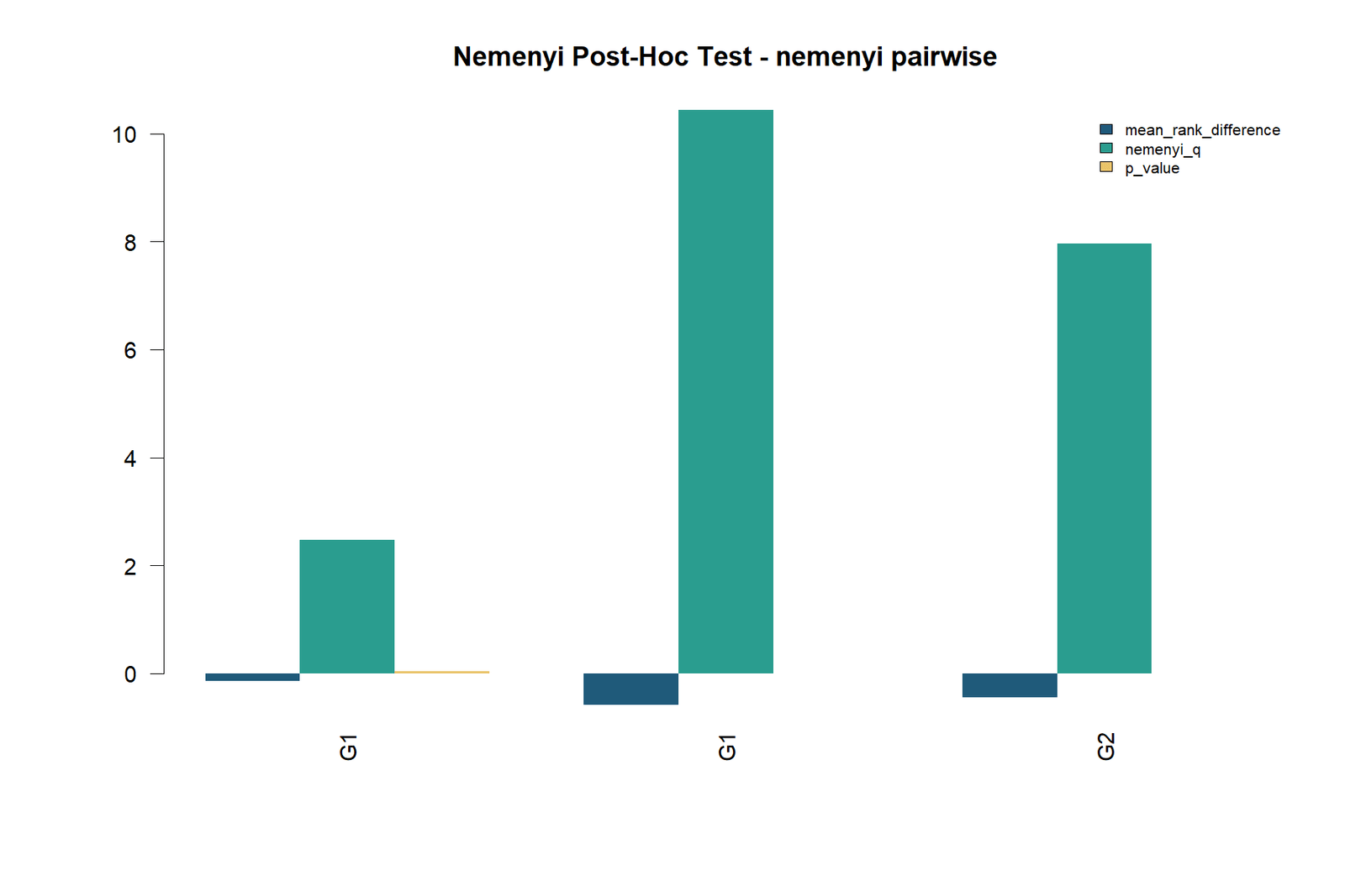
R chart 3: Nemenyi pairwise comparisons
The chart emphasizes the same contrast hierarchy: G1-G3 is largest, G2-G3 is second, and G1-G2 is smallest. The familywise threshold still declares the smallest contrast significant.
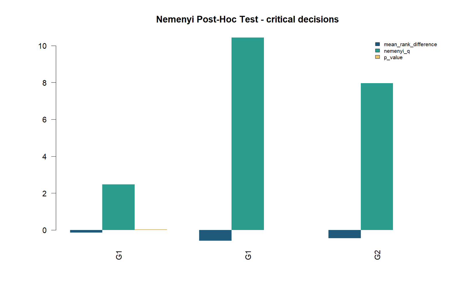
R chart 4: critical decisions
All pairwise absolute mean-rank differences exceed the α = .05 critical difference. The decision pattern is identical across R, Python and the formula-driven workbook.
R chart 5: verified summary
The R summary provides an independent implementation check. Minor last-decimal and extreme-tail p-value differences are expected; the inferential quantities and conclusions agree.
Additional software context is available in statistical analysis in R, ANOVA in R and regression in R.
Nemenyi test in SPSS
SPSS verifies the Friedman structure, but its native pairwise output should not be mislabeled as Nemenyi.
A careful Nemenyi test SPSS workflow distinguishes three layers: the native Friedman omnibus test, optional native pairwise sensitivity tests, and the studentized-range Nemenyi calculation reproduced through verified constants or R/Python integration.
What the supplied SPSS output verifies
The SPSS PDF confirms 649 complete rows, raw descriptive statistics, mean ranks of 1.76, 1.90 and 2.34, and a Friedman statistic of 167.328 with two degrees of freedom and p < .001. It also reports paired Wilcoxon tests for G1-G2, G2-G3 and G1-G3. Those Wilcoxon results are useful sensitivity checks but are not the Nemenyi post hoc test.
The final SPSS page records the independently verified Nemenyi constants: standard error 0.055512738, critical q 2.343700586 and critical difference 0.130105237. This separation prevents a common reporting error in which any SPSS pairwise table following Friedman is automatically called “Nemenyi.”
Recommended SPSS workflow
- Use Analyze → Nonparametric Tests → Related Samples to run Friedman and inspect the rank table.
- Confirm all selected variables represent the same repeated construct and the same 649 cases.
- Save or export the mean ranks.
- Calculate the verified Nemenyi q and critical difference through Python/R integration or the supplied workbook.
- Report the exact method used, rather than relying only on a generic “pairwise comparisons” label.
* Confirm the repeated-measures omnibus result and descriptive statistics.
NPAR TESTS
/FRIEDMAN = G1 G2 G3
/STATISTICS DESCRIPTIVES QUARTILES
/MISSING ANALYSIS.* Optional paired Wilcoxon sensitivity checks; these are not the Nemenyi test.
NPAR TESTS
/WILCOXON = G1 WITH G2 (PAIRED)
G1 WITH G3 (PAIRED)
G2 WITH G3 (PAIRED)
/MISSING ANALYSIS.
* Nemenyi constants used for this verified 649-block, 3-occasion example.
COMPUTE n_blocks = 649.
COMPUTE k_occasions = 3.
COMPUTE q_critical_alpha_05 = 2.3437005863784077.
COMPUTE standard_error = SQRT(k_occasions*(k_occasions+1)/(6*n_blocks)).
COMPUTE critical_difference = q_critical_alpha_05*standard_error.
FORMATS standard_error critical_difference (F12.9).
EXECUTE.
* Native SPSS Friedman pairwise output should not automatically be relabeled
* as Nemenyi. Obtain studentized-range p-values through R/Python integration
* or report the verified q and critical-difference decisions shown here.
For readers who work mainly in SPSS, review categorical data analysis in SPSS, ANOVA in SPSS, t tests in SPSS and regression in SPSS. The menu paths differ, but careful labeling of omnibus and post hoc procedures is equally important.
Nemenyi test in Excel
The supplied Nemenyi test workbook separates raw values, row-level ranks, calculations, diagnostics and reporting.
The Nemenyi test Excel workbook functions as an auditable calculator. It contains Guide, Data_Input, Working, Calculations, Diagnostics and Reporting sheets, so every reported constant can be traced back to the 649 raw rows.
Example layout (raw grades in A5:C653):D5: =RANK.AVG(A5,$A5:$C5,1)
E5: =RANK.AVG(B5,$A5:$C5,1)
F5: =RANK.AVG(C5,$A5:$C5,1)
Copy D5:F5 through row 653.
Mean rank G1: =AVERAGE(D5:D653)
Mean rank G2: =AVERAGE(E5:E653)
Mean rank G3: =AVERAGE(F5:F653)
n: =COUNT(A5:A653)
k: =3
Standard error: =SQRT(k*(k+1)/(6*n))
Critical q: =2.3437005863784077
Critical difference: =Critical_q*Standard_error
Pair q: =ABS(MeanRank_1-MeanRank_2)/Standard_error
Decision: =IF(ABS(MeanRank_1-MeanRank_2)>Critical_difference,"Significant","Not significant")
Data_Input
Store only the unchanged G1, G2 and G3 values. Do not mix manually calculated ranks into the source area. The raw-data boundary makes later corrections and verification safer.
Working
Use RANK.AVG across each row so ties receive average positions. Check that each row’s three ranks total 6 and that the full rank sums total 3,894.
Calculations
Calculate rank sums, mean ranks, the standard error, critical q, critical difference, pairwise q values and Boolean reject decisions. Formula cells should remain linked to the working ranks.
Diagnostics
Document the block structure, tie rule and method identity. A workbook is more trustworthy when assumptions and data lineage are visible rather than implied.
Reporting
Compare calculated constants against independent reference values and display absolute differences. In the supplied workbook, all three audited differences are zero.
P-value limitation
Standard Excel does not provide a direct inverse or survival function for the studentized range. Use the verified critical q for the defined k and α, or calculate p-values in R/Python while retaining Excel for the critical-difference audit.
Nemenyi test compared with Dunn, Conover, Wilcoxon and Tukey
Nemenyi test comparisons and similar post hoc labels can hide different designs and null hypotheses.
Choosing between the Nemenyi test and another post hoc procedure requires matching the dependence structure, omnibus test and scientific estimand.
| Procedure | Typical design | What is compared | Multiplicity approach | Key distinction |
|---|---|---|---|---|
| Friedman-Nemenyi | Repeated / blocked | All condition mean-rank pairs | Studentized range | Procedure used in this article |
| Dunn’s test | Usually independent groups after Kruskal-Wallis; Dunn-style variants also appear in software | Rank-sum contrasts | Bonferroni, Holm or other p adjustment | Do not assume every SPSS Friedman pairwise table is Nemenyi |
| Conover post hoc | Independent or blocked version depending on function | Rank contrasts with a different standardization | Adjusted pairwise p-values | Often more powerful, but not numerically interchangeable |
| Pairwise Wilcoxon | Two related conditions per comparison | Distribution of paired differences | Holm/Bonferroni applied across pairs | Uses original pairwise differences rather than all-condition mean ranks |
| Tukey HSD | Parametric independent-group ANOVA | Arithmetic means | Studentized range | Parametric mean-comparison analogue, not a rank test |
| Nemenyi-Damico-Wolfe-Dunn | Independent samples | Stochastic ordering across groups | Test-specific joint ranking | A separate method despite the shared surname |
Nemenyi vs Dunn test
The phrase “Nemenyi vs Dunn test” cannot be answered without design context. After a Kruskal-Wallis test, Dunn’s method is widely used for independent groups, while an independent-samples Nemenyi procedure is another option. After Friedman, the blocked Nemenyi method compares all repeated-condition mean ranks. Software may implement Dunn-style Friedman comparisons with multiplicity adjustment; those results should be named accurately.
Nemenyi vs pairwise Wilcoxon
Pairwise Wilcoxon signed-rank tests use only the two conditions in each contrast and assess paired differences. The Nemenyi result depends on the common rank system across all k conditions. This distinction can matter because adding or removing a condition changes the mean-rank framework and critical range. Report which procedure answers the scientific question more directly.
Related guides include Mann-Whitney U, median test, Mood’s median test, Jonckheere-Terpstra trend test and the two-sample Kolmogorov-Smirnov test. These are not replacements for the blocked Nemenyi procedure, but the comparisons clarify how design and hypothesis determine the correct rank method.
Nemenyi test diagnostics, sensitivity checks and limitations
Verify the rank construction and interpret small margins cautiously.
A defensible Nemenyi test report does more than repeat adjusted p-values. It checks complete blocks, ties, rank totals, critical-value scaling, original distributions and the stability of conclusions.
Essential computational checks
Substantive sensitivity checks
Borderline pair
G1-G2 exceeded the critical difference by only 0.007029. This does not invalidate the result, but it makes the conclusion more sensitive to data exclusions, changed tie handling or a different family definition than the two G3 comparisons.
Large-sample significance
With 649 blocks, small rank separations can be significant. Statistical detection should not be confused with educational importance. The original mean difference between G1 and G2 was about 0.17 grade points.
Pool dependence
Mean-rank post hoc comparisons are defined relative to the full condition set. A comparison between G1 and G2 can change if the pool of included conditions changes, which is one reason to prespecify the analysis family.
Incomplete blocks
Listwise deletion may discard participants with partial data. When missingness is substantial or informative, a mixed model or another incomplete-block method may better use the available observations.
Shape interpretation
A higher mean rank indicates more frequent relative ordering, not necessarily a constant location shift. Different spreads or crossing distributions can produce rank differences that require cautious wording.
No pairwise effect size
The q statistic is a standardized decision statistic, not a generally interpretable effect size. Report original summaries, mean-rank differences and, where appropriate, separate paired effect-size estimates.
General statistical safeguards are reviewed in p-value interpretation, effect size, Type I and Type II errors, statistical power and parametric versus nonparametric tests.
How to report the Nemenyi test in APA style
Name the omnibus test, pairwise method, mean ranks and multiplicity-aware decisions.
An APA-style Nemenyi test interpretation should not present isolated pairwise p-values without the preceding Friedman result and the direction shown by condition mean ranks.
Recommended APA-style paragraph
A Friedman test indicated that grades differed across G1, G2 and G3, χ²(2, N = 649) = 167.33, p < .001, Kendall’s W = .129. Nemenyi all-pairs comparisons were conducted using a studentized-range critical difference of 0.130. Mean ranks were 1.761 for G1, 1.898 for G2 and 2.341 for G3. G2 ranked higher than G1, mean-rank difference = 0.137, q = 2.470, p = .036; G3 ranked higher than G1, difference = 0.579, q = 10.436, p < .001; and G3 ranked higher than G2, difference = 0.442, q = 7.966, p < .001.
Compact technical report
The Friedman-Nemenyi analysis used 649 complete blocks and three conditions. The common standard error was 0.055513, qcritical was 2.343701, and CD was 0.130105 at α = .05. All absolute mean-rank differences exceeded CD. The pairwise ordering was G3 > G2 > G1.
Reporting checklist
Nemenyi test PDF, Excel and software downloads
Use the reports to reproduce calculations and the workbook to audit every formula.
These Nemenyi test downloads contain the verified Python report, R report, SPSS output and formula-driven Excel workbook used throughout the worked example.
R PDF reportIndependent studentized-range implementation and charts.Open R PDF →
SPSS output PDFFriedman ranks, descriptives, sensitivity tests and verified constants.Open SPSS PDF →
Worked Excel analysisRaw data, ranks, formulas, diagnostics and reporting checks.Download Excel →
Nemenyi test FAQs
Answers to common search and interpretation questions.
What is the Nemenyi test?
The Nemenyi test is a nonparametric all-pairs multiple-comparison procedure. In a Friedman design, it compares the mean ranks of repeated conditions after the omnibus Friedman test rejects equality across all conditions.
Is the Nemenyi test a post hoc test?
Yes. The Friedman-Nemenyi test is usually interpreted after a significant Friedman result. The omnibus test establishes that at least one condition differs; Nemenyi identifies which mean-rank pairs cross the familywise threshold.
What is the Nemenyi test formula?
The workbook-scale statistic is qij = |R̄i − R̄j| / √[k(k + 1)/(6n)]. It is compared with a critical q obtained from the studentized-range distribution, or the mean-rank difference is compared with CD = qcritical × SE.
Does the Nemenyi test assume equal variance?
No classical equal-variance assumption is imposed on the raw conditions. Nevertheless, strong distribution-shape differences can complicate a simple location interpretation, so original distributions and descriptive summaries should be reported.
Does the Nemenyi test require normality?
No. It is rank based. Its important conditions are a valid repeated or blocked design, independent blocks, ordered outcomes, consistent measurement and appropriate treatment of ties and missing values.
How do I perform a Nemenyi test in R?
For complete blocked data after Friedman, install PMCMRplus and use frdAllPairsNemenyiTest(as.matrix(wide_data)). Use kwAllPairsNemenyiTest() only for the independent-group Kruskal-Wallis setting.
Why does R say it could not find posthoc.friedman.nemenyi.test?
The function name may come from older code or an unloaded package. In current PMCMRplus workflows, use PMCMRplus::frdAllPairsNemenyiTest(). Loading the package or using the explicit namespace resolves the usual function-not-found problem.
How do I run the Nemenyi test in Python?
Rank every row with average ties, calculate condition mean ranks, compute SE = √[k(k + 1)/(6n)], and use SciPy’s studentized-range distribution for the critical value and adjusted p-values. The code in this guide includes the required √2 scaling.
Can SPSS run a native Nemenyi post hoc test?
SPSS can run Friedman and produce native pairwise comparisons, but those outputs should not automatically be labeled Nemenyi. A verified Nemenyi analysis can be completed through R/Python integration or a formula-driven workbook using the SPSS mean ranks.
Can Excel calculate the Nemenyi test?
Yes for ranks, mean-rank differences, q statistics and critical-difference decisions. Standard Excel lacks a native studentized-range p-value function, so the critical q must come from a verified source or exact p-values can be calculated in R or Python.
What is the difference between the Nemenyi test and Dunn’s test?
They use different standardizations and are commonly tied to different designs. Dunn’s test is widely used after Kruskal-Wallis for independent groups, while the analysis here is the blocked Nemenyi test after Friedman. Always match the procedure to the omnibus design.
What is the difference between Friedman-Nemenyi and Kruskal-Nemenyi?
Friedman-Nemenyi analyzes related conditions or complete blocks. Kruskal-Nemenyi analyzes independent groups after Kruskal-Wallis. Their R functions and standard errors are not interchangeable.
What does the critical difference mean?
The critical difference is the smallest absolute separation between two condition mean ranks required for significance at the chosen familywise alpha. In this example CD = 0.130105.
Why do Python and R show different extremely small p-values?
Numerical algorithms and floating-point tail precision differ. Python underflowed the smallest p-value to zero, while R retained a very small positive value. Because both q statistics are far beyond the critical threshold, the scientific decisions are identical.
Is the Nemenyi test significant for G1 versus G2?
Yes in this worked dataset. The absolute mean-rank difference was 0.137134, slightly larger than CD = 0.130105; q = 2.470317 and adjusted p = .035991. It is the narrowest of the three significant comparisons.
How should I interpret all three significant pairs?
Report the ordering and relative magnitudes: G3 had the highest mean rank, G2 was intermediate and G1 was lowest. The G1-G3 and G2-G3 separations were much larger than G1-G2, so “all significant” does not mean “equally different.”