
.cix-article{–ink:#102238;–muted:#52657a;–line:#dce5ed;–paper:#fff;–soft:#f4f8fb;–navy:#092a45;–teal:#0d7774;–cyan:#dff7f6;–amber:#f4a340;–amber-soft:#fff4df;–red:#a83232;–red-soft:#fff0f0;–green:#176b47;–green-soft:#e9f8f0;–violet:#6654b8;–violet-soft:#f0edff;–shadow:0 16px 45px rgba(18,44,67,.10);font-family:Inter,ui-sans-serif,system-ui,-apple-system,BlinkMacSystemFont,”Segoe UI”,Arial,sans-serif;color:var(–ink);line-height:1.72;width:auto;max-width:none!important;margin-left:calc(50% – 50vw + 12px)!important;margin-right:calc(50% – 50vw + 12px)!important;margin-top:0!important;margin-bottom:0!important;background:var(–paper);font-size:17px;overflow-x:clip}
.cix-article *{box-sizing:border-box}.cix-article a{color:#075f72;text-decoration-thickness:1px;text-underline-offset:3px}.cix-article a:hover{color:#043f4c}.cix-shell{width:100%;max-width:1480px;margin:0 auto;padding:clamp(18px,2.8vw,42px)}.cix-hero{position:relative;overflow:hidden;border-radius:28px;background:linear-gradient(132deg,#07263f 0%,#0b4b61 55%,#0a7770 100%);color:#fff;padding:clamp(28px,6vw,68px);box-shadow:var(–shadow)}.cix-hero:before{content:””;position:absolute;right:-90px;top:-120px;width:360px;height:360px;border-radius:50%;background:rgba(255,255,255,.07)}.cix-hero:after{content:””;position:absolute;left:-110px;bottom:-180px;width:390px;height:390px;border-radius:50%;background:rgba(244,163,64,.10)}.cix-hero>*{position:relative;z-index:1}.cix-kicker{display:inline-flex;align-items:center;gap:9px;padding:7px 12px;border:1px solid rgba(255,255,255,.25);border-radius:999px;background:rgba(255,255,255,.09);font-size:.78rem;font-weight:800;letter-spacing:.08em;text-transform:uppercase}.cix-kicker i{width:9px;height:9px;border-radius:50%;background:#ffbd62;box-shadow:0 0 0 5px rgba(255,189,98,.16)}.cix-hero h1{font-size:clamp(2.15rem,5.2vw,4.65rem);line-height:1.04;letter-spacing:-.045em;margin:22px 0 18px;max-width:1000px;color:#fff}.cix-hero .cix-lead{font-size:clamp(1.05rem,2vw,1.34rem);max-width:900px;color:#e9f7fb;margin:0}.cix-badges{display:flex;flex-wrap:wrap;gap:10px;margin-top:25px}.cix-badge{padding:8px 12px;border-radius:999px;background:rgba(255,255,255,.11);border:1px solid rgba(255,255,255,.19);font-size:.84rem;font-weight:750}.cix-hero-result{margin-top:28px;display:grid;grid-template-columns:repeat(4,minmax(0,1fr));gap:12px}.cix-hero-metric{background:rgba(255,255,255,.10);border:1px solid rgba(255,255,255,.16);border-radius:16px;padding:14px}.cix-hero-metric span{display:block;color:#cdeaf0;font-size:.78rem;text-transform:uppercase;letter-spacing:.05em;font-weight:800}.cix-hero-metric strong{display:block;margin-top:4px;font-size:1.28rem;color:#fff}.cix-ad{display:flex;align-items:center;justify-content:center;min-height:96px;margin:26px 0;border:1px dashed #b8c6d1;border-radius:18px;background:#f8fafc;color:#718096;font-size:.78rem;letter-spacing:.14em;text-transform:uppercase}.cix-quick{display:grid;grid-template-columns:1.35fr .65fr;gap:20px;margin:28px 0}.cix-card{min-width:0;max-width:100%;border:1px solid var(–line);border-radius:22px;background:#fff;box-shadow:0 10px 30px rgba(21,48,70,.06);padding:clamp(19px,3vw,30px)}.cix-card h2,.cix-card h3{margin-top:0}.cix-answer{background:linear-gradient(145deg,#f2fbfa,#fff);border-color:#bfe5e2}.cix-answer .cix-verdict{display:inline-flex;align-items:center;gap:9px;padding:8px 12px;border-radius:999px;background:var(–green-soft);color:var(–green);font-weight:850;font-size:.84rem}.cix-answer .cix-verdict:before{content:”✓”;display:grid;place-items:center;width:22px;height:22px;border-radius:50%;background:var(–green);color:#fff}.cix-answer h2{font-size:clamp(1.55rem,3vw,2.25rem);line-height:1.15;margin:15px 0 10px}.cix-mini-table{display:grid;gap:10px}.cix-mini-row{display:flex;justify-content:space-between;gap:20px;padding:11px 0;border-bottom:1px solid var(–line)}.cix-mini-row:last-child{border-bottom:0}.cix-mini-row span{color:var(–muted)}.cix-mini-row strong{text-align:right}.cix-toc{margin:26px 0;border-radius:22px;background:var(–navy);color:#fff;padding:24px}.cix-toc h2{color:#fff;margin:0 0 14px;font-size:1.2rem}.cix-toc-grid{display:grid;grid-template-columns:repeat(3,minmax(0,1fr));gap:8px 20px}.cix-toc a{color:#d9f6f5;text-decoration:none;padding:7px 0;display:block;border-bottom:1px solid rgba(255,255,255,.12)}.cix-toc a:hover{color:#fff}.cix-section{scroll-margin-top:24px;margin:54px 0}.cix-section-head{display:grid;grid-template-columns:auto 1fr;align-items:start;gap:14px;margin-bottom:20px}.cix-num{width:42px;height:42px;border-radius:13px;background:var(–navy);color:#fff;display:grid;place-items:center;font-weight:900}.cix-section-head h2{margin:0;font-size:clamp(1.65rem,3.4vw,2.65rem);line-height:1.15;letter-spacing:-.025em}.cix-section-head p{grid-column:2;margin:5px 0 0;color:var(–muted);max-width:920px}.cix-grid-2{display:grid;grid-template-columns:repeat(2,minmax(0,1fr));gap:20px}.cix-grid-2>*,.cix-grid-3>*,.cix-grid-4>*,.cix-chart-grid>*,.cix-downloads>*,.cix-related>*,.cix-quick>*{min-width:0}.cix-grid-3{display:grid;grid-template-columns:repeat(3,minmax(0,1fr));gap:18px}.cix-grid-4{display:grid;grid-template-columns:repeat(4,minmax(0,1fr));gap:14px}.cix-callout{border-radius:18px;padding:18px 20px;border-left:5px solid var(–teal);background:var(–cyan);margin:20px 0}.cix-callout strong{color:#084f4c}.cix-note{border-left-color:var(–amber);background:var(–amber-soft)}.cix-note strong{color:#875311}.cix-formula{border:1px solid #cbd8e3;background:linear-gradient(180deg,#fff,#f7fafc);border-radius:20px;padding:22px;margin:18px 0;text-align:center;overflow:visible}.cix-formula .eq{font-family:”Cambria Math”,”Times New Roman”,serif;font-size:clamp(1.08rem,2.2vw,1.5rem);white-space:normal;overflow-wrap:anywhere;word-break:normal;line-height:1.55}.cix-formula p{margin:8px auto 0;color:var(–muted);max-width:850px;text-align:left;font-size:.94rem}.cix-pill-list{display:flex;flex-wrap:wrap;gap:10px;margin:15px 0}.cix-pill{background:var(–soft);border:1px solid var(–line);border-radius:999px;padding:8px 12px;font-weight:750;font-size:.88rem}.cix-flow{display:grid;grid-template-columns:repeat(5,minmax(0,1fr));gap:10px;counter-reset:flow}.cix-step{position:relative;padding:18px 14px 16px;border:1px solid var(–line);border-radius:18px;background:#fff;min-height:148px}.cix-step:before{counter-increment:flow;content:counter(flow);display:grid;place-items:center;width:30px;height:30px;border-radius:10px;background:var(–teal);color:#fff;font-weight:900;margin-bottom:10px}.cix-step h3{font-size:1rem;margin:0 0 6px}.cix-step p{font-size:.9rem;color:var(–muted);margin:0}.cix-table-wrap{min-width:0;max-width:100%;overflow-x:auto;border:1px solid var(–line);border-radius:18px;background:#fff}.cix-table{width:100%;border-collapse:collapse;min-width:720px}.cix-table.cix-compact{min-width:0}.cix-table th{background:var(–navy);color:#fff;text-align:left;padding:13px 14px;font-size:.85rem;letter-spacing:.02em}.cix-table td{padding:13px 14px;border-bottom:1px solid var(–line);vertical-align:top}.cix-table tbody tr:nth-child(even){background:#f8fafc}.cix-table tbody tr:last-child td{border-bottom:0}.cix-stat-grid{display:grid;grid-template-columns:repeat(4,minmax(0,1fr));gap:12px;margin:16px 0}.cix-stat{border:1px solid var(–line);border-radius:16px;padding:16px;background:#fff}.cix-stat span{display:block;color:var(–muted);font-size:.78rem;font-weight:800;text-transform:uppercase;letter-spacing:.05em}.cix-stat strong{display:block;font-size:1.34rem;margin-top:4px}.cix-stat small{display:block;color:var(–muted);margin-top:4px}.cix-result-panel{border-radius:22px;background:linear-gradient(145deg,#082c47,#0b5966);color:#fff;padding:26px}.cix-result-panel h3{color:#fff;margin-top:0;font-size:1.45rem}.cix-result-panel p{color:#e5f6f7}.cix-result-panel .cix-result-big{font-size:clamp(2rem,5vw,3.7rem);line-height:1;font-weight:950;color:#fff;margin:10px 0}.cix-result-panel .cix-result-tag{display:inline-block;padding:8px 12px;border-radius:999px;background:rgba(255,255,255,.12);border:1px solid rgba(255,255,255,.18);font-weight:800}.cix-figure{min-width:0;max-width:100%;margin:0;border:1px solid var(–line);border-radius:22px;overflow:hidden;background:#fff;box-shadow:0 10px 30px rgba(21,48,70,.06)}.cix-figure img{display:block;width:100%;height:auto;background:#f3f6f8}.cix-figure figcaption{padding:18px 20px}.cix-figure h3{font-size:1.08rem;margin:0 0 6px}.cix-figure p{margin:0;color:var(–muted);font-size:.94rem}.cix-chart-grid{display:grid;grid-template-columns:repeat(2,minmax(0,1fr));gap:20px}.cix-chart-grid .cix-wide{grid-column:1/-1}.cix-code{min-width:0;max-width:100%;position:relative;background:#071d2d;color:#e6f2f7;border-radius:18px;overflow:auto;padding:20px;margin:16px 0;box-shadow:inset 0 0 0 1px rgba(255,255,255,.07)}.cix-code code{display:block;white-space:pre;min-width:max-content;font-family:”SFMono-Regular”,Consolas,”Liberation Mono”,monospace;font-size:.88rem;line-height:1.65}.cix-code-label{display:inline-block;margin-bottom:8px;color:#7ee7db;font-size:.76rem;font-weight:900;letter-spacing:.08em;text-transform:uppercase}.cix-downloads{display:grid;grid-template-columns:repeat(4,minmax(0,1fr));gap:14px}.cix-download{display:flex;flex-direction:column;min-height:190px;padding:20px;border-radius:20px;border:1px solid var(–line);background:#fff;text-decoration:none!important;color:var(–ink)!important;box-shadow:0 10px 30px rgba(21,48,70,.06);transition:.2s transform,.2s box-shadow}.cix-download:hover{transform:translateY(-3px);box-shadow:0 16px 38px rgba(21,48,70,.12)}.cix-file-icon{width:46px;height:46px;border-radius:14px;display:grid;place-items:center;background:var(–violet-soft);color:var(–violet);font-weight:950;margin-bottom:16px}.cix-download strong{font-size:1.05rem}.cix-download span{color:var(–muted);font-size:.88rem;margin-top:6px}.cix-download em{margin-top:auto;padding-top:16px;color:#075f72;font-style:normal;font-weight:850}.cix-checks{display:grid;gap:10px}.cix-check{position:relative;padding:13px 14px 13px 44px;border:1px solid var(–line);border-radius:15px;background:#fff}.cix-check:before{content:”✓”;position:absolute;left:14px;top:13px;width:22px;height:22px;border-radius:50%;display:grid;place-items:center;background:var(–green-soft);color:var(–green);font-weight:950}.cix-faq details{border:1px solid var(–line);border-radius:17px;background:#fff;margin:11px 0;overflow:hidden}.cix-faq summary{cursor:pointer;font-weight:850;padding:17px 20px;list-style:none}.cix-faq summary::-webkit-details-marker{display:none}.cix-faq summary:after{content:”+”;float:right;color:var(–teal);font-size:1.4rem;line-height:1}.cix-faq details[open] summary:after{content:”−”}.cix-faq .cix-faq-answer{padding:0 20px 18px;color:var(–muted)}.cix-related{display:grid;grid-template-columns:repeat(3,minmax(0,1fr));gap:12px}.cix-related a{display:block;border:1px solid var(–line);border-radius:15px;padding:14px 16px;background:#fff;text-decoration:none;font-weight:800}.cix-footer-note{border-radius:22px;background:var(–soft);border:1px solid var(–line);padding:22px;color:var(–muted)}.cix-back{display:inline-flex;align-items:center;gap:8px;border-radius:999px;background:var(–navy);color:#fff!important;text-decoration:none!important;padding:11px 16px;font-weight:850;margin-top:18px}.cix-sr{position:absolute!important;width:1px!important;height:1px!important;padding:0!important;margin:-1px!important;overflow:hidden!important;clip:rect(0,0,0,0)!important;white-space:nowrap!important;border:0!important}
@media(max-width:960px){.cix-hero-result,.cix-grid-4,.cix-stat-grid,.cix-downloads{grid-template-columns:repeat(2,minmax(0,1fr))}.cix-toc-grid,.cix-grid-3,.cix-related{grid-template-columns:repeat(2,minmax(0,1fr))}.cix-flow{grid-template-columns:repeat(2,minmax(0,1fr))}.cix-flow .cix-step:last-child{grid-column:1/-1}.cix-quick{grid-template-columns:1fr}}
@media(max-width:680px){.cix-article{font-size:16px;margin-left:calc(50% – 50vw + 6px)!important;margin-right:calc(50% – 50vw + 6px)!important}.cix-shell{padding:12px}.cix-hero{border-radius:20px;padding:26px 20px}.cix-hero h1{font-size:2.2rem}.cix-hero-result,.cix-grid-2,.cix-grid-3,.cix-grid-4,.cix-stat-grid,.cix-downloads,.cix-chart-grid,.cix-toc-grid,.cix-related,.cix-flow{grid-template-columns:1fr}.cix-chart-grid .cix-wide,.cix-flow .cix-step:last-child{grid-column:auto}.cix-card{border-radius:18px;padding:18px}.cix-section{margin:42px 0}.cix-section-head{grid-template-columns:36px 1fr;gap:11px}.cix-num{width:36px;height:36px}.cix-section-head p{grid-column:1/-1}.cix-table{min-width:650px}.cix-formula{padding:18px 12px;text-align:left}.cix-formula .eq{font-size:1.05rem}.cix-mini-row{align-items:flex-start;flex-direction:column;gap:2px}.cix-mini-row strong{text-align:left}}
.cix-seo-context{font-size:1.02rem;color:#31475d;margin:-5px 0 20px;max-width:1180px}
.cix-model{display:grid;grid-template-columns:1.05fr .95fr;gap:20px;align-items:stretch}
.cix-model .cix-card{height:100%}
.cix-hypothesis{border:1px solid var(–line);border-radius:18px;padding:20px;background:#fff}
.cix-hypothesis h3{margin:0 0 10px}
.cix-direction{display:grid;grid-template-columns:repeat(3,minmax(0,1fr));gap:12px;margin:16px 0}
.cix-direction>div{border:1px solid var(–line);border-radius:16px;padding:16px;background:var(–soft)}
.cix-keyword-box{border:1px solid #b9d8e2;border-radius:20px;background:linear-gradient(145deg,#eff9fc,#fff);padding:22px;margin:22px 0}
.cix-keyword-box h3{margin-top:0}
.cix-equation-lines{display:grid;gap:10px;text-align:left}
.cix-equation-line{display:grid;grid-template-columns:minmax(140px,.38fr) 1fr;gap:16px;align-items:start;padding:10px 0;border-bottom:1px solid var(–line)}
.cix-equation-line:last-child{border-bottom:0}
.cix-equation-line strong{color:var(–navy)}
@media(max-width:900px){.cix-model,.cix-direction{grid-template-columns:1fr}.cix-equation-line{grid-template-columns:1fr;gap:4px}}
.cix-pair-significant{background:#eefaf3!important}.cix-pair-nonsig{background:#fff9ed!important}.cix-rankbar{height:10px;border-radius:999px;background:linear-gradient(90deg,#0d7774,#4ca9a4);margin-top:8px}.cix-holm-step{display:grid;grid-template-columns:60px 1.2fr 1fr 1fr 1fr;gap:10px;align-items:center;padding:12px 0;border-bottom:1px solid var(–line)}.cix-holm-step:last-child{border-bottom:0}.cix-holm-step strong{color:var(–navy)}.cix-inline-code{font-family:”SFMono-Regular”,Consolas,monospace;background:#eef4f8;border:1px solid var(–line);padding:2px 6px;border-radius:7px;font-size:.9em}.cix-definition{display:grid;grid-template-columns:minmax(170px,.35fr) 1fr;gap:16px;padding:12px 0;border-bottom:1px solid var(–line)}.cix-definition:last-child{border-bottom:0}.cix-definition strong{color:var(–navy)}@media(max-width:720px){.cix-holm-step{grid-template-columns:1fr;gap:2px}.cix-definition{grid-template-columns:1fr;gap:4px}}
Conover Test: 7 Essential Steps, Formula and Worked Example
The Conover test, also called the Conover-Iman test, is a rank-based post hoc procedure for finding which independent groups differ after a significant Kruskal-Wallis test. This complete guide explains the Conover test formula, assumptions, pooled-rank calculations, Holm adjustment, exact pairwise interpretation, and reproducible workflows in Python, R, SPSS and Excel.
Four independent groups
Tie-corrected ranks
Holm adjustment
Python + R + SPSS + Excel
The Conover test identified four significant study-time group differences.
In this worked Conover test example, final grade (G3) was compared across four independent studytime groups. The tie-corrected Kruskal-Wallis test was significant, H(3) = 50.3162, p = 6.84 × 10⁻¹¹, so pairwise Conover-Iman comparisons were justified. After Holm correction, groups 1 vs 2, 1 vs 3, 1 vs 4, and 2 vs 3 differed significantly. Groups 2 vs 4 and 3 vs 4 did not.
What does the Conover test measure?
A post hoc comparison of pooled mean ranks after a significant independent-samples omnibus test.
The Conover test answers the question left unresolved by Kruskal-Wallis: once the global null hypothesis has been rejected, exactly which pairs of independent groups differ? It compares pooled rank sums or mean ranks, uses the variability of the complete rank set, and evaluates every pair with a t reference distribution.
The Conover test is therefore a focused answer to a multiple-comparison problem: it converts one significant omnibus result into a controlled set of interpretable pairwise conclusions.
The statistical question
Suppose a researcher has three or more independent groups and an ordinal or continuous outcome. The Kruskal-Wallis test can indicate that the groups are not all drawn from the same distributional location, but it does not identify the responsible pairs. The Conover test performs those pairwise follow-ups.
For group i and group j, the method compares their average pooled ranks. A large absolute mean-rank difference produces a large absolute Conover t statistic. The raw pairwise p-values are then adjusted to control the multiplicity created by testing several pairs.
What the Conover test does not automatically prove
A significant result is not automatically a difference in arithmetic means or medians. Rank tests respond to distributional ordering. If group distributions have similar shapes and differ mainly in location, a location interpretation is reasonable. When shapes cross or spreads differ strongly, the result is better described as a difference in rank distribution or stochastic ordering.
The Conover post hoc test also does not replace the omnibus stage. The intended workflow is Kruskal-Wallis first, Conover-Iman second, and multiplicity adjustment third.
Readers new to ranks may first review percentiles and quartiles, descriptive statistics, and parametric vs nonparametric tests.
When should you use the Conover-Iman test?
All-pairs follow-up comparisons after a rejected Kruskal-Wallis null hypothesis.
The search question when to use the Conover Iman test has a precise answer. Use the procedure when the design contains at least three independent groups, the outcome can be ranked, Kruskal-Wallis is significant, and the research goal is to identify pairwise differences while controlling false positives.
The Conover test should be chosen before examining which pair looks most different, because post hoc method selection based on observed gaps can distort the error rate.
Independent groups?
Each observational unit must belong to one group only.
Three or more?
With only two groups, use a direct two-sample procedure.
Rankable outcome?
The response should be ordinal or continuous.
Omnibus rejected?
The Kruskal-Wallis null should be rejected before pairwise follow-up.
Adjustment selected?
Choose Holm, Bonferroni, BH or another planned correction.
Strong use cases
Situations requiring another method
Conover test assumptions: seven conditions to check
Rank-based methods reduce some distributional requirements but still depend on design and interpretation conditions.
The Conover test assumptions concern independence, measurement scale, group definition, the omnibus result, tie handling, multiplicity and the meaning assigned to rank differences. A defensible post hoc analysis reports these conditions rather than simply listing adjusted p-values.
These Conover test conditions should be checked in the data-management stage and revisited when the final direction of each pair is interpreted.
Independent observations
No student, patient, machine or experimental unit should appear in more than one group. Dependence makes the rank variance and t reference inappropriate.
Independent groups
The categories must be mutually exclusive. In this example, each student has exactly one studytime code from 1 through 4.
Ordinal or continuous outcome
The response must have a meaningful order. G3 is a numeric final grade and therefore can be pooled and ranked.
Meaningful omnibus result
Kruskal-Wallis should reject its global null before the Conover post hoc stage is interpreted.
Ties handled
Tied outcomes receive midranks. The pooled rank variance and omnibus statistic must use the corresponding tie correction.
Multiplicity controlled
Six pairwise tests are produced for four groups. Reporting raw p-values alone would inflate the familywise Type I error rate.
Comparable-shape assumption for a location statement
If the group distributions have similar shapes and spreads, differences in mean rank can be interpreted primarily as differences in location. When empirical cumulative distribution functions cross substantially, a simple “median difference” interpretation is unsafe. The result should instead be described as evidence that one group tends to produce larger or smaller observations over the ranked distribution.
Randomization and generalization
The mathematical test can be calculated on any numbers, but population inference requires an appropriate sampling or assignment process. A convenience sample supports conclusions about the observed dataset more readily than broad claims about all students.
Supporting diagnostics include box plot interpretation, histogram interpretation, frequency distributions, and outlier detection.
Conover test hypotheses: global and pairwise statements
Separate the Kruskal-Wallis omnibus hypotheses from the six Conover-Iman pairwise hypotheses.
The Conover test is a second-stage procedure. First state the global Kruskal-Wallis null; then state the pairwise null for every two studytime groups. This prevents the common mistake of treating one pairwise p-value as though it were the entire analysis.
Omnibus hypotheses
H0,global: G3 has the same distributional location across studytime groups 1, 2, 3 and 4.
H1,global: at least one studytime group differs in distributional location.
The observed tie-corrected statistic was H = 50.3162 with df = 3 and p = 6.84157 × 10⁻¹¹. The global null was therefore rejected at conventional significance levels.
Pairwise hypotheses
For each pair i, j:
H0,ij: groups i and j have equal expected pooled ranks under the Conover-Iman null.
H1,ij: their expected pooled ranks differ.
With four groups there are m = k(k – 1)/2 = 6 pairwise hypotheses. The Holm procedure evaluates all six as one family.
The first listed group has a lower mean rank than the second.
The first listed group has a higher mean rank than the second.
Larger |t| means the mean-rank difference is large relative to its Conover standard error.
Conover test formula, pooled ranks and Holm calculation
The full method combines midranks, a tie-corrected Kruskal-Wallis statistic, pooled rank variance and a t reference with N-k degrees of freedom.
The Conover test formula is often presented without its supporting quantities. The steps below show how the statistic is constructed and why the final p-value differs from a simple pairwise Mann-Whitney calculation.
A transparent Conover test calculation is reproducible from the pooled ranks and does not require a hidden software-only shortcut.
Step 1: pool all observations and assign midranks
Combine all G3 observations, sort them from smallest to largest, and assign ranks 1 through N. Tied final grades receive the average of the ranks they occupy. Let rij be the pooled rank of observation j in group i.
Ri is the rank sum and R̄i is the mean rank for group i.
Step 2: compute the Kruskal-Wallis statistic and tie correction
The shortcut H must be divided by the tie-correction factor C when repeated outcome values are present.
For the G3 data, Σ(t³ – t) = 3,493,782, C = 0.9872191, uncorrected H = 49.6731, and tie-corrected H* = 50.3162.
Step 3: calculate the pooled rank variance
The tie-adjusted pooled rank variance was s² = 34,704.8634. Without ties, the first term alone would equal 35,154.1667.
Step 4: calculate the Conover standard error and t statistic
Here N = 649, k = 4, df = 645, and the omnibus scaling factor (N – 1 – H*)/(N – k) equals 0.9266415.
Step 5: convert t statistics to raw p-values
For a two-sided comparison, each raw p-value is obtained from the Student t distribution with 645 degrees of freedom. The smallest raw p-value belongs to group 1 vs group 3, where t = -6.7256.
Step 6: apply Holm’s step-down correction
Sort the six raw p-values from smallest to largest. Compare the first with α/6, the second with α/5, and so on. Holm-adjusted p-values multiply each ordered p-value by the number of remaining hypotheses while enforcing monotonicity.
Conover test example: final grade across four study-time groups
A complete data dictionary and descriptive profile for the 649-row worked analysis.
This Conover test example compares final grade G3 across four levels of reported weekly study time. The example is large enough to show ties, unequal group sizes, a significant omnibus result and both significant and non-significant post hoc pairs.
The Conover test dataset also demonstrates why descriptive summaries and rank summaries should appear together: readers can see both the original grade scale and the inferential rank scale.
Research scenario
The research question is whether the distributional location of final grades differs across studytime categories. The grouping codes represent increasing study-time bands. Every student contributes one G3 value and one studytime category, so the design is independent rather than repeated.
The analysis includes all 649 complete rows. Because G3 takes integer values from 0 to 19, ties are abundant. The Conover-Iman calculations therefore use pooled midranks and explicit tie correction.
Variables used
| studytime group | n | Mean G3 | SD | Median | Q1 | Q3 | Min-Max | Mean rank |
|---|---|---|---|---|---|---|---|---|
| 1 | 212 | 10.844 | 3.219 | 11 | 10 | 13 | 0-18 | 258.913 |
| 2 | 305 | 12.092 | 3.243 | 12 | 10 | 14 | 0-19 | 338.264 |
| 3 | 97 | 13.227 | 2.502 | 13 | 12 | 15 | 8-18 | 406.758 |
| 4 | 35 | 13.057 | 3.038 | 13 | 11 | 15 | 6-19 | 383.129 |
Conover test statistics, pairwise results and exact interpretation
The complete results table connects every mean-rank contrast to its standard error, t statistic and Holm decision.
The Conover test results below were independently reproduced in the Python report, R report and worked Excel analysis. The strongest result is group 1 vs group 3; the weakest is group 3 vs group 4.
The Conover test table should be read row by row, with the signed mean-rank difference interpreted before the adjusted p-value.
Omnibus result
df = 3, p = 6.84157 × 10⁻¹¹. Reject the global null that all four studytime groups have the same distributional location.
Proceed to Conover-Iman post hoc comparisons
Calculation audit
| Pair | Mean-rank difference | Conover SE | t | Raw p | Holm p | Decision | Direction |
|---|---|---|---|---|---|---|---|
| 1 vs 2 | -79.3512 | 16.0354 | -4.9485 | 9.55463 × 10⁻⁷ | 4.77732 × 10⁻⁶ | Significant | Group 1 lower |
| 1 vs 3 | -147.8450 | 21.9825 | -6.7256 | 3.85878 × 10⁻¹¹ | 2.31527 × 10⁻¹⁰ | Significant | Group 1 lower |
| 1 vs 4 | -124.2158 | 32.7188 | -3.7965 | 0.000160620 | 0.000642478 | Significant | Group 1 lower |
| 2 vs 3 | -68.4938 | 20.9039 | -3.2766 | 0.00110699 | 0.00332098 | Significant | Group 2 lower |
| 2 vs 4 | -44.8646 | 32.0042 | -1.4018 | 0.161445 | 0.322890 | Not significant | No reliable ordering |
| 3 vs 4 | 23.6292 | 35.3605 | 0.6682 | 0.504222 | 0.504222 | Not significant | No reliable ordering |
Why group 1 differs from every other group
Group 1 has the lowest mean rank, 258.91. Its mean-rank gaps from groups 2, 3 and 4 are 79.35, 147.84 and 124.22 rank units. Each gap is large relative to its Conover standard error, so all three adjusted p-values remain below .001.
Why group 4 is uncertain
Group 4 has only 35 observations, so comparisons involving it have larger standard errors. Its mean rank of 383.13 lies between groups 2 and 3. The 2 vs 4 and 3 vs 4 contrasts are therefore not sufficiently precise to reject their pairwise null hypotheses.
Conover test in Python: scikit-posthocs, verification and charts
The Python workflow combines SciPy for Kruskal-Wallis with scikit-posthocs or a transparent manual implementation for Conover-Iman comparisons.
The Conover test in Python can be run with scikit_posthocs.posthoc_conover(). A high-quality workflow first verifies the omnibus result, confirms group order, selects the Holm correction explicitly, and then audits the package output against the formula.
The Python output is most reproducible when the package version and ordered group labels are reported with the results.
import pandas as pd
from scipy import stats
import scikit_posthocs as spdf = pd.read_csv("dataset.csv")
# Omnibus stage
groups = [g["G3"].to_numpy() for _, g in df.groupby("studytime", sort=True)]
kw = stats.kruskal(*groups)
print(kw)
# Conover-Iman pairwise stage with Holm adjustment
p_holm = sp.posthoc_conover(
df,
val_col="G3",
group_col="studytime",
p_adjust="holm",
sort=True
)
print(p_holm)
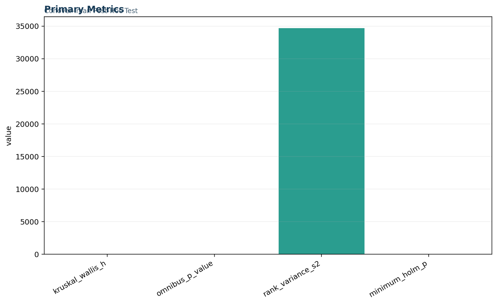
Python primary-metrics summary
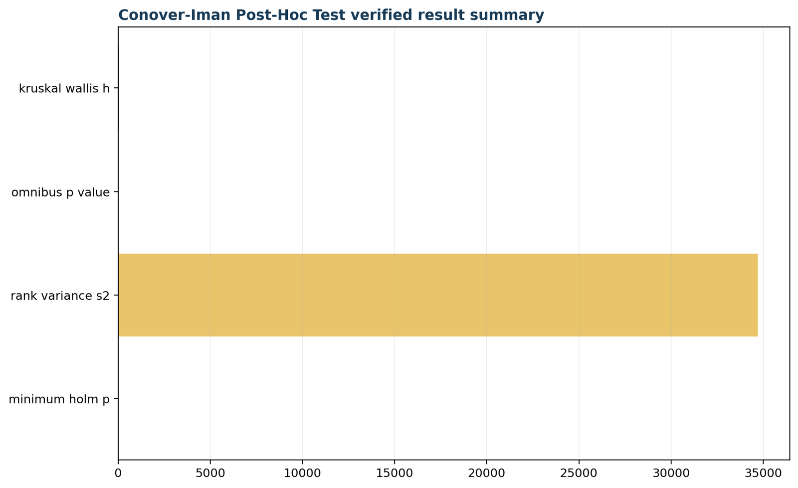
The opening chart consolidates the inferential framework for the Conover test. The omnibus Kruskal–Wallis result was H = 50.316208 with p = 6.84157 × 10⁻¹¹, the pooled rank variance was s² = 34,704.863426, and the smallest Holm-adjusted pairwise p-value was 2.31527 × 10⁻¹⁰. Together, these values show a strong overall group difference and justify examining the six post hoc contrasts.
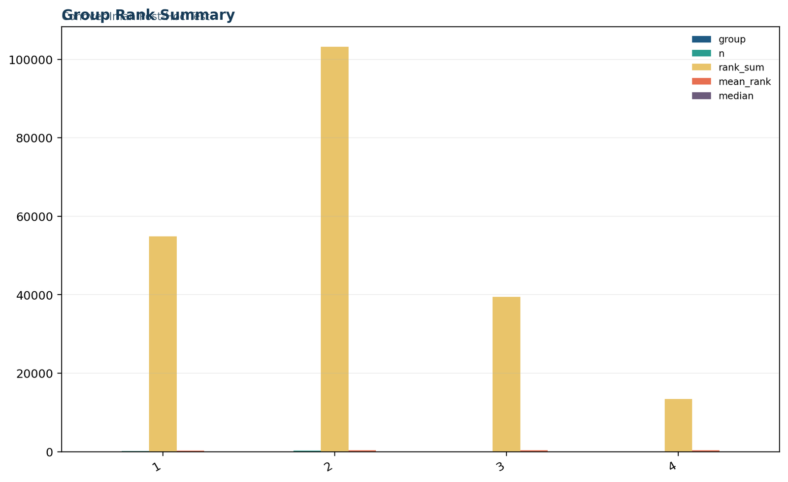
Group rank summary
The mean-rank pattern rises from 258.91 for studytime group 1 to 338.26 for group 2 and 406.76 for group 3, before easing to 383.13 for group 4. Because higher G3 values receive higher pooled ranks, the visual indicates that groups 3 and 4 occupy the upper part of the final-grade distribution more often than group 1.
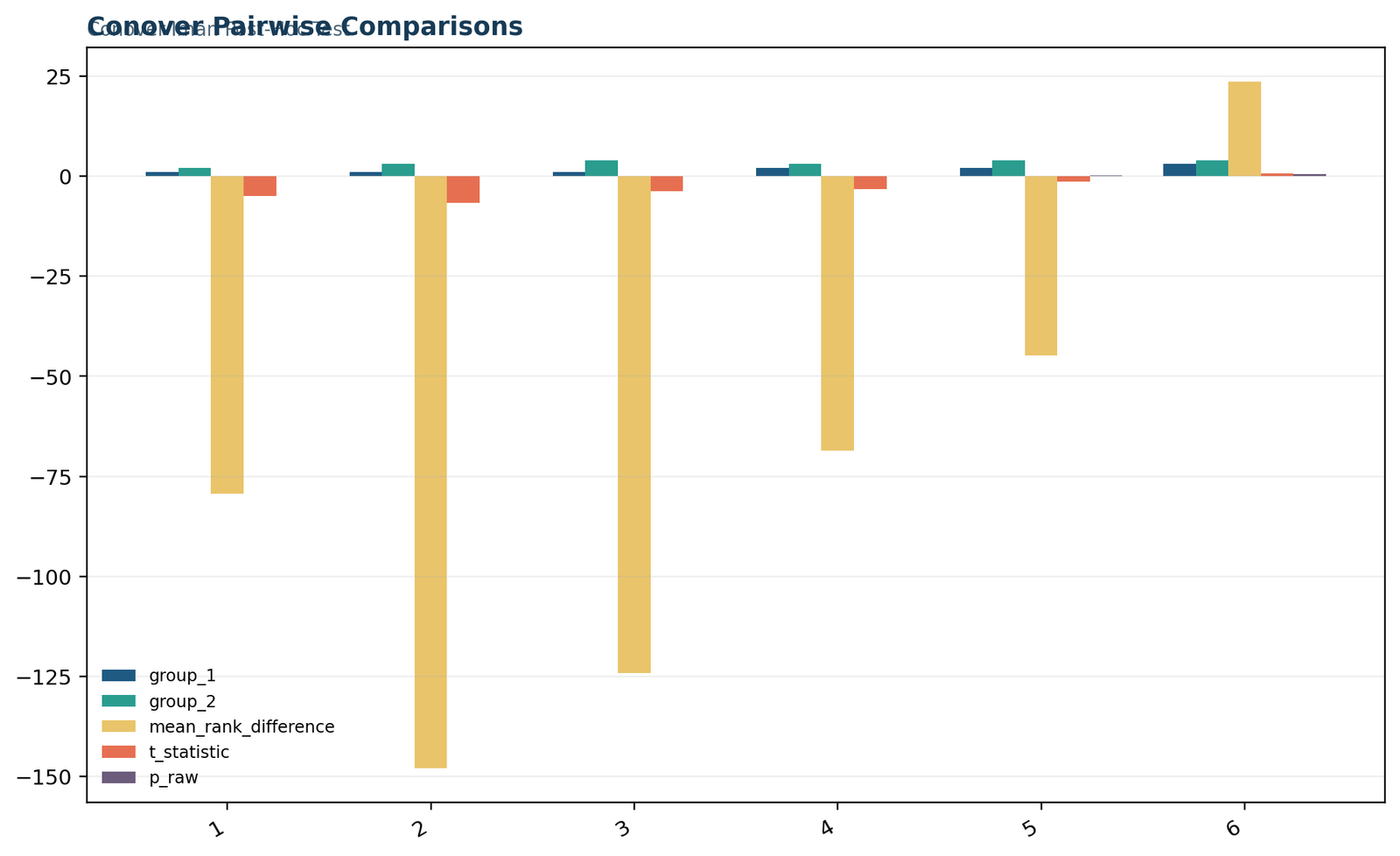
Pairwise Conover comparisons
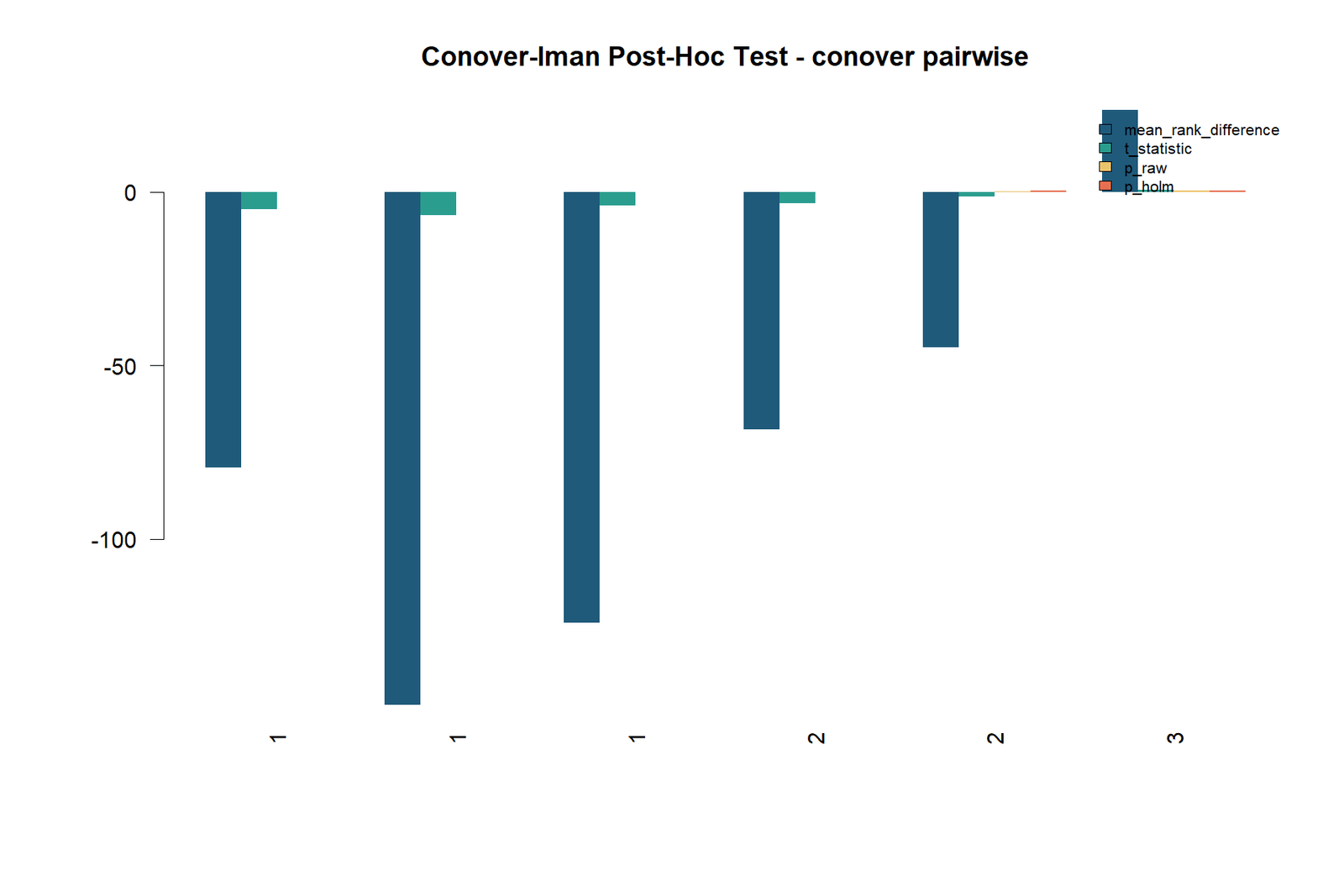
The largest standardized separation occurs for group 1 versus group 3: the mean-rank difference is −147.845 and the Conover statistic is t = −6.7256. The smallest separation is group 3 versus group 4, where the mean-rank difference is 23.629 and t = 0.6682. The chart therefore distinguishes the strong contrasts from pairs whose observed rank gaps are compatible with sampling variation.
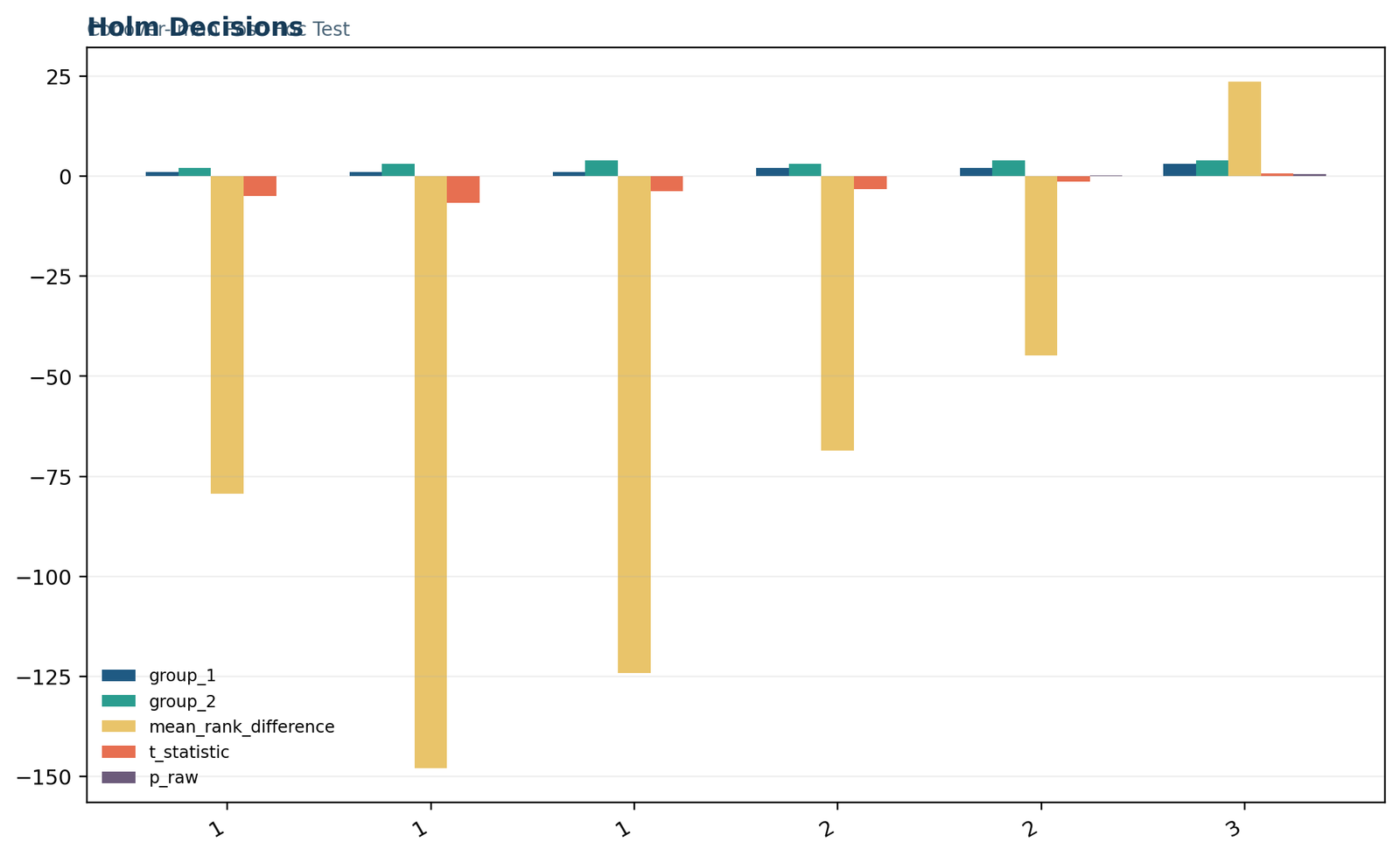
Holm-adjusted decisions
Four comparisons remain statistically significant after familywise-error control: 1 vs 2, 1 vs 3, 1 vs 4, and 2 vs 3. The 2 vs 4 comparison has Holm p = 0.322890, while 3 vs 4 has Holm p = 0.504222. The visual separates numerical rank differences from differences that remain statistically supported after adjustment.
Verified Python result summary
The final Python panel links the significant omnibus result to the exact post hoc pattern. Studytime group 1 differs from groups 2, 3, and 4, and group 2 differs from group 3; the remaining two pairs are not significant after Holm correction. This summary preserves the correct hierarchy from the Kruskal–Wallis finding to the Conover-Iman pairwise conclusions.
Conover test in R: conover.test and DescTools workflows
R offers dedicated implementations that return pairwise Conover-Iman comparisons and several p-value adjustments.
The Conover test in R can be performed with the conover.test package or DescTools::ConoverTest(). The two interfaces differ in output style, and group ordering plus adjustment labels form part of the result interpretation.
The R result can be compared with the same rank sums and mean ranks used in the Python analysis.
dat <- read.csv("dataset.csv")
dat$studytime <- factor(dat$studytime, levels = c(1, 2, 3, 4))# Omnibus stage
kruskal.test(G3 ~ studytime, data = dat)
# Conover-Iman with Holm correction
conover.test::conover.test(
x = dat$G3,
g = dat$studytime,
method = "holm",
kw = TRUE,
list = TRUE
)
# Alternative interface
DescTools::ConoverTest(G3 ~ studytime, data = dat, method = "holm")
R primary-metrics summary
The R analysis reproduces the central values from the independent calculation: H = 50.316208, p = 6.84157 × 10⁻¹¹, pooled rank variance s² = 34,704.863426, and minimum Holm p = 2.31527 × 10⁻¹⁰. The agreement establishes a common numerical foundation for the R, Python, SPSS-supported, and Excel interpretations.
R group rank profile
The R chart retains the same rank ordering: group 3 has the highest mean rank at 406.76, group 4 follows at 383.13, group 2 has 338.26, and group 1 has 258.91. The ordering shows that the principal distributional separation lies between the shortest study-time category and the higher study-time categories.
R pairwise comparison view
The signed contrasts preserve direction as well as significance. The negative differences for 1 vs 2, 1 vs 3, and 1 vs 4 indicate lower G3 ranks in group 1, while the −68.494 difference for 2 vs 3 indicates lower ranks in group 2. The positive 23.629 difference for 3 vs 4 is small relative to its standard error.
R Holm-adjusted decisions
The adjusted decision pattern matches the Python analysis. The four supported contrasts remain below α = .05 after Holm correction, whereas 2 vs 4 and 3 vs 4 remain above the decision threshold. Reporting the adjusted values preserves the familywise interpretation across all six comparisons.
Verified R result summary
The closing R panel condenses the omnibus result, the mean-rank ordering, and the Holm-adjusted pairwise decisions into one audit trail. Its substantive conclusion is identical to Python and Excel: four pairs differ significantly, with the largest separation between studytime groups 1 and 3.
Conover test in SPSS: omnibus ranks and pairwise computation
Base SPSS provides Kruskal-Wallis, pooled ranks and descriptives; the Conover-Iman pairwise stage requires custom computation or integrated Python/R.
The Conover test in SPSS workflow verifies data preparation, group mean ranks and the omnibus result before the pairwise Conover-Iman calculations are added through custom computation or integrated Python/R.
The Conover test is not exposed as a standard point-and-click SPSS pairwise table, so the custom calculation must be documented clearly.
What SPSS calculated directly
What requires custom calculation
Base SPSS supplies the pooled ranks, group summaries and Kruskal-Wallis statistic. The pairwise Conover-Iman stage additionally requires the pooled rank variance, pairwise standard errors, t statistics with df = N − k, raw two-sided p-values and a clearly named multiplicity adjustment.
These quantities can be calculated through embedded Python or R while retaining the native SPSS tables for the omnibus stage.
NPAR TESTS
/K-W = G3 BY studytime(1 4)
/STATISTICS = DESCRIPTIVES QUARTILES.RANK VARIABLES = G3 (A)
/RANK INTO conover_rank
/TIES = MEAN.
MEANS TABLES = conover_rank BY studytime
/CELLS = COUNT MEAN SUM STDDEV.
For general syntax and reporting guidance, see categorical data analysis in SPSS, ANOVA in SPSS, and t tests in SPSS.
Conover test in Excel: tie-corrected worked calculation
The workbook separates raw data, pooled ranks, formulas, diagnostics and reporting so every result can be audited.
The Conover test in Excel is not a single built-in command. A correct workbook must calculate pooled midranks, group rank sums, tie correction, H*, rank variance, pairwise standard errors, t statistics, raw p-values and Holm-adjusted decisions.
The Conover test workbook is strongest when every reported number can be traced back to a visible formula and a raw input cell.
Workbook architecture
Key Excel formulas
=RANK.AVG(G3_cell, all_G3_cells, 1)

=SUMIFS(rank_range, group_range, group_code)

=AVERAGEIFS(rank_range, group_range, group_code)

=T.DIST.2T(ABS(t_statistic), N-k)# Holm adjustment after sorting raw p-values

=MIN(1, raw_p * remaining_hypotheses)
Holm values must be monotone in sorted order. Helper columns or dynamic-array logic preserve monotone Holm values after the raw p-values are sorted.
How to interpret Conover test direction, magnitude and practical importance
Adjusted significance is only one part of the result; report rank direction, descriptive context and the omnibus effect.
A useful Conover test interpretation explains which group tends to have larger observations, how large the rank separation is, whether the result survives multiplicity correction, and whether the overall effect is practically meaningful.
Direction
The sign of the mean-rank difference identifies which listed group has lower ranks. For 1 vs 3, -147.845 means group 1 is lower than group 3.
Statistical strength
The adjusted p-value shows whether the pair remains significant after considering the six-test family. It does not measure effect size.
Practical context
Median G3 differs by two points between groups 1 and 3, while the omnibus epsilon squared is 0.073. The pattern is meaningful but not overwhelmingly large.
Omnibus effect size
The workbook reports epsilon squared = 0.07336. This summarizes the global strength of the association between studytime group and ranked final grade. It is an omnibus effect and does not belong to an individual Conover pair. Pairwise effect sizes require separate definitions and reporting.
Stochastic-dominance language
Some Conover documentation frames the pairwise null in terms of zero-order stochastic dominance. That interpretation is strongest when the empirical distribution functions do not cross in a way that reverses ordering. If the curves cross, report a general rank-distribution difference and show the underlying distributions rather than making an absolute “one group is better at every threshold” claim.
Related interpretation guides include effect size, p-values, confidence intervals, and Type I and Type II error.
Conover test vs Dunn, Nemenyi, Mann-Whitney and other methods
Method names are often treated as interchangeable online, but they use different statistics, assumptions and adjustment strategies.
The Conover test vs Dunn test comparison is the most common search intent. Both are post hoc rank procedures after Kruskal-Wallis, but the Conover-Iman statistic uses the pooled rank variance and the rejected omnibus signal with a t reference, often producing greater power.
| Method | Design and purpose | Reference statistic | When it is preferable | Main caution |
|---|---|---|---|---|
| Conover-Iman | Independent groups after significant Kruskal-Wallis | t on mean-rank differences, df = N-k | Powerful all-pairs follow-up with explicit p adjustment | Should be interpreted within the rejected omnibus framework |
| Dunn | Independent groups after Kruskal-Wallis | z-like standardized rank-sum difference | Very common, conservative and widely available | May have less power than Conover in some settings |
| Nemenyi | All-pairs rank comparisons | Studentized range | Balanced all-pairs settings and textbook comparisons | Can be conservative with unequal groups |
| DSCF | Dwass-Steel-Critchlow-Fligner pairwise test | Pairwise rank statistic | Direct nonparametric all-pairs inference | Different null calibration and software availability |
| Pairwise Mann-Whitney | Repeated two-group tests | U / rank-sum statistic | Simple exploratory follow-up with proper correction | Does not use the same omnibus-linked Conover variance |
| Tukey HSD | Parametric ANOVA post hoc | Studentized range on means | Normal, homoscedastic ANOVA model | Not a rank-based substitute when assumptions fail |
| Games-Howell | Parametric unequal-variance post hoc | Welch-type mean contrasts | Unequal variances and sample sizes with approximately normal means | Targets means, not rank distributions |
| Friedman-Conover | Repeated or blocked groups after Friedman | Blocked-rank comparison | Matched or repeated designs | Not valid for independent groups |
| Conover squared ranks | Test of dispersion or scale | Ranks of squared deviations | Variance-homogeneity question | Different test despite sharing the Conover name |
For parametric alternatives, compare one-way ANOVA, Welch’s ANOVA, Tukey HSD, Games-Howell, and pairwise comparisons after ANOVA.
Conover test diagnostics, sensitivity checks and common mistakes
A reliable post hoc analysis verifies the design, ranks, omnibus gate, p adjustment and reporting direction.
A complete Conover test report presents ties, factor labels, group sizes, distribution shape, omnibus significance and the adjustment method alongside the pairwise matrix.
Before running the test
After running the test
Ten frequent mistakes
- Running the Conover post hoc test after a non-significant Kruskal-Wallis result.
- Calling the procedure a direct test of group medians without checking shape.
- Using raw p-values when several pairs are tested.
- Reporting adjusted p-values without naming the adjustment.
- Ignoring the direction of the rank difference.
- Mixing independent-group Conover with Friedman-Conover syntax.
- Using inconsistent group ordering across software outputs.
- Omitting the tie correction when repeated outcome values are present.
- Interpreting non-significance as equivalence.
- Reporting H and p but omitting the exact significant pairs.
How to report the Conover test in APA style
Report the omnibus result first, then the adjustment method, significant pairs, non-significant pairs and descriptive direction.
An APA-style Conover test report is readable without the software output and includes the outcome and grouping variables, sample size, H statistic, degrees of freedom, omnibus p-value, adjustment, exact pairwise adjusted p-values and distribution-aware interpretation.
APA-style result
A Kruskal-Wallis test indicated that final grade differed across the four study-time groups, H(3) = 50.32, p < .001, ε² = .073. Conover-Iman post hoc comparisons with Holm adjustment showed that studytime group 1 had lower final-grade ranks than groups 2 (p = 4.78 × 10⁻⁶), 3 (p = 2.32 × 10⁻¹⁰) and 4 (p = .000642). Group 2 also had lower ranks than group 3 (p = .00332). The differences between groups 2 and 4 (p = .323) and between groups 3 and 4 (p = .504) were not significant.
Compact technical result
The tie-corrected Kruskal-Wallis statistic was H* = 50.3162 (df = 3, p = 6.84157 × 10⁻¹¹). Conover-Iman pairwise t tests used pooled rank variance s² = 34,704.8634 and df = 645. Four of six Holm-adjusted comparisons were significant.
Reporting checklist
State that groups are independent and identify the outcome and grouping variable.
Report H, df, exact or bounded p-value and an omnibus effect size.
Name Conover-Iman, the adjustment method and every pairwise decision.
Use mean ranks and descriptive summaries to explain which group tends higher.
Non-significant contrasts indicate insufficient evidence of a difference and are not evidence of equivalence.
Identify software, package, formula or workbook version used.
Conover test PDF, SPSS and Excel downloads
Open the exact reports and workbook used to verify the article results.
The downloadable Conover test PDF reports and worked Excel file provide the calculation trail behind every value in the article and allow the results to be reviewed across software platforms.
Python reportVerified omnibus metrics, group ranks, pairwise t statistics, raw p-values and Holm decisions.Open PDF →
R reportIndependent R replication of H, p, rank variance and the minimum Holm-adjusted p-value.Open PDF →
SPSS outputKruskal-Wallis tables, pooled ranks, group summaries and the test-specific verification block.Open PDF →
Worked Excel analysisRaw data, midranks, tie correction, formulas, diagnostics and reporting cross-checks.Open workbook →
Official Conover test references and software documentation
Primary software documentation used to verify the independent-groups post hoc procedure.
scikit-posthocs documentation
The official posthoc_conover documentation defines the Python interface, group/value arguments and p-adjustment options.
CRAN conover.test package
The CRAN conover.test page documents the Conover-Iman multiple-comparisons implementation and package materials.
DescTools ConoverTest
The official DescTools ConoverTest reference describes the Kruskal-Wallis follow-up, t statistic and interpretation conditions.
Conover test FAQs
Answers to the technical and search questions most often missed in shorter articles.
These Conover test FAQs cover the Conover-Iman name, Kruskal-Wallis requirement, differences from Dunn, software commands, ties, p-value adjustment, median interpretation and reporting.

