Normality Test, Estimated Parameters, Empirical CDF, D Statistic and SPSS Output
Lilliefors Test: Formula, Interpretation, SPSS, Python, R and Excel Guide
Lilliefors Test is a normality test used when the population mean and population standard deviation are unknown and estimated from the sample. This makes it more practical than the ordinary Kolmogorov-Smirnov Test for many real research datasets. In this complete guide, Salar Cafe explains the Lilliefors Test with formula, hypotheses, SPSS output interpretation, Python chart explanation, R validation charts, Excel workflow, APA reporting, common mistakes, downloadable resources, and internal links to related normality and assumption-testing guides.
Google AdSense top placement reserved here
Quick Answer: Lilliefors Test Result
The Lilliefors Test checks whether a sample follows a normal distribution when the normal distribution is fitted using the sample mean and sample standard deviation. This matters because in real projects, we usually do not know the true population mean and true population standard deviation. We estimate them from the data. The standard KS test assumes a fully specified reference distribution, while the Lilliefors version adjusts the normality-test logic for estimated parameters.
The null hypothesis says the sample comes from a normal distribution. The alternative hypothesis says the sample does not come from a normal distribution. If the p-value is less than .05, reject normality. If the p-value is greater than or equal to .05, do not reject normality. The test statistic is commonly written as D, the largest distance between the empirical CDF and the fitted normal CDF.
Final interpretation: The Lilliefors Test is the correct normality-test idea when the reference normal curve is fitted from the same sample. Report the D statistic, p-value, decision about normality, and supporting plots. A significant result means the sample distribution differs from the fitted normal distribution. A nonsignificant result means there is not enough evidence to reject normality, but it does not prove perfect normality.
Important reporting note: Use the Lilliefors result with visual checks such as a Q-Q plot normality check, P-P plot normality check, histogram interpretation, and box plot interpretation. Normality should not be judged by one p-value only.
Table of Contents
- What Is the Lilliefors Test?
- Why the Lilliefors Test Is Important
- Lilliefors Test Formula
- Null and Alternative Hypotheses
- Assumptions and Decision Logic
- Dataset and Variables Used
- Verified SPSS Output Interpretation
- Python Chart-by-Chart Interpretation
- R Chart-by-Chart Validation
- SPSS, Python, R and Excel Workflows
- SPSS, Python, R and Excel Code
- APA Reporting Wording
- Common Mistakes
- When to Use the Lilliefors Test
- Downloads and Resources
- Related Internal Guides
- FAQs
What Is the Lilliefors Test?
The Lilliefors Test is a normality test based on the Kolmogorov-Smirnov distance, but it is adjusted for the common situation where the mean and standard deviation of the normal reference distribution are estimated from the sample. That makes the Lilliefors Test very useful in student research, thesis analysis, SPSS normality tables, Python diagnostics, R normality workflows, and statistical consulting reports.
In the ordinary KS normality idea, the reference normal distribution must be fully specified in advance. In real analysis, that almost never happens. Instead, the analyst calculates the sample mean and sample standard deviation, fits a normal curve using those values, and compares the observed distribution with that fitted curve. The Lilliefors Test adjusts the p-value and decision rule for this estimated-parameter situation.
Simple definition: The Lilliefors Test checks whether sample data are normally distributed when the normal curve is fitted using the sample’s own mean and standard deviation.
Because it is a normality-test method, the Lilliefors Test belongs with other assumption-checking tools such as the D’Agostino-Pearson Test, Cramer-von Mises Test, Ryan-Joiner Test, Kolmogorov-Smirnov Test, and Q-Q Plot Normality Check 2.
Why the Lilliefors Test Is Important
The Lilliefors Test is important because many researchers incorrectly use a basic KS normality test even though the normal distribution parameters are estimated from the same data. This can lead to inaccurate interpretation. The Lilliefors version is specifically designed for the practical normality-checking situation in which the reference mean and standard deviation are not known before analysis.
For example, if a student checks whether final grades are normally distributed, the student normally calculates the sample mean and sample standard deviation from the grade data. The fitted normal curve then depends on the sample. The Lilliefors Test accounts for that dependency. That is why it is often discussed as a corrected or adjusted KS-style normality test.
| Feature | Ordinary KS Normality Use | Lilliefors Test | Practical Meaning |
|---|---|---|---|
| Reference distribution | Fully specified in advance | Fitted from sample mean and sample SD | Lilliefors fits real research situations better. |
| Mean and SD | Known before testing | Estimated from the sample | Most research datasets require estimation. |
| Purpose | General distribution fit | Normality with estimated parameters | Lilliefors is more targeted for normality diagnostics. |
| Interpretation | Compare ECDF to fixed CDF | Compare ECDF to fitted normal CDF | The p-value logic changes because parameters are estimated. |
When reporting a normality assumption, use the Lilliefors Test with supporting descriptive tools such as descriptive statistics, frequency distribution, five-number summary, and coefficient of variation.
Lilliefors Test Formula
The Lilliefors Test uses the largest absolute gap between the empirical cumulative distribution function and the fitted normal cumulative distribution function.
Where:
| Symbol | Meaning | Interpretation |
|---|---|---|
| D | Lilliefors D statistic | The largest distance between observed ECDF and fitted normal CDF. |
| Fn(x) | Empirical CDF | The observed cumulative proportion at or below x. |
| Φ | Standard normal CDF | The theoretical cumulative probability after standardization. |
| x̄ | Sample mean | Estimated from the same sample being tested. |
| s | Sample standard deviation | Estimated from the same sample being tested. |
D Plus and D Minus
The D statistic can also be explained using two directional gaps. D plus shows where the empirical CDF is above the fitted normal CDF. D minus shows where the fitted normal CDF is above the empirical CDF. The final Lilliefors D statistic is the larger absolute gap.
Formula caution: The Lilliefors D statistic resembles the KS D statistic, but the p-value is different because the normal mean and standard deviation are estimated from the sample. This is the main reason the Lilliefors Test is not identical to the ordinary Kolmogorov-Smirnov Test.
Null and Alternative Hypotheses for the Lilliefors Test
The Lilliefors Test is a formal normality test, so the null and alternative hypotheses should be written clearly before interpreting output.
| Hypothesis | Statement | Meaning for Reporting |
|---|---|---|
| Null hypothesis | H0: The sample data come from a normal distribution. | Normality is acceptable under the test. |
| Alternative hypothesis | H1: The sample data do not come from a normal distribution. | The normality assumption is not supported. |
| Decision rule | Reject H0 if p < .05. | A significant p-value indicates non-normality. |
Decision wording: If the Lilliefors p-value is below .05, write that the distribution differs significantly from normal. If the p-value is not below .05, write that the test did not provide sufficient evidence to reject normality.
The hypothesis decision is especially important before parametric methods such as a one-tailed t test, one-sample z test, confidence interval, regression diagnostics such as the Ramsey RESET Test, and assumption checks such as the Levene Test.
Assumptions and Decision Logic
The Lilliefors Test is itself an assumption-checking tool, but it still requires careful interpretation. The observations should be independent, the variable should be numeric, and the test should be interpreted with visual evidence rather than as an isolated p-value.
| Requirement | Why It Matters | What to Do |
|---|---|---|
| Numeric variable | The test compares cumulative numeric distributions. | Use continuous or approximately continuous variables where possible. |
| Independent observations | Repeated or dependent observations can distort normality interpretation. | Check study design before testing. |
| Estimated mean and SD | This is the reason for using Lilliefors instead of ordinary KS normality logic. | Use the Lilliefors p-value or corrected method. |
| Visual confirmation | Large samples can make tiny deviations significant. | Use histogram, Q-Q plot, P-P plot and ECDF plots. |
For repeated-measures or variance assumption contexts, use separate assumption checks such as Mauchly’s Test of Sphericity, Greenhouse-Geisser Correction, Cochran C Test, and Brown-Forsythe Test.
Dataset and Variables Used
The worked Lilliefors Test example uses student performance variables. The main chart set focuses on normality diagnostics for a numeric variable such as G3 final grade, while the cross-variable charts compare Lilliefors D statistics across several numeric variables. This helps show that normality is variable-specific. One variable can look close to normal while another variable can be highly skewed.
| Dataset Element | Role in the Lilliefors Test | Why It Matters |
|---|---|---|
| Main numeric variable | Primary normality test variable | Used for distribution fit and ECDF comparison. |
| Sample mean | Estimated normal parameter | Used to fit the normal reference curve. |
| Sample standard deviation | Estimated normal parameter | Used to scale the fitted normal CDF. |
| Empirical CDF | Observed cumulative distribution | Compared with the fitted normal CDF to calculate D. |
| Multiple numeric variables | Cross-variable comparison | Shows which variables depart more strongly from normality. |
| Group variable | Group diagnostic comparison | Shows whether normality differs across subgroups. |
Before running the Lilliefors Test, it is good practice to examine descriptive statistics, frequency distributions, histograms, box plots, and five-number summaries.
Google AdSense middle placement reserved here
Verified SPSS Output Interpretation
The SPSS output PDF supports the Lilliefors Test normality workflow for this post. In SPSS-style interpretation, the analyst should report the normality-test statistic, significance value, decision about the null hypothesis, and supporting graphical evidence. Because the Lilliefors Test is connected to KS-style normality testing with estimated parameters, the interpretation should be precise and not confused with a fully specified ordinary KS test.
How to Read the SPSS Output
| SPSS Output Item | What It Means | How to Interpret |
|---|---|---|
| Test statistic | The Lilliefors/KS-style D statistic | Larger D means a larger gap between the empirical distribution and fitted normal distribution. |
| Significance value | p-value | If p < .05, reject normality. |
| Histogram | Shape of observed distribution | Explains whether skewness, tails, peaks or outliers influence the test. |
| Normality plots | Q-Q or P-P visual diagnostics | Show whether points follow the expected normal pattern. |
| Descriptive statistics | Mean, standard deviation, skewness, kurtosis | Provide context for the test decision. |
SPSS Decision Logic
If the SPSS p-value is below .05, write that the Lilliefors Test indicated a statistically significant departure from normality. If the p-value is above .05, write that the test did not find sufficient evidence to reject normality. Do not write that the data are “perfectly normal.” A nonsignificant result only means the evidence against normality is not strong enough under this test.
SPSS conclusion template: The Lilliefors normality result should be interpreted as a distribution-fit decision. The D statistic shows the maximum ECDF-to-fitted-CDF distance, while the p-value indicates whether the distance is statistically large enough to reject normality. The final conclusion should be supported with histogram, ECDF, Q-Q plot, or P-P plot evidence.
SPSS reporting caution: SPSS normality outputs may describe the result in KS-style terms. When the normal curve is fitted from the sample mean and standard deviation, explain that the interpretation is Lilliefors-style or based on estimated normal parameters.
Python Chart-by-Chart Interpretation
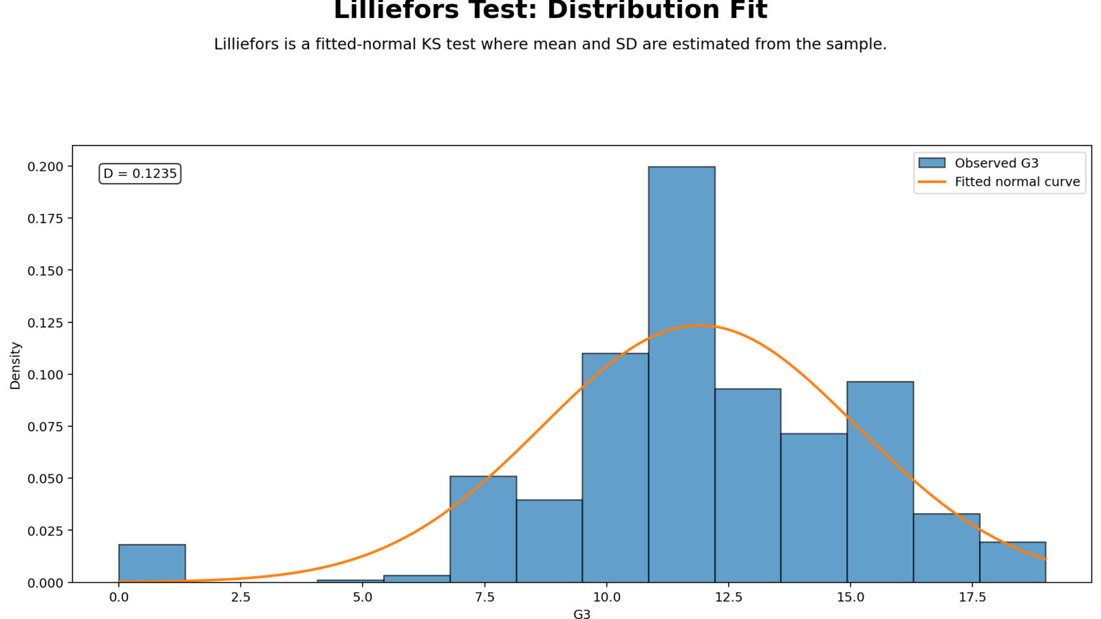
The provided Python output contains one distribution-fit chart for the Lilliefors Test. This chart is still important because it shows the practical visual comparison that motivates the test: observed data shape versus fitted normal shape.
Python Chart 1: Distribution Fit for Lilliefors Test
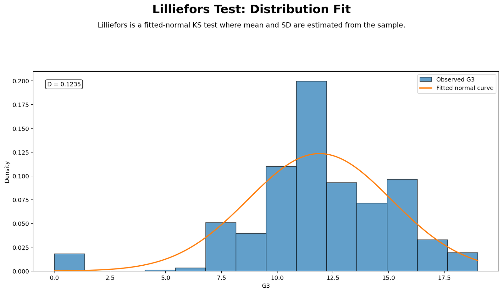
This Python chart shows how the sample distribution compares with the fitted normal distribution. The fitted normal curve is based on the sample mean and sample standard deviation, which is exactly why the Lilliefors Test is needed. If the histogram or density shape follows the normal reference curve closely, the normality assumption becomes more plausible. If the observed distribution is skewed, heavy-tailed, too peaked, too flat, or irregular, the Lilliefors D statistic becomes larger.
The chart is useful because the p-value alone does not explain the pattern of non-normality. A significant result may be caused by skewness, outliers, kurtosis, floor effects, ceiling effects, or distribution gaps. This chart gives the visual reason behind the test decision. In a full normality workflow, this figure should be read together with the Q-Q plot normality check and P-P plot normality check.
Decision/reporting conclusion: Use this Python chart to support the Lilliefors normality decision. If the observed distribution visibly departs from the fitted normal curve, report that the chart supports non-normality. If the fit is close, report that the visual evidence supports approximate normality, while still using the p-value for the formal decision.
R Chart-by-Chart Validation
The R charts provide a complete validation workflow for the Lilliefors Test. They show the distribution fit, empirical CDF comparison, D plus and D minus gaps, Monte Carlo reference distribution, p-value decision, D statistic across variables, and group comparison.
R Chart 1: Distribution Fit for Lilliefors Test
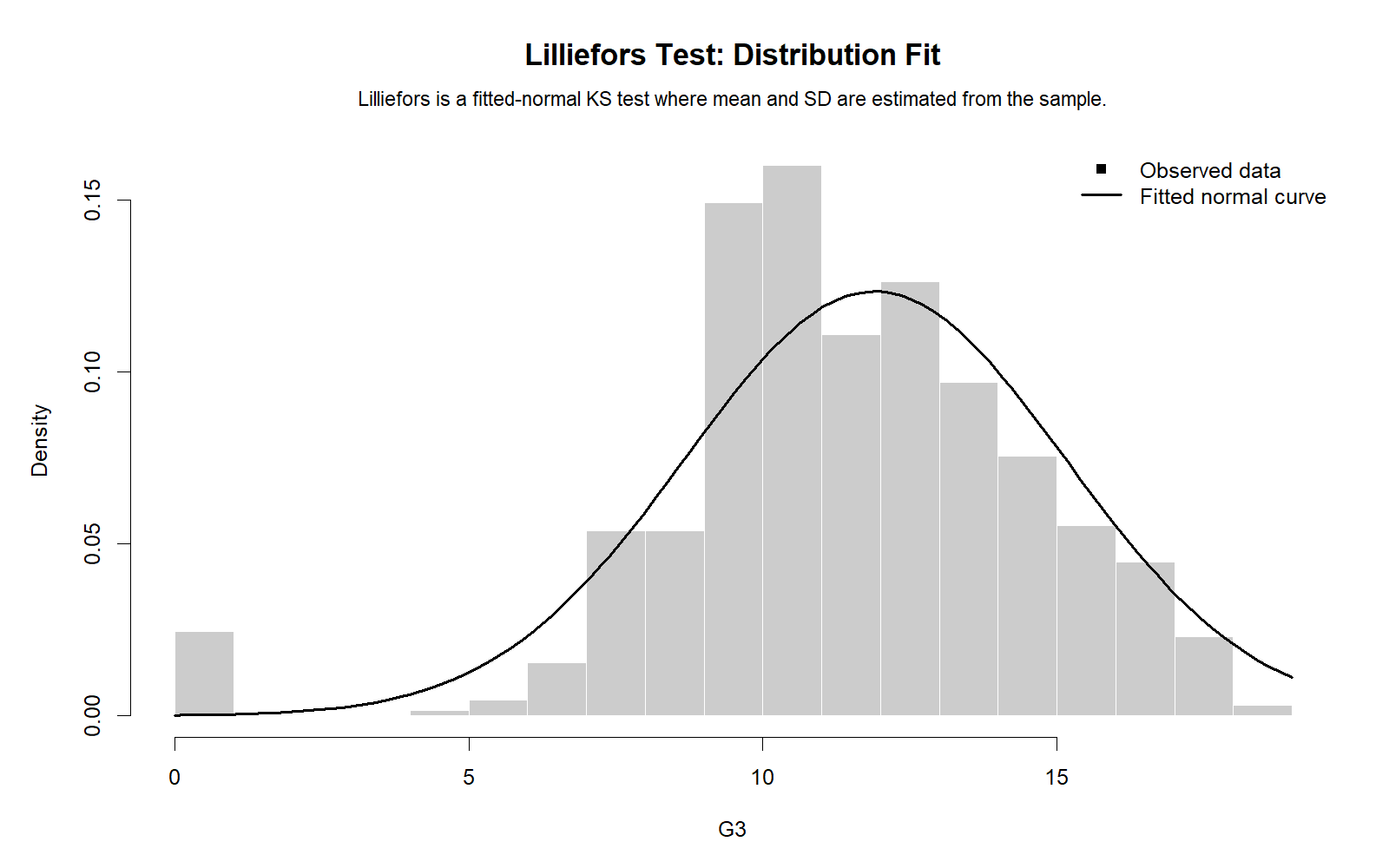
This R chart validates the Python distribution-fit result. It compares the observed data distribution with the fitted normal reference. If the observed bars or density shape are close to the normal curve, the Lilliefors D statistic should be smaller. If the distribution has skewness, heavy tails, or unusual clustering, the D statistic becomes larger.
Decision/reporting conclusion: This chart should be used as the first visual support for the Lilliefors decision. It tells the reader whether the formal result is visually reasonable.
R Chart 2: Empirical CDF vs Fitted Normal CDF
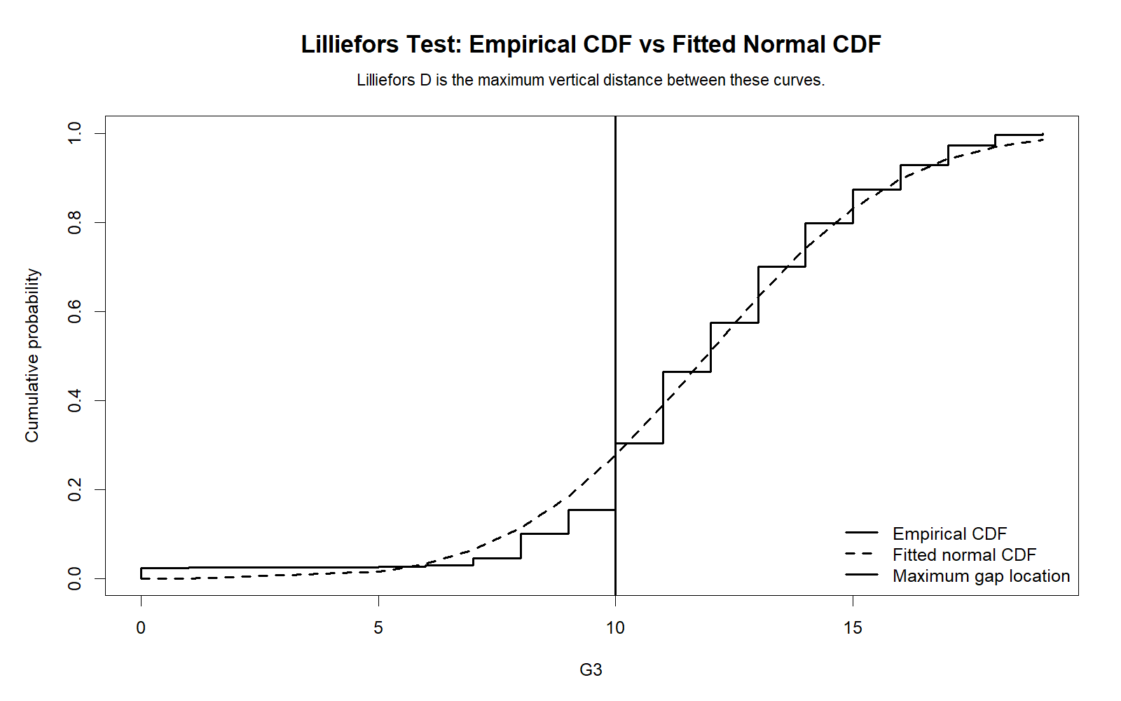
This is the most important conceptual chart for the Lilliefors Test. The empirical CDF shows the cumulative pattern of the observed sample. The fitted normal CDF shows the expected cumulative pattern if the sample were normally distributed with the sample’s estimated mean and standard deviation. The Lilliefors D statistic is based on the largest vertical separation between these two curves.
If the two curves stay close together, the data are closer to normal. If the curves separate strongly in the middle, lower tail, or upper tail, the evidence against normality becomes stronger. This chart explains the test more clearly than a table alone.
Decision/reporting conclusion: Use this ECDF chart to explain where the empirical distribution differs most from the fitted normal distribution. The largest visible vertical gap is the core evidence behind the Lilliefors statistic.
R Chart 3: D Plus and D Minus Gaps
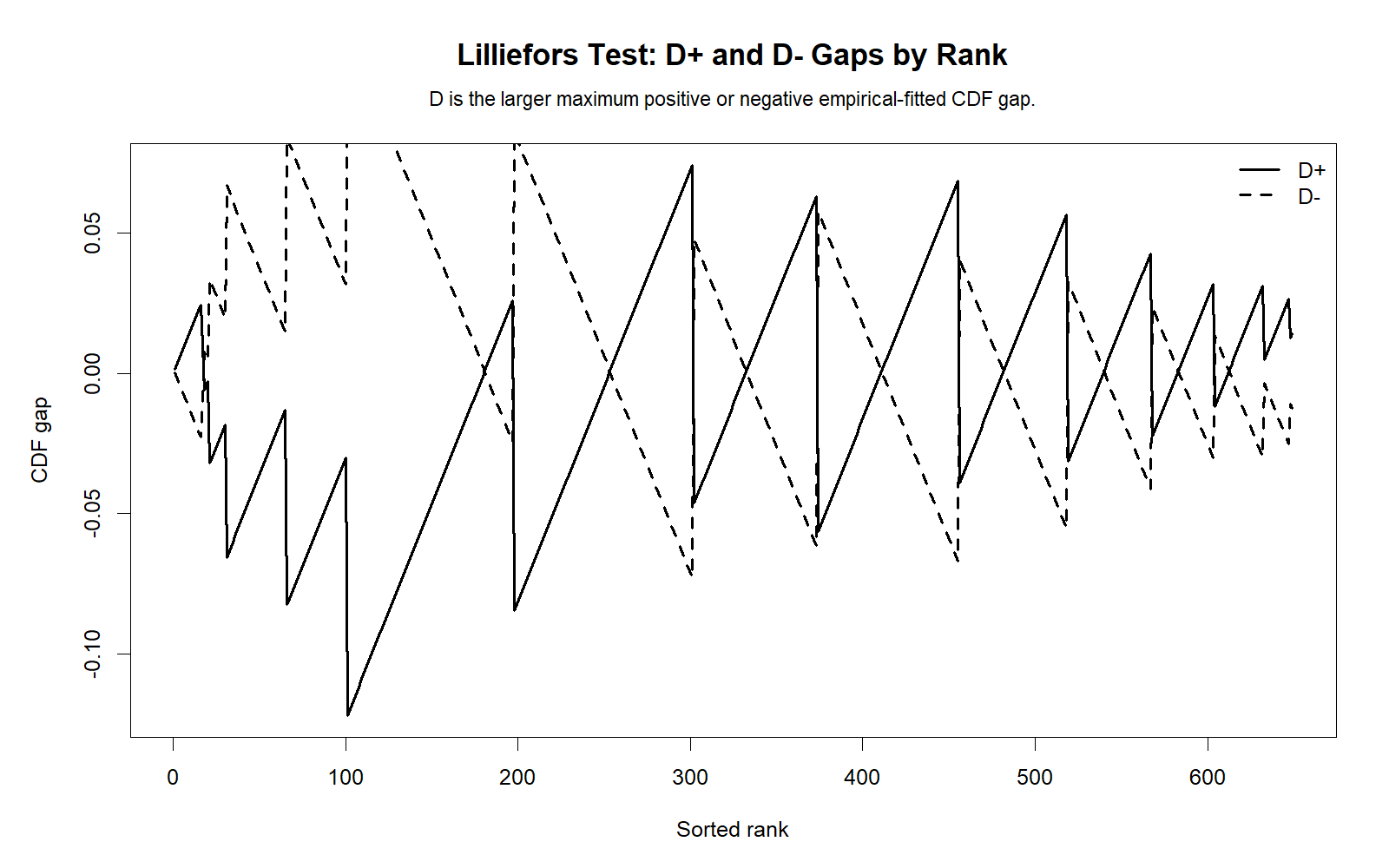
This chart shows the directional gaps behind the Lilliefors statistic. D plus occurs when the empirical CDF is above the fitted normal CDF. D minus occurs when the fitted normal CDF is above the empirical CDF. The final D statistic is the larger absolute gap.
This figure is useful for teaching and reporting because it shows the exact area where the data depart most strongly from normality. Instead of only saying that D is large or small, the chart shows the location and direction of the maximum discrepancy.
Decision/reporting conclusion: Use this chart to justify the D statistic and to describe whether the strongest departure is in the lower tail, center, or upper tail of the distribution.
R Chart 4: Monte Carlo Reference Distribution
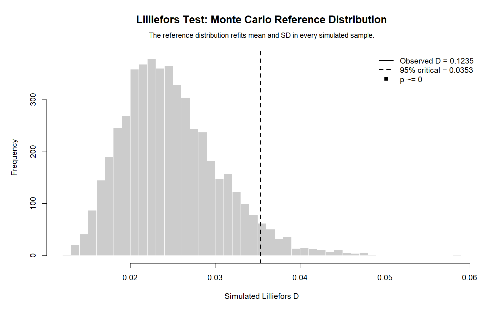
The Lilliefors Test requires special p-value logic because the normal mean and standard deviation are estimated from the data. A Monte Carlo reference distribution shows what D values are expected when samples are drawn from a normal distribution and parameters are estimated in the same way.
If the observed D statistic is far into the extreme tail of this simulated reference distribution, the p-value becomes small and the normality assumption is rejected. This chart makes the p-value visually understandable.
Decision/reporting conclusion: Use this chart to explain whether the observed D statistic is typical or unusual under the fitted-normal null model.
R Chart 5: P-value Decision
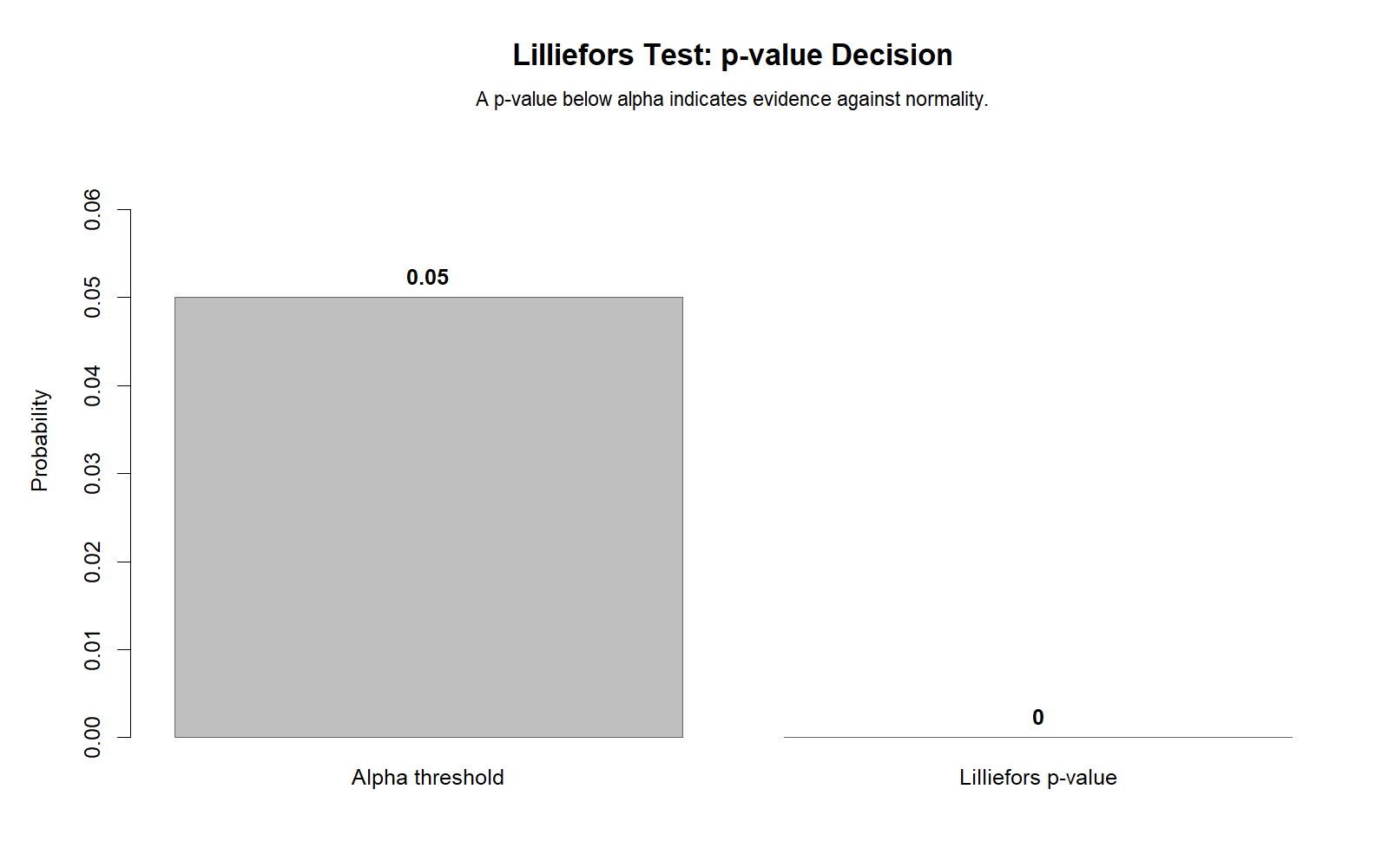
This chart presents the final test decision in a simple visual form. If the p-value is below .05, the Lilliefors result is statistically significant and normality is rejected. If the p-value is greater than or equal to .05, normality is not rejected.
The p-value decision is useful for quick reporting, but it should be interpreted with the distribution-fit chart and ECDF chart. A p-value tells whether the difference is statistically meaningful; the charts tell what the difference looks like.
Decision/reporting conclusion: Use this p-value chart as the final decision aid, but do not report it without the supporting visual evidence.
R Chart 6: Lilliefors D Across Variables
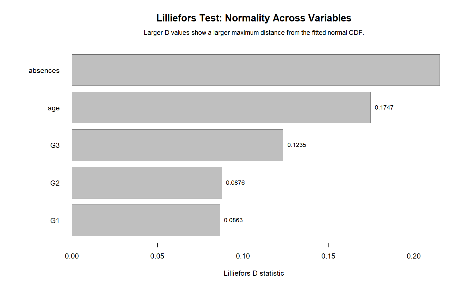
This chart compares Lilliefors D values across different numeric variables. A larger D statistic indicates a stronger departure from the fitted normal distribution. This is useful because normality is not a property of the entire dataset; it must be assessed for the specific variable or residual series relevant to the analysis.
For example, a grade variable may show a different normality pattern than a count variable such as absences. A count variable may require a transformation such as reciprocal transformation, a square-root transformation, or a nonparametric approach.
Decision/reporting conclusion: Use this chart to identify which variables need closer normality review, transformation, robust analysis, or nonparametric methods.
R Chart 7: Group Lilliefors D Comparison
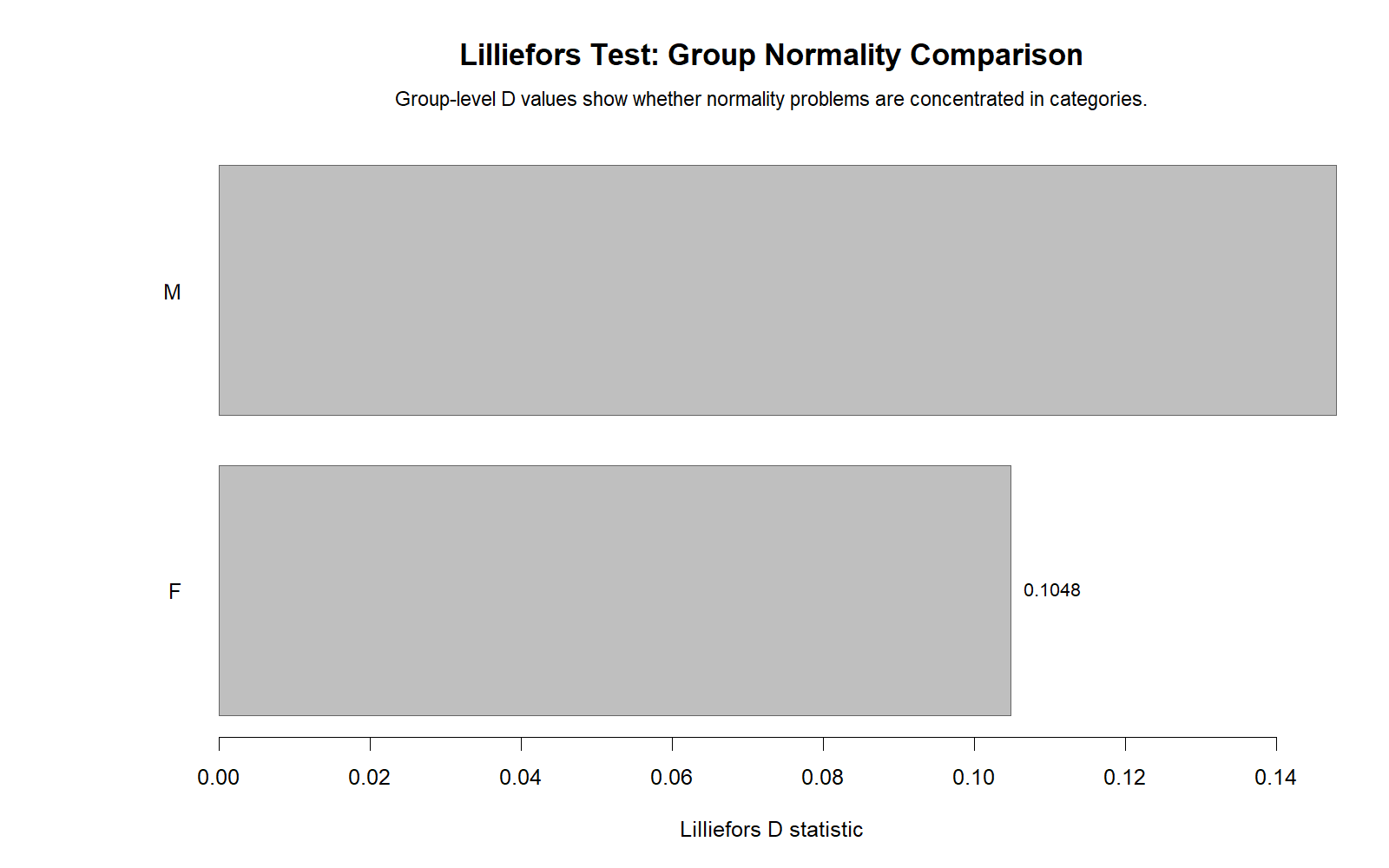
This chart compares the strength of non-normality across groups. A variable may look approximately normal in one subgroup but non-normal in another. This is important when the next analysis compares groups, such as a t test, ANOVA, or group-based regression model.
Group-specific normality checks should be interpreted with variance assumptions too. For example, if a group comparison is planned, pair the Lilliefors normality decision with variance checks such as the Levene Test, Brown-Forsythe Test, or Cochran C Test.
Decision/reporting conclusion: Use this chart to decide whether normality problems are general or concentrated in particular groups. This helps choose between parametric, robust, transformed, or nonparametric analysis.
Google AdSense in-content placement reserved here
SPSS, Python, R and Excel Workflows for the Lilliefors Test
A complete Lilliefors Test workflow should not stop at one p-value. The best workflow includes descriptive statistics, fitted normal comparison, ECDF diagnostics, D statistic, p-value, and a final reporting decision. This workflow is useful before parametric tests, confidence interval estimation, regression modeling, cross tabulation reporting for categorical summaries, and broader data-quality review.
SPSS Workflow
| Step | SPSS Action | Purpose |
|---|---|---|
| Open data | File > Open > Data | Load the SPSS-ready dataset. |
| Explore variable | Analyze > Descriptive Statistics > Explore | Request descriptives, histogram, and normality plots. |
| Read normality table | Tests of Normality output | Identify D statistic and p-value. |
| Inspect plots | Histogram, Q-Q plot, P-P plot | Explain the source of normality departure. |
| Report result | APA statement | State whether normality is rejected or not rejected. |
Python Workflow
| Step | Python Action | Purpose |
|---|---|---|
| Read dataset | pandas.read_csv() | Load data into Python. |
| Select variable | pd.to_numeric() and dropna() | Prepare clean numeric data. |
| Run Lilliefors | statsmodels.stats.diagnostic.lilliefors() | Get D statistic and p-value. |
| Plot fitted distribution | matplotlib | Compare observed shape with fitted normal curve. |
| Interpret | p-value and chart evidence | Decide whether normality is supported. |
R Workflow
| Step | R Action | Purpose |
|---|---|---|
| Read data | read.csv() | Import dataset. |
| Select variable | na.omit() | Remove missing values. |
| Run test | nortest::lillie.test() | Calculate the Lilliefors result. |
| Create ECDF | ecdf() or manual ECDF | Visualize observed cumulative distribution. |
| Plot diagnostics | Base R or ggplot2 | Create distribution, ECDF, D gap, and p-value decision charts. |
Excel Workflow
| Excel Task | Formula or Method | Purpose |
|---|---|---|
| Sort values | Sort smallest to largest | Create ordered values for ECDF. |
| Mean | =AVERAGE(range) | Estimate normal mean. |
| Standard deviation | =STDEV.S(range) | Estimate normal standard deviation. |
| Empirical CDF | =rank/n | Calculate observed cumulative probabilities. |
| Fitted normal CDF | =NORM.DIST(x,mean,sd,TRUE) | Calculate fitted normal cumulative probabilities. |
| D statistic | =MAX(ABS(empirical-normal)) | Find the largest ECDF-CDF gap. |
SPSS, Python, R and Excel Code for the Lilliefors Test
SPSS Syntax for Lilliefors Normality Workflow
* Lilliefors-style normality workflow in SPSS.
* Replace G3 with your selected numeric variable.

TITLE "Lilliefors Test Normality Workflow".

EXAMINE VARIABLES=G3
  /PLOT BOXPLOT HISTOGRAM NPPLOT
  /COMPARE GROUPS
  /STATISTICS DESCRIPTIVES
  /CINTERVAL 95
  /MISSING LISTWISE
  /NOTOTAL.

NPAR TESTS
  /K-S(NORMAL)=G3
  /MISSING ANALYSIS.

FREQUENCIES VARIABLES=G3
  /STATISTICS=MEAN MEDIAN STDDEV SKEWNESS SESKEW KURTOSIS SEKURT MINIMUM MAXIMUM
  /HISTOGRAM NORMAL
  /ORDER=ANALYSIS.

OUTPUT EXPORT
  /CONTENTS EXPORT=VISIBLE
  /PDF DOCUMENTFILE="Lilliefors-Test-SPSS-Output.pdf".
Python Code for the Lilliefors Test
import pandas as pd
import numpy as np
import matplotlib.pyplot as plt
from scipy.stats import norm
from statsmodels.stats.diagnostic import lilliefors

df = pd.read_csv("dataset.csv")

x = pd.to_numeric(df["G3"], errors="coerce").dropna().to_numpy()

# Lilliefors test for normality
d_stat, p_value = lilliefors(x, dist="norm")

print("Lilliefors D statistic:", d_stat)
print("p-value:", p_value)

if p_value < 0.05:
    print("Reject normality")
else:
    print("Do not reject normality")

# Fitted normal parameters
mu = np.mean(x)
sigma = np.std(x, ddof=1)

# Empirical CDF and fitted normal CDF
x_sorted = np.sort(x)
n = len(x_sorted)
ecdf = np.arange(1, n + 1) / n
fitted_cdf = norm.cdf(x_sorted, loc=mu, scale=sigma)

# D statistic manually
abs_gap = np.abs(ecdf - fitted_cdf)
manual_d = np.max(abs_gap)

print("Manual maximum gap:", manual_d)

# Plot ECDF and fitted CDF
plt.figure(figsize=(8, 5))
plt.step(x_sorted, ecdf, where="post", label="Empirical CDF")
plt.plot(x_sorted, fitted_cdf, label="Fitted Normal CDF")
plt.title("Lilliefors Test: Empirical CDF vs Fitted Normal CDF")
plt.xlabel("Observed value")
plt.ylabel("Cumulative probability")
plt.legend()
plt.tight_layout()
plt.show()
R Code for the Lilliefors Test
# Lilliefors Test in R

# install.packages("nortest")
library(nortest)

df <- read.csv("dataset.csv")

x <- as.numeric(df$G3)
x <- na.omit(x)

# Run Lilliefors Test
result <- lillie.test(x)
print(result)

# Estimate normal parameters
mu <- mean(x)
sigma <- sd(x)

# Create ECDF and fitted normal CDF
x_sorted <- sort(x)
n <- length(x_sorted)
ecdf_vals <- (1:n) / n
fitted_cdf <- pnorm(x_sorted, mean = mu, sd = sigma)

# Maximum gap
gap <- abs(ecdf_vals - fitted_cdf)
D_manual <- max(gap)

print(D_manual)

# Plot
plot(x_sorted, ecdf_vals, type = "s",
     main = "Lilliefors Test: ECDF vs Fitted Normal CDF",
     xlab = "Observed value",
     ylab = "Cumulative probability")
lines(x_sorted, fitted_cdf, col = "blue", lwd = 2)
legend("bottomright",
       legend = c("Empirical CDF", "Fitted Normal CDF"),
       col = c("black", "blue"),
       lwd = c(1, 2),
       bty = "n")
Excel Formulas for a Lilliefors-Style Manual Check
Assume sorted values are in A2:A650.

Sample size:
=COUNT(A2:A650)

Mean:
=AVERAGE(A2:A650)

Standard deviation:
=STDEV.S(A2:A650)

Rank position in B2:
=ROW(A1)

Empirical CDF in C2:
=B2/COUNT($A$2:$A$650)

Fitted normal CDF in D2:
=NORM.DIST(A2,$Mean_Cell$,$SD_Cell$,TRUE)

Absolute gap in E2:
=ABS(C2-D2)

Lilliefors-style D statistic:
=MAX(E2:E650)

Decision:
Use SPSS, R, or Python for the formal Lilliefors p-value.
Use Excel mainly to understand and visualize the ECDF-CDF gap.
APA Reporting Wording for the Lilliefors Test
APA reporting for the Lilliefors Test should include the variable, D statistic, p-value, hypothesis decision, and a short interpretation. A strong report should also mention supporting visual evidence such as the histogram, ECDF chart, Q-Q plot, or P-P plot.
If the Lilliefors Test Is Significant
The Lilliefors Test indicated that the distribution departed significantly from normality, D = [value], p < .05. Therefore, the null hypothesis of normality was rejected. Visual inspection of the distribution and cumulative distribution plots supported this conclusion.
If the Lilliefors Test Is Not Significant
The Lilliefors Test was not significant, D = [value], p ≥ .05. Therefore, the test did not provide sufficient evidence to reject the normality assumption. The distribution was also reviewed using graphical diagnostics before the final decision was made.
Student-Friendly Report Sentence
The Lilliefors Test was used because the normal distribution parameters were estimated from the sample. The result was interpreted using the p-value and visual plots. This approach is more appropriate than relying on an ordinary KS test when the population mean and standard deviation are not known in advance.
Common Mistakes in Lilliefors Test Interpretation
| Mistake | Why It Is a Problem | Correct Practice |
|---|---|---|
| Confusing Lilliefors with ordinary KS | Ordinary KS assumes known parameters; Lilliefors handles estimated parameters. | Use Lilliefors wording when mean and SD are estimated from the sample. |
| Reporting only the p-value | The p-value does not show the shape of non-normality. | Use histogram, ECDF, Q-Q plot, and P-P plot evidence. |
| Saying nonsignificant means perfectly normal | Failure to reject normality is not proof of perfect normality. | Write “did not provide evidence against normality.” |
| Ignoring sample size | Large samples can make small deviations significant. | Interpret p-value with practical visual shape. |
| Testing the wrong variable | Normality should match the analysis target, often residuals rather than raw outcomes. | Check the variable or residuals relevant to the planned method. |
| Skipping follow-up decisions | Normality results should guide analysis choice. | Consider transformation, robust methods, nonparametric tests, or the Central Limit Theorem. |
Key reminder: The Lilliefors Test is one part of a full assumption-checking workflow. It should be interpreted together with related tools such as D’Agostino-Pearson Test, Cramer-von Mises Test, and Ryan-Joiner Test.
When to Use the Lilliefors Test
Use the Lilliefors Test when you need a normality test and the population mean and standard deviation are unknown. That is the normal situation in most real research datasets. It is especially useful before parametric tests, regression modeling, confidence interval reporting, or any analysis where normality is part of the assumption discussion.
| Use the Lilliefors Test When | Reason | Related Guide |
|---|---|---|
| Mean and SD are estimated from the sample | This is the main reason Lilliefors is needed. | Kolmogorov-Smirnov Test |
| You are checking normality before a parametric method | Normality affects interpretation of many statistical tests. | One-Tailed T Test |
| You need visual evidence of distribution fit | ECDF and fitted CDF explain the D statistic. | Q-Q Plot Normality Check |
| You are comparing several variables | D across variables shows which variables deviate more from normality. | Descriptive Statistics |
| You need a complete assumption report | Normality should be reported with other assumptions. | Levene Test |
If the Lilliefors Test rejects normality, do not panic automatically. Review sample size, plot shape, outliers, skewness, kurtosis, and the planned method. In some situations, transformation, robust methods, bootstrapping, or effect-size reporting may be more useful than forcing the data to look perfectly normal. For reporting strength, connect the normality result with effect size, confidence interval, and visual diagnostics.
Downloads and Resources for the Lilliefors Test
The SPSS output PDF below supports the Lilliefors Test workflow used in this guide. The chart URLs also provide the visual diagnostic evidence for distribution fit, ECDF comparison, D gaps, Monte Carlo reference distribution, p-value decision, variable comparison, and group comparison.
Download SPSS Output PDF
Verified SPSS output for the Lilliefors Test normality workflow.
Copy Lilliefors Test Code
Use the SPSS, Python, R and Excel code blocks to reproduce the analysis.
Python Distribution Fit Chart
Visual comparison of sample distribution and fitted normal reference.
R ECDF vs Fitted Normal CDF Chart
Main visual explanation of the Lilliefors D statistic.
FAQs About the Lilliefors Test
What is the Lilliefors Test?
The Lilliefors Test is a normality test used when the mean and standard deviation of the normal reference distribution are estimated from the sample.
What is the Lilliefors Test used for?
It is used to check whether a numeric sample variable follows a normal distribution when population parameters are unknown.
Is the Lilliefors Test the same as the Kolmogorov-Smirnov Test?
No. It is related to the KS test, but it adjusts the normality-test logic for estimated sample mean and standard deviation.
What is the null hypothesis of the Lilliefors Test?
The null hypothesis says that the sample data come from a normal distribution.
What is the alternative hypothesis of the Lilliefors Test?
The alternative hypothesis says that the sample data do not come from a normal distribution.
What does the Lilliefors D statistic mean?
The D statistic is the largest distance between the empirical CDF and the fitted normal CDF.
How do I interpret a significant Lilliefors Test?
If p < .05, reject normality and conclude that the sample distribution differs significantly from the fitted normal distribution.
How do I interpret a nonsignificant Lilliefors Test?
If p ≥ .05, do not reject normality. This means the test did not find enough evidence against normality, not that the data are perfectly normal.
Can I run the Lilliefors Test in SPSS?
SPSS supports normality-testing workflows through Explore and KS-style outputs. Interpret them carefully when parameters are estimated from the sample.
Can I run the Lilliefors Test in Python?
Yes. Python can run the Lilliefors Test using statsmodels.stats.diagnostic.lilliefors().
Can I run the Lilliefors Test in R?
Yes. R can run the Lilliefors Test using nortest::lillie.test().
Can I calculate the Lilliefors Test in Excel?
Excel can calculate the ECDF, fitted normal CDF, and D statistic manually, but SPSS, Python, or R should be used for a formal p-value.
Should I use charts with the Lilliefors Test?
Yes. Use histogram, ECDF, Q-Q plot, and P-P plot evidence to explain the normality decision.
What should I do if the Lilliefors Test rejects normality?
Review the plots, sample size, outliers, skewness, kurtosis, and planned method. Consider transformation, robust methods, nonparametric tests, or Central Limit Theorem reasoning where appropriate.
Google AdSense bottom placement reserved here