
Mixed Effects Regression: Formula, Interpretation, SPSS, Python, R and Excel Guide
Mixed Effects Regression is used when observations are grouped or repeatedly measured. This beginner-friendly example follows 649 students across G1, G2 and G3, creates 1,947 grade records, estimates average predictor effects, and gives every student a random intercept that represents a personal baseline grade level.
1,947 repeated grades
ICC = 0.8169
Python · R · SPSS · Excel
Mixed Effects Regression Model Overview
Beginner explanation: ordinary regression assumes every row is independent. That assumption is not reasonable here because G1, G2 and G3 from the same student are related. Mixed Effects Regression solves this problem by combining two kinds of information. Fixed effects describe average relationships for all students, while a random intercept lets each student begin above or below the overall average.
The outcome is grade_score, created by stacking G1, G2 and G3 into one column. The variable student_id identifies which three grade rows belong to the same student. The model includes one random intercept per student and fixed effects for grade period, studytime, failures, absences, age, parental education, travel time, school, sex and address.
Students who are new to clustered data can first read Hierarchical Linear Model and Intraclass Correlation Coefficient. These guides explain why observations inside the same group resemble one another.
Quick Answer: Mixed Effects Regression Results
Important average effects
- Grade period: +0.2535
- Studytime: +0.4639
- Failures: -1.5051
- Absences: -0.0672
- Maternal education: +0.2741
Student-level variation
- Between-student variance: 5.3139
- Within-student variance: 1.1909
- Between-student share: 81.69%
- Within-student share: 18.31%
- Random-intercept SD: 2.3052
Plain-language result: students differ greatly in their usual grade level. After those stable differences are represented by a random intercept, later grade periods and more study time are associated with higher grades, while failures and absences are associated with lower grades.
The ICC is the most important reason for using Mixed Effects Regression. An ICC of 0.8169 means that approximately 81.69% of the remaining variation is between students rather than between repeated periods within the same student.
Table of Contents
- What Mixed Effects Regression is
- Beginner terminology
- Why ordinary regression is insufficient
- How the model works
- Variables and coding
- Results at a glance
- Python chart stories
- R paired analytical visuals
- Fixed effects
- Random effects, ICC and variance
- Assumptions and diagnostics
- Python, R, SPSS and Excel
- Worked Excel file
- Code
- Beginner study guide
- Advanced interpretation
- APA-style reporting
- Publication checklist
- Downloads
- Related guides
- FAQs
What Is Mixed Effects Regression?
Mixed Effects Regression is a regression method for data containing more than one source of variation. It includes fixed effects, which are ordinary coefficients shared by the population, and random effects, which describe group-specific departures from those average values.
In this article, the group is the student. Each student has three grade records. A random-intercept model assumes that the average slopes are shared across students but each student can have a higher or lower baseline grade.
This method is also connected with multilevel modeling, hierarchical modeling and longitudinal modeling. The terminology varies by field, but the central idea is the same: observations are nested inside clusters and the model represents that dependence.
If you understand simple regression but not clustering, begin with Correlation vs Regression. Then compare this article with Fixed Effects Regression and Random Effects ANOVA.
Mixed Effects Regression Terms Explained for Beginners
Fixed-effects terms
- Intercept: the model’s starting grade under the reference conditions.
- Fixed coefficient: an average change shared across students.
- Reference category: the group against which a categorical coefficient is compared.
- Confidence interval: a range showing uncertainty around a coefficient.
Random-effects terms
- Cluster: a group of related observations; here, one student.
- Random intercept: a student-specific adjustment to the overall intercept.
- Variance component: the amount of variation assigned to one level.
- ICC: the proportion of variation associated with cluster membership.
The term “mixed” means the equation contains both fixed and random effects. The fixed coefficients answer questions such as “What is the average association between failures and grade score?” The random intercept answers “How much does this student’s usual grade level differ from the population average?”
For a deeper introduction, read the Intraclass Correlation Coefficient guide and the Hierarchical Linear Model guide.
Why Ordinary Regression Is Not Enough
Suppose one student has grades 14, 15 and 16. Those values are likely to be more similar to one another than to three grades selected from three different students. Ordinary regression does not automatically know this. It treats every row as independent unless the dependence is represented in the model.
Ignoring the repeated structure can produce standard errors that are too small and conclusions that sound more certain than they should. It can also hide an important scientific result: the difference between variation across students and variation within a student over time.
Mixed Effects Regression separates these sources. The random intercept captures the stable student level. The residual captures the remaining difference between one observed grade and that student’s fitted grade at a particular period.
A related alternative is Generalized Estimating Equations. GEE focuses on population-average relationships and uses a working correlation structure, while Mixed Effects Regression directly models cluster-specific random effects.
How Mixed Effects Regression Works
Convert G1, G2 and G3 into repeated grade_score rows.
Estimate period and predictor coefficients for the population.
Estimate one random intercept distribution for the 649 students.
The subscripts identify student i and repeated grade j. β₀ is the population intercept. The β coefficients are fixed effects. u₀ᵢ is the random intercept for student i. εᵢⱼ is the residual for one grade record.
What the fixed part means
The fixed part gives one average equation. For example, failures = -1.5051 means that one additional previous failure is associated with about 1.505 lower grade points, holding the other predictors and the random-intercept structure constant.
What the random part means
The random intercept shifts the complete equation for one student. A value of +2 means the student’s fitted grades are about two points above the population-average line, while -2 means they are about two points below it.
What the residual means
The residual is the difference between an observed grade and its conditional fitted value. It represents period-specific variation that remains after fixed effects and the student’s random intercept are included.
Mixed Effects Regression Variables and Coding
| Variable | Model role | Meaning | Structure |
|---|---|---|---|
| student_id | Cluster / random-effect ID | Identifies each student across G1, G2 and G3. | 649 clusters |
| grade_score | Outcome | The repeated grade value after G1, G2 and G3 are stacked into one column. | 1,947 rows |
| grade_period | Time / repeated-measure predictor | 1 = G1, 2 = G2, 3 = G3. | Numeric fixed effect |
| studytime | Fixed predictor | Weekly study-time category. | Ordinal |
| failures | Fixed predictor | Number of previous class failures. | Count/ordinal |
| absences | Fixed predictor | School absence count. | Count |
| age | Fixed predictor | Student age in years. | Continuous |
| Medu | Fixed predictor | Mother’s education level. | Ordinal |
| Fedu | Fixed predictor | Father’s education level. | Ordinal |
| traveltime | Fixed predictor | Travel-time category. | Ordinal |
| school | Categorical fixed predictor | MS compared with reference school GP. | Binary contrast |
| sex | Categorical fixed predictor | Male compared with reference category female. | Binary contrast |
| address | Categorical fixed predictor | Urban compared with reference category rural. | Binary contrast |
Mixed Effects Regression Results at a Glance
Stable baseline differences
Within-student remaining error
Strong student clustering
Per period, adjusted
Per additional failure
Workbook fit summary
| Result | Exact value | Beginner interpretation |
|---|---|---|
| Long-format observations | 1,947 | Three grade records for each of 649 students. |
| Student clusters | 649 | The random intercept groups repeated rows by student. |
| Between-student variance | 5.3139 | Variation in students’ underlying grade levels. |
| Within-student residual variance | 1.1909 | Remaining variation across periods within students. |
| Total variance | 6.5048 | Between-student plus within-student variance. |
| ICC | 0.8169 | About 81.69% of residual variance is between students. |
| Within-student share | 0.1831 | About 18.31% remains within students over periods. |
| Pseudo R-squared | 0.9073 | The workbook’s fitted-versus-observed summary. |
| Random-intercept SD | 2.3052 | Square root of the between-student variance. |
| Residual SD | 1.0913 | Square root of the within-student variance. |
Download the Mixed Effects Regression Outputs
The same files appear again in the complete Downloads section.
Python Mixed Effects Regression Chart Stories
Each Python chart is explained in four steps so a new student can identify the plot, read the exact values, understand the statistical meaning and know what to check next.
Python Chart 1: Mixed Effects Regression Outcome Distribution
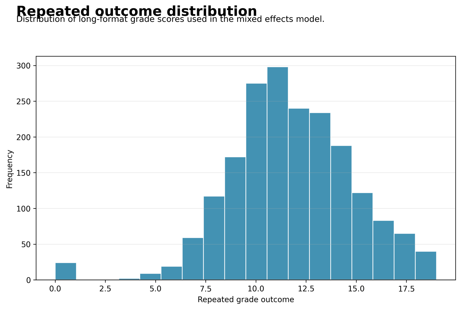
This histogram combines G1, G2 and G3 after the data are reshaped from one row per student to three rows per student. It shows the overall grade scale before the clustered model is fitted.
There are 1,947 repeated grade records. The period means are approximately 11.399 for G1, 11.570 for G2 and 11.906 for G3. Grade values range from 0 to 19.
The records are not 1,947 independent students. Every student contributes three related outcomes, so an ordinary regression would underestimate the similarity of observations from the same student.
Review Histogram Interpretation and Descriptive Statistics, then examine the ICC to quantify clustering.
Python Chart 2: Mean Grade by Period
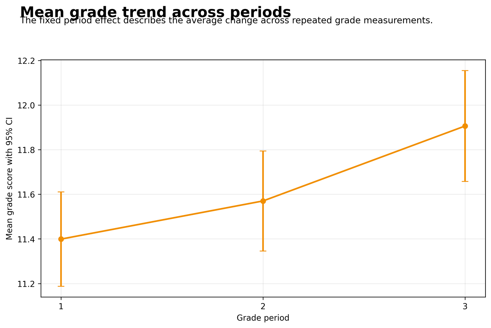
The chart summarizes the average repeated outcome at grade periods 1, 2 and 3. It provides an intuitive introduction to the fixed grade-period slope.
Mean grades are approximately 11.399, 11.570 and 11.906. The fitted grade_period coefficient is 0.2535, 95% CI [0.1941, 0.3128], p < .001.
After the other predictors are controlled, moving forward one grade period is associated with an average increase of about 0.253 grade points.
Distinguish a model-based fixed effect from a simple mean comparison. The Fixed Effects Regression guide explains average conditional effects.
Python Chart 3: Student Grade Profiles
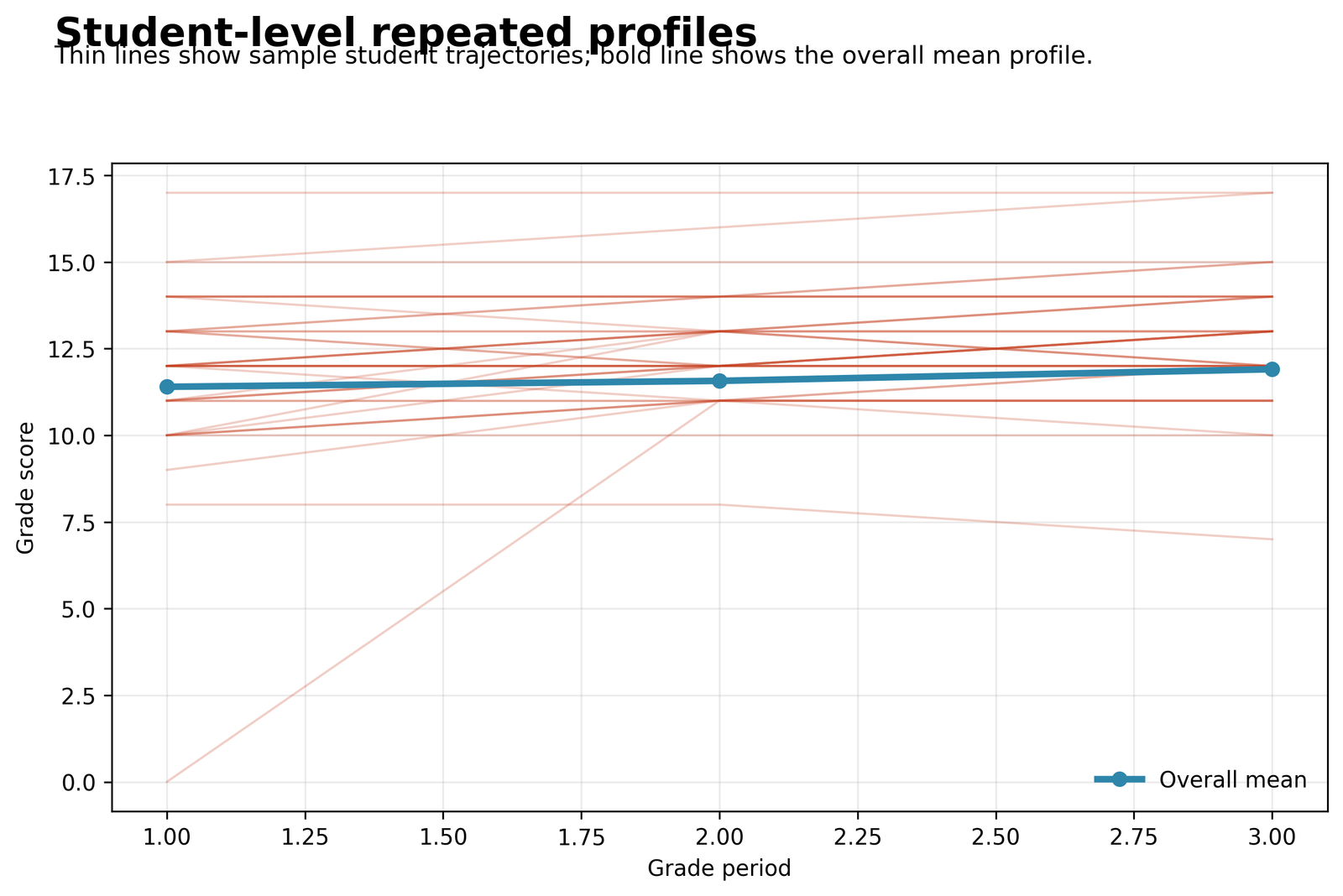
The profile plot shows why repeated observations from one student are related. Some students remain consistently high, some remain consistently low and others change across periods.
The dataset contains 649 student profiles, each with three grade measurements. The random-intercept variance is 5.3139, much larger than the within-student residual variance of 1.1909.
Students differ strongly in their underlying grade level. A student-specific random intercept moves the prediction line up or down while preserving the average fixed-effect slopes.
Read the Intraclass Correlation Coefficient guide to understand why repeated rows from the same student should be modeled together.
Python Chart 4: Observed vs Fitted Grade Scores
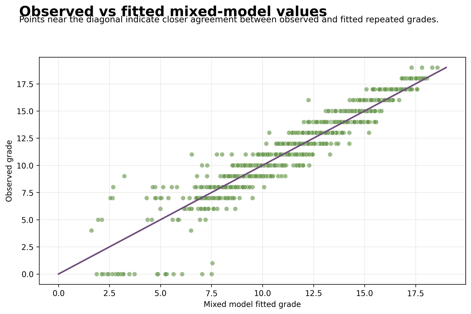
Points close to the agreement line indicate that the model reproduces the observed grade well. Conditional predictions benefit from knowing the student’s estimated random intercept.
The worked workbook reports a pseudo R² of 0.9073. The model uses 1,947 records and 649 random-intercept clusters.
The model explains much of the observed repeated-grade variation, partly because the student random intercept captures stable differences among students.
Do not treat a pseudo R² as identical to ordinary OLS R². Use Adjusted R-Squared for the ordinary-regression concept and report the mixed-model definition separately.
Python Chart 5: Residuals vs Fitted Values
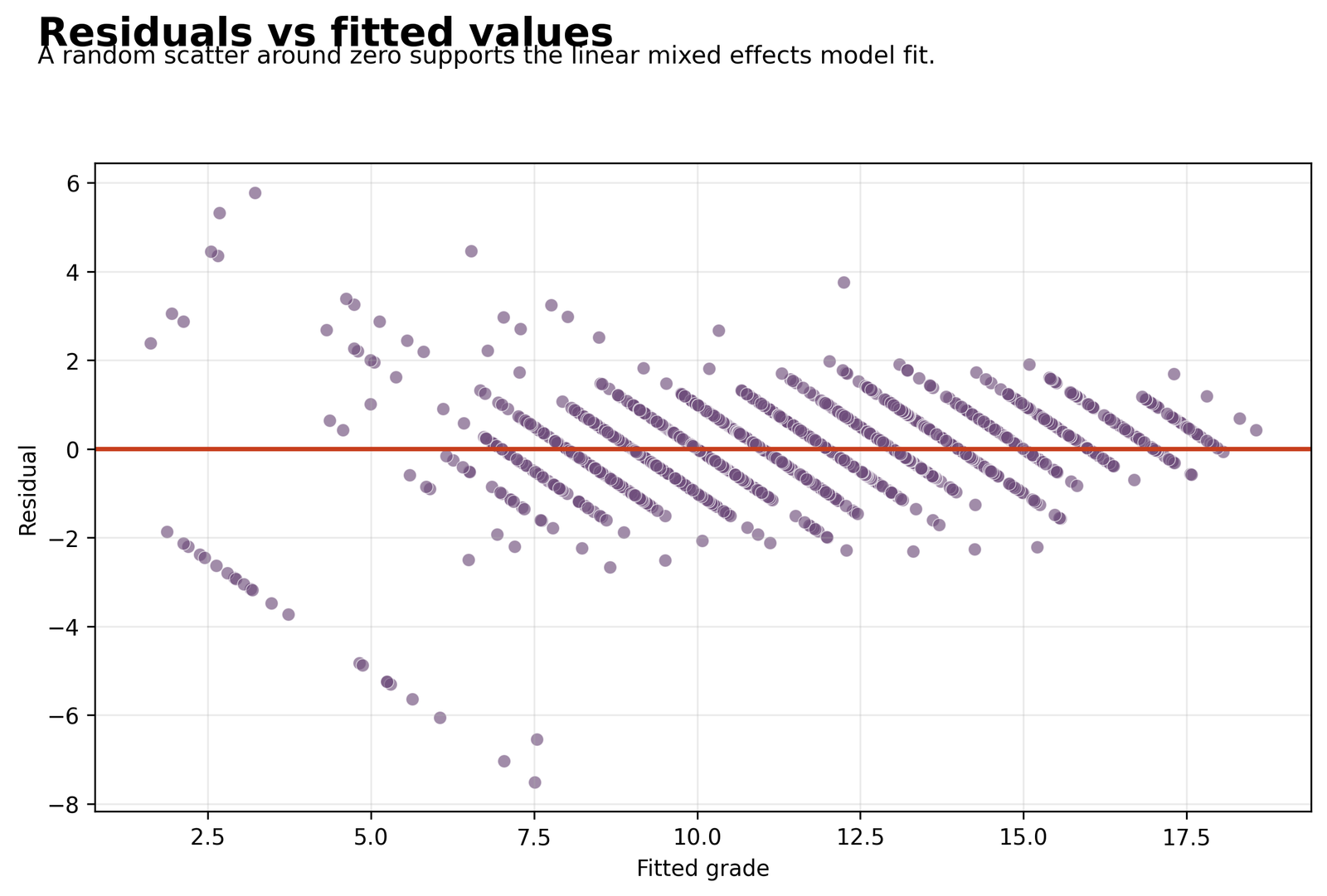
The residual plot checks whether errors stay centered near zero and whether their spread changes across fitted values.
The estimated residual variance is 1.1909, giving a residual standard deviation of approximately 1.0913. The workbook sample includes difficult cases such as a residual of -7.5062.
Most observations are predicted relatively closely, but some unexpectedly low grades create large negative residuals. These cases can affect normality and influence.
Use Studentized Residuals, Cook’s Distance and Influence Diagnostics.
Python Chart 6: Residual Distribution
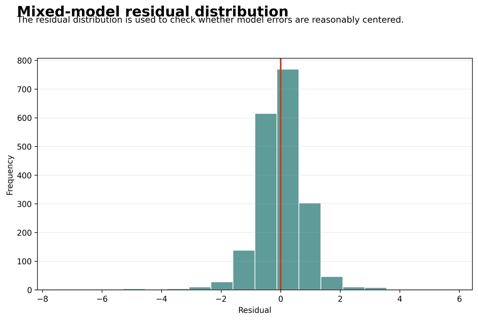
The figure shows whether most residuals are near zero and whether the distribution has long tails or strong asymmetry.
Within-student residual variance is 1.1909, representing 18.31% of the total residual variance. The corresponding standard deviation is approximately 1.0913.
A concentrated center supports good average fit, while extreme residuals indicate that not every grade follows the same predictable pattern.
Use a Q-Q Plot, P-P Plot and Shapiro-Wilk Test as supporting checks rather than judging normality from one histogram.
Python Chart 7: Student Random Intercepts
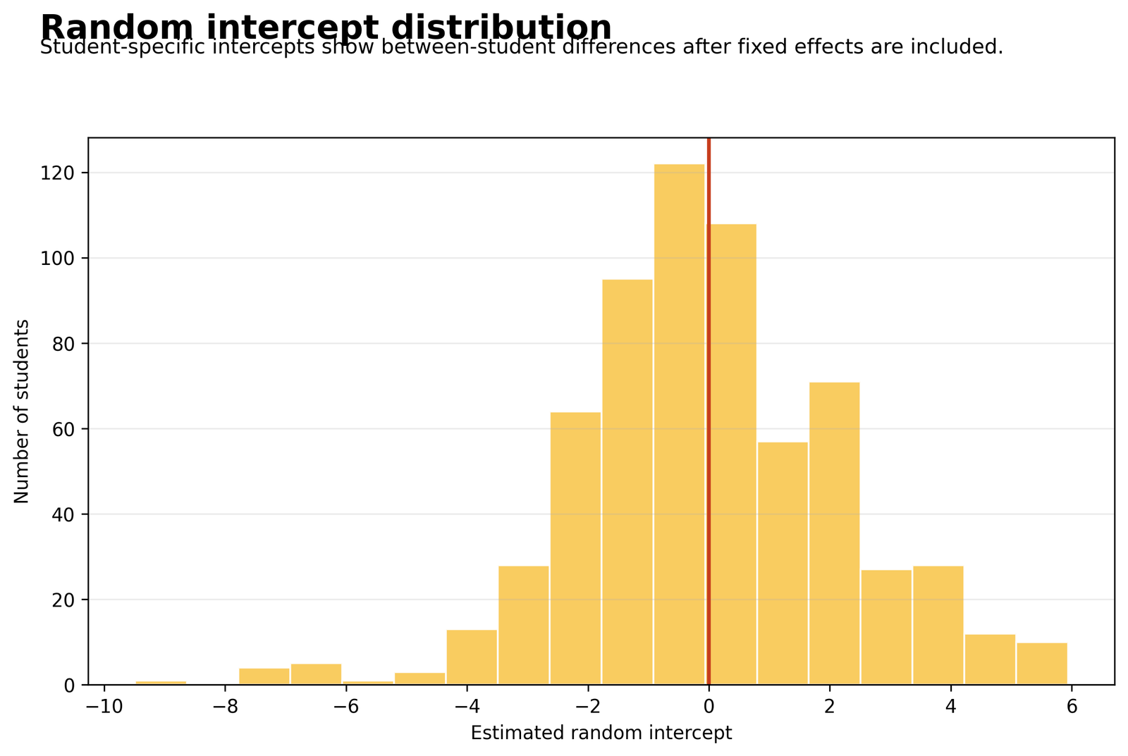
A positive random intercept raises all three fitted grades for a student; a negative value lowers them. The estimates are partially pooled toward zero.
Random-intercept variance is 5.3139, with standard deviation approximately 2.3052. The workbook sample includes values such as -5.7067 for student 1 and +3.9367 for student 16.
The large spread confirms that students differ substantially in their stable baseline performance, even after the fixed predictors are included.
Compare this idea with Random Effects ANOVA and Hierarchical Linear Modeling.
Python Chart 8: Fixed-Effect Coefficients
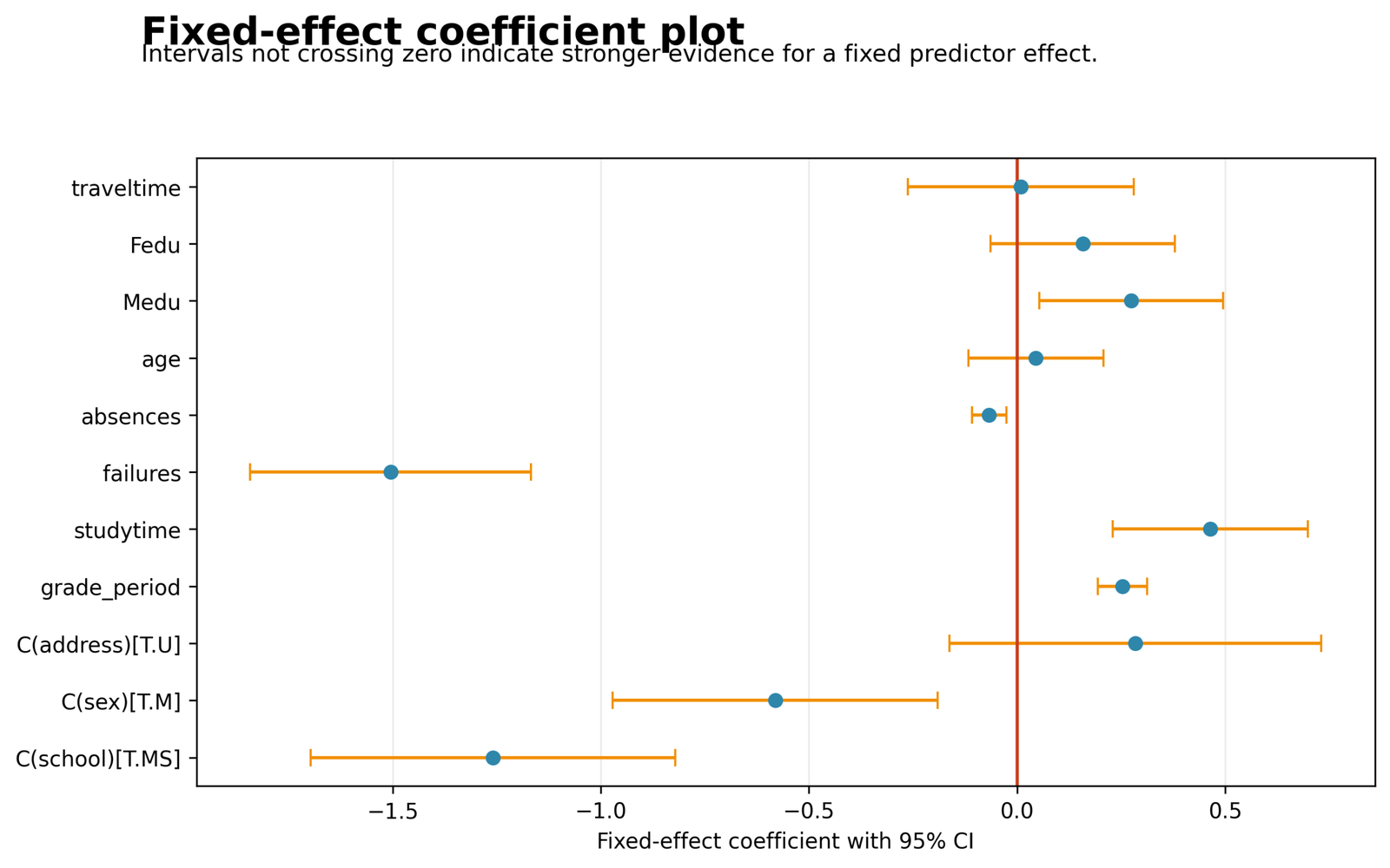
Each point is an estimated fixed coefficient and each horizontal interval shows uncertainty. Intervals crossing zero indicate that the adjusted effect is not statistically precise at the 5% level.
Strong significant terms include failures = -1.5051, school_MS = -1.2595, sex_M = -0.5811, studytime = 0.4639, Medu = 0.2741, grade_period = 0.2535 and absences = -0.0672.
Fixed effects describe average differences across all students. They do not replace random effects, which describe student-specific departures from the average intercept.
Use the Confidence Interval and P-Value guides to interpret precision without relying on significance labels alone.
Open the complete Python Mixed Effects Regression report PDF
R Mixed Effects Regression Visuals in Paired Layout
The R section groups two analytical visuals at a time. Two matching explanation boxes appear directly underneath. The only supplied R-specific hosted chart is the variance-components figure; the other panels are transparent HTML visualizations of the exact R/Excel model values.
Two-part model
Mean grade by period
R Visual 1: Mixed Effects Regression Model Structure
1,947 repeated rows are nested inside 649 students. Each student contributes G1, G2 and G3.
R Visual 2: Mean Grade by Period
G1 = 11.399, G2 = 11.570, G3 = 11.906; fixed period slope = 0.2535.
Variance shares
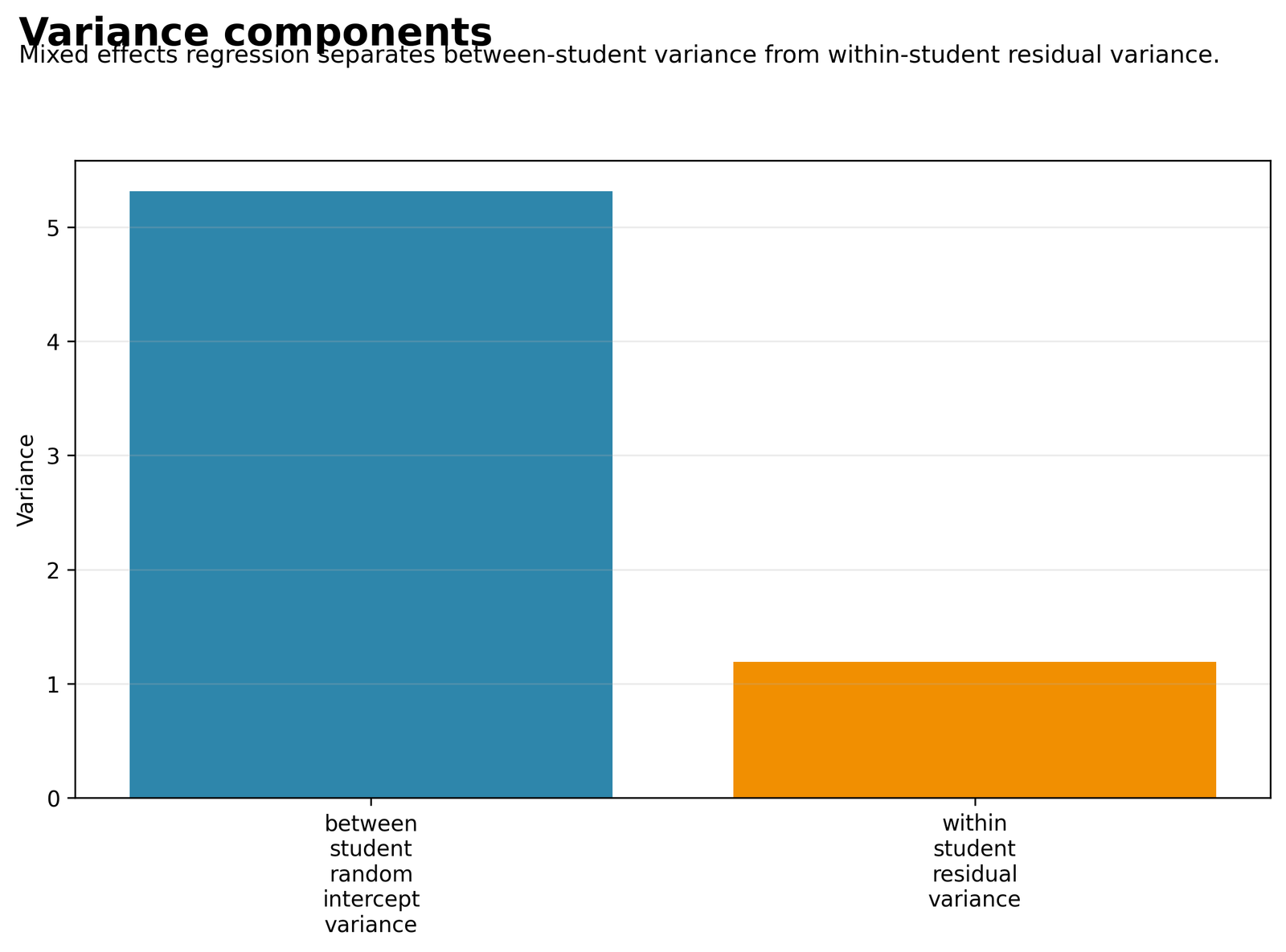
R Visual 3: Variance Components
Between-student variance = 5.3139; residual variance = 1.1909; total = 6.5048.
R Visual 4: ICC and Variance Shares
ICC = 0.8169; between-student share = 81.69%; within-student share = 18.31%.
Significant fixed effects
Intervals include zero
R Visual 5: Significant Fixed Effects
failures -1.5051; school_MS -1.2595; sex_M -0.5811; studytime +0.4639; Medu +0.2741; period +0.2535; absences -0.0672.
R Visual 6: Non-Significant Fixed Effects
address_U +0.2844; age +0.0452; Fedu +0.1579; traveltime +0.0086.
Fixed prediction contributions
Model summary
R Visual 7: Worked Prediction
The Excel calculator gives a fixed prediction of 12.5091 for period 3, studytime 2, failures 0, absences 4, age 17, Medu 2 and Fedu 2.
R Visual 8: Model Fit Summary
Pseudo R² = 0.9073; random-intercept SD = 2.3052; residual SD = 1.0913.
Mixed Effects Regression Fixed Effects
Fixed effects are the average coefficients shared by the population. They answer conditional questions after the repeated structure and all other predictors in the equation are considered.
| Term | Coefficient | SE | z | p | 95% CI | Decision |
|---|---|---|---|---|---|---|
| Intercept | 9.4579 | 1.4576 | 6.4886 | <.001 | [6.6010, 12.3147] | Significant |
| school_MS | -1.2595 | 0.2234 | -5.6384 | <.001 | [-1.6973, -0.8217] | Significant |
| sex_M | -0.5811 | 0.1992 | -2.9166 | .0035 | [-0.9716, -0.1906] | Significant |
| address_U | 0.2844 | 0.2279 | 1.2477 | .2121 | [-0.1623, 0.7310] | Not significant |
| grade_period | 0.2535 | 0.0303 | 8.3680 | <.001 | [0.1941, 0.3128] | Significant |
| studytime | 0.4639 | 0.1195 | 3.8814 | <.001 | [0.2297, 0.6982] | Significant |
| failures | -1.5051 | 0.1722 | -8.7377 | <.001 | [-1.8427, -1.1675] | Significant |
| absences | -0.0672 | 0.0211 | -3.1768 | .0015 | [-0.1086, -0.0257] | Significant |
| age | 0.0452 | 0.0826 | 0.5465 | .5848 | [-0.1168, 0.2071] | Not significant |
| Medu | 0.2741 | 0.1125 | 2.4374 | .0148 | [0.0537, 0.4945] | Significant |
| Fedu | 0.1579 | 0.1129 | 1.3991 | .1618 | [-0.0633, 0.3791] | Not significant |
| traveltime | 0.0086 | 0.1384 | 0.0619 | .9506 | [-0.2628, 0.2799] | Not significant |
Largest negative associations
Failures has the largest negative coefficient, -1.5051. MS school is -1.2595 relative to GP, and male students are -0.5811 relative to female students under the fitted coding.
Positive significant associations
Studytime is +0.4639, maternal education is +0.2741 and grade period is +0.2535. Their confidence intervals remain above zero.
A p-value answers whether the data are inconsistent with a zero coefficient under the model. A confidence interval is more informative because it shows both direction and precision. A coefficient can be statistically precise but still small in practical terms, so also review Effect Size.
Mixed Effects Regression Random Effects, ICC and Variance Components
Between-student variance
The random-intercept variance is 5.3139. Its square root is 2.3052, which is the standard deviation of the student intercept distribution. This tells us that student baselines vary substantially around the population intercept.
Within-student residual variance
The residual variance is 1.1909, with standard deviation 1.0913. This is the remaining variation among G1, G2 and G3 after the fixed predictors and student random intercept are considered.
Intraclass correlation coefficient
An ICC of 0.8169 means that approximately 81.69% of the model’s residual variation is associated with stable differences between students. Only 18.31% is within-student variation across grade records.
This very high ICC justifies the clustered model. Read the Intraclass Correlation Coefficient guide for formulas, interpretation and software comparisons.
Mixed Effects Regression Assumptions and Diagnostics
Beginner idea: model diagnostics ask whether the equation is a reasonable summary of the data and whether a small number of students or grade records control the results.
Fixed-part checks
- Relationships are reasonably linear.
- Categorical variables use correct references.
- Predictors are not destructively collinear.
- Important interactions or curves are not omitted.
Random-part checks
- Student clusters are correctly identified.
- Random intercepts are approximately well behaved.
- Within-student residuals are reasonably modeled.
- Independence is plausible between students.
Residual and influence checks
Use Studentized Residuals to find unusually large errors, Cook’s Distance and Influence Diagnostics to identify influential cases, and Mahalanobis Distance to find unusual predictor combinations.
Residual variance checks
The Breusch-Pagan Test and White Test are introductions to heteroskedasticity. Mixed-model residual structures may require more specialized variance modeling, but these guides explain the underlying idea.
Normality checks
Use a Q-Q Plot, P-P Plot, Shapiro-Wilk Test and Skewness and Kurtosis as complementary evidence. In large samples, formal tests can reject small departures that have limited practical impact.
Multicollinearity checks
Use the Multicollinearity Check, Variance Inflation Factor and Tolerance Statistic. Random effects do not automatically repair unstable fixed coefficients caused by strongly overlapping predictors.
Mixed Effects Regression in Python, R, SPSS and Excel
Python Mixed Effects Regression
Use statsmodels MixedLM after converting G1, G2 and G3 into long format. New Python users can begin with Correlation in Python for data and variable basics.
- Long-format reshaping
- Student random intercept
- Fixed coefficient table
- Residuals and random effects
R Mixed Effects Regression
Use lme4::lmer or nlme::lme with a random intercept for student_id. New R users can begin with Correlation in R.
- lmer fixed and random effects
- Variance components
- ICC calculation
- Conditional predictions
SPSS Mixed Effects Regression
Use Analyze → Mixed Models → Linear, identify student_id as the subject, specify grade_period as a repeated indicator if appropriate, and request fixed effects, covariance parameters and predictions. New SPSS users can begin with Correlation in SPSS.
- Subject = student_id
- Fixed predictors and factors
- Random intercept
- Covariance parameter output
Excel Mixed Effects Regression
Excel does not provide a standard built-in mixed-model optimizer, but the worked file explains the output, ICC and prediction equation. New users can begin with Correlation in Excel.
- Dashboard
- Fixed-effect lookup table
- Variance components
- Prediction calculator
Mixed Effects Regression Worked Excel File Explained
The workbook contains Dashboard, Fixed Effects, Variance Components, Prediction Calculator, Long Data Sample, Random Effects Sample and Excel Method sheets. It is a transparent companion to the Python and R analyses rather than a replacement for the mixed-model optimizer.
Dashboard
The Dashboard states that 649 students produce 1,947 long-format grade records. It reports ICC = 0.8169 and pseudo R² = 0.9073 and identifies student_id as the random-intercept cluster.
Fixed Effects sheet
This sheet contains every coefficient, standard error, z value, p value and 95% confidence interval. It also provides a lookup table used by the prediction calculator.
Variance Components sheet
The sheet calculates total variance as 5.3139 + 1.1909 = 6.5048 and ICC as 5.3139 ÷ 6.5048 = 0.8169.
Prediction Calculator
For period 3, studytime 2, failures 0, absences 4, age 17, Medu 2 and Fedu 2, the fixed prediction is 12.5091. A student’s random intercept can then be added to personalize the predicted grade.
Long Data Sample
The sample demonstrates how wide G1, G2 and G3 values become repeated rows with grade_score and grade_period. Formula columns calculate fixed predictions, residuals and squared residuals.
Mixed Effects Regression Code: Expand the Software You Need
Python statsmodels MixedLM code
import pandas as pd
import statsmodels.formula.api as smf

wide = pd.read_csv("dataset.csv").copy()
wide["student_id"] = range(1, len(wide) + 1)

long = wide.melt(
    id_vars=[
        "student_id", "studytime", "failures", "absences",
        "age", "Medu", "Fedu", "traveltime",
        "school", "sex", "address"
    ],
    value_vars=["G1", "G2", "G3"],
    var_name="grade_name",
    value_name="grade_score",
)

long["grade_period"] = long["grade_name"].map(
    {"G1": 1, "G2": 2, "G3": 3}
)

formula = (
    "grade_score ~ grade_period + studytime + failures"
    " + absences + age + Medu + Fedu + traveltime"
    " + C(school) + C(sex) + C(address)"
)

model = smf.mixedlm(
    formula,
    data=long,
    groups=long["student_id"],
    re_formula="1",
)

result = model.fit(reml=True, method="lbfgs")

print(result.summary())
print(result.cov_re)
print(result.scale)

long["fitted"] = result.fittedvalues
long["residual"] = long["grade_score"] - long["fitted"]
R lme4 code
library(tidyr)
library(dplyr)
library(lme4)

wide <- read.csv("dataset.csv")
wide$student_id <- seq_len(nrow(wide))

long <- wide |>
  pivot_longer(
    cols = c(G1, G2, G3),
    names_to = "grade_name",
    values_to = "grade_score"
  ) |>
  mutate(
    grade_period = recode(
      grade_name,
      G1 = 1L,
      G2 = 2L,
      G3 = 3L
    )
  )

model <- lmer(
  grade_score ~ grade_period + studytime + failures +
    absences + age + Medu + Fedu + traveltime +
    school + sex + address + (1 | student_id),
  data = long,
  REML = TRUE
)

summary(model)
VarCorr(model)
fixef(model)
ranef(model)

between_var <- as.numeric(VarCorr(model)$student_id)
within_var <- sigma(model)^2
icc <- between_var / (between_var + within_var)
SPSS MIXED syntax
* The data must be in long format with three rows per student.

MIXED grade_score BY school sex address
 WITH grade_period studytime failures absences age Medu Fedu traveltime
 /FIXED=INTERCEPT grade_period studytime failures absences
        age Medu Fedu traveltime school sex address | SSTYPE(3)
 /METHOD=REML
 /RANDOM=INTERCEPT | SUBJECT(student_id) COVTYPE(VC)
 /PRINT=SOLUTION TESTCOV
 /SAVE=FIXPRED PRED RESID.

OUTPUT SAVE
 /OUTFILE='D:\DATA ANALYSIS\H Regression Tests and Models\Mixed Effects Regression\SPSS_Output\spv\Mixed-Effects-Regression.spv'.

OUTPUT EXPORT
 /CONTENTS EXPORT=ALL LAYERS=PRINTSETTING MODELVIEWS=PRINTSETTING
 /PDF DOCUMENTFILE='D:\DATA ANALYSIS\H Regression Tests and Models\Mixed Effects Regression\SPSS_Output\pdf\Mixed-Effects-Regression-SPSS-Output.pdf'.
Excel formulas
Total variance:
=Between_Student_Variance+Residual_Variance

ICC:
=Between_Student_Variance/Total_Variance

Random-intercept SD:
=SQRT(Between_Student_Variance)

Residual SD:
=SQRT(Residual_Variance)

Fixed prediction:
=Intercept
 + Grade_Period*Beta_Period
 + Studytime*Beta_Studytime
 + Failures*Beta_Failures
 + Absences*Beta_Absences
 + Age*Beta_Age
 + Medu*Beta_Medu
 + Fedu*Beta_Fedu
 + Traveltime*Beta_Traveltime
 + Dummy_Variable_Contributions

Conditional prediction:
=Fixed_Prediction+Student_Random_Intercept

Residual:
=Observed_Grade-Conditional_Prediction
How a New Student Should Study This Mixed Effects Regression Example
- Identify the cluster: student_id is the grouping variable.
- Identify the repeated outcome: G1, G2 and G3 become grade_score.
- Separate fixed and random effects: fixed effects are average slopes; the random intercept is student-specific.
- Read the variance components: 5.3139 is between students and 1.1909 is within students.
- Calculate the ICC: 5.3139 divided by 6.5048 equals 0.8169.
- Interpret fixed coefficients: state the direction, unit and reference category.
- Read diagnostics: check residuals, random effects and influential cases.
- Write the conclusion: report both the average effects and the strong student clustering.
Before moving to advanced material, make sure you can explain the method without formulas: the model predicts repeated grades, estimates average relationships and adjusts every student’s prediction with a personal baseline.
For foundations, review Descriptive Statistics, Variance, Standard Deviation and Confidence Interval.
Advanced Mixed Effects Regression Interpretation and Extensions
The main reading path remains beginner-friendly. Expand only the technical topics needed for the research question.
Why the long format matters
- Wide data place G1, G2 and G3 in separate columns.
- Long data place the repeated value in grade_score and identify the occasion with grade_period.
- Most mixed-model software expects one row per observation.
How to read the intercept
- The intercept is 9.4579 under zero values and reference categories.
- Some zero values are not substantively typical, so centering can improve interpretation.
- Changing centering changes the intercept but not fitted values.
How to read grade_period
- The model treats periods 1, 2 and 3 as equally spaced.
- The 0.2535 coefficient is one linear average increase per period.
- Treat period as categorical if equal spacing or linearity is doubtful.
How to understand school_MS
- The coefficient compares MS with GP.
- The estimate is conditional on all other fixed predictors.
- It should not be interpreted as a causal school effect.
How to understand sex_M
- The coefficient compares male with female students.
- Reference coding affects the displayed sign.
- The fitted values and overall information do not depend on which category is named first.
Why address_U is not significant
- The estimate is positive but imprecise.
- Its interval extends below and above zero.
- Report the estimate and interval rather than writing that there is no effect.
How random effects improve predictions
- Fixed predictions describe a student with random intercept zero.
- Conditional predictions add the estimated student intercept.
- Prediction for a new student requires integrating over or setting the unknown random effect.
Predictions for new clusters
- A new student has no estimated random intercept.
- Use the population-average fixed prediction initially.
- Update the student-specific prediction after repeated observations become available.
Shrinkage of random effects
- Extreme random-intercept estimates are pulled toward zero.
- The amount of shrinkage depends on information and variance.
- Shrinkage improves stability compared with separate intercepts for every student.
Why three periods limit random slopes
- Only three outcomes are available per student.
- A random slope can be fitted but may be less stable.
- Model complexity should follow data support and theory.
Checking convergence
- Optimization must reach a stable solution.
- Warnings can indicate over-complex random effects or poor scaling.
- Try justified simplification rather than ignoring warnings.
Singular fits
- A singular fit means one or more random-effect dimensions are estimated near zero or perfectly correlated.
- It often signals an overly complex random structure.
- The current random-intercept-only model is comparatively simple.
Cluster-level confounding
- School-level or student-level omitted variables can affect fixed estimates.
- A random intercept represents unexplained baseline heterogeneity but does not remove all confounding.
- Causal claims require stronger design assumptions.
Within-between decomposition
- A time-varying predictor can be split into a student mean and a deviation from that mean.
- The two coefficients answer different questions.
- This decomposition prevents a within-person effect from being confused with a between-person effect.
Handling irregular time
- grade_period assumes equally spaced occasions.
- Actual dates can replace period numbers when intervals differ.
- Nonlinear time functions may be needed for irregular growth.
Modeling ceiling and floor effects
- Grades are bounded between 0 and 19.
- A Gaussian model can predict outside the theoretical range in extreme profiles.
- Sensitivity analysis may consider ordinal or bounded-outcome approaches.
Residual versus random-effect outliers
- A residual outlier is unusual for one occasion.
- A random-effect outlier is a cluster with an unusual baseline.
- The two types require different investigation.
Why large samples can produce small p-values
- There are 1,947 grade rows and 649 clusters.
- Small coefficients may become statistically precise.
- Interpret practical magnitude and confidence intervals.
Planning future studies
- Power depends on clusters, observations per cluster, ICC and effect size.
- Adding clusters is often more valuable than adding many observations to the same few clusters.
- Simulation is useful for complex mixed models.
Communicating mixed models
- Begin with the data structure before presenting formulas.
- Explain the fixed and random parts separately.
- Use the ICC to connect the design with the model choice.
Mixed Effects Regression versus ordinary regression
- Ordinary regression assumes independent rows.
- The mixed model represents dependence through a random-effect distribution.
- Coefficient interpretation remains conditional on all included predictors.
Mixed Effects Regression versus repeated-measures ANOVA
- Repeated-measures ANOVA is useful for balanced repeated factors.
- Mixed Effects Regression handles unequal observations, continuous predictors and flexible covariance structures more naturally.
- Read Repeated Measures ANOVA for the classical comparison.
Mixed Effects Regression versus GEE
- The mixed model gives cluster-specific effects and random effects.
- GEE gives population-average effects with robust sandwich uncertainty.
- The scientific target should determine the method.
Random intercept versus random slope
- A random intercept allows students to begin at different levels.
- A random slope allows the grade-period trend to differ among students.
- Random slopes require enough repeated information and stable estimation.
Why the ICC is high
- Stable academic differences persist across G1, G2 and G3.
- The between-student variance is more than four times the residual variance.
- High clustering makes independence-based analysis especially inappropriate.
Partial pooling
- Random-intercept estimates are pulled toward the population average.
- Students with less information receive stronger shrinkage.
- Partial pooling reduces unstable extreme estimates.
Conditional versus marginal predictions
- Conditional predictions include the student random intercept.
- Marginal predictions use only the fixed effects.
- State which prediction type is plotted or reported.
REML versus maximum likelihood
- REML is commonly preferred for variance-component estimation.
- Maximum likelihood is used when comparing models with different fixed effects.
- Compare models only under compatible estimation settings.
Testing random effects
- Variance parameters lie on a boundary at zero.
- Ordinary chi-square approximations can be inaccurate.
- Likelihood-ratio tests, restricted tests or bootstrap methods may be used.
Random-effect normality
- The standard random-intercept model assumes an approximately normal distribution.
- Estimated random effects are shrunken predictions, not raw observations.
- Use plots and sensitivity checks rather than one formal test alone.
Residual covariance structures
- A random intercept creates compound-symmetry-like correlation.
- Repeated observations may also show time-dependent residual correlation.
- SPSS and nlme can compare alternative covariance structures.
Unequal observation counts
- Mixed models can retain students with different numbers of measurements under suitable missing-data assumptions.
- This example is balanced with three grades per student.
- Unbalanced longitudinal data are a major practical advantage of the method.
Missing data assumptions
- Likelihood-based mixed models are often valid under missing at random conditional on the model.
- Missing not at random mechanisms require sensitivity analysis.
- Describe missingness by period and student characteristics.
Centering predictors
- Grand-mean centering changes the intercept to an average-profile interpretation.
- Group-mean centering separates within-cluster and between-cluster effects for time-varying predictors.
- The correct centering depends on the scientific question.
Time-varying and time-invariant predictors
- grade_period varies within student.
- School, sex and parental education are treated as student-level variables.
- A time-varying predictor can have separate within- and between-student components.
Cross-level interactions
- A student-level variable can modify a within-student period slope.
- Interactions require careful coding and sufficient clusters.
- Interpret conditional effects at meaningful moderator values.
Nonlinear time trends
- Three periods can support a simple linear trend but may also show curvature.
- Add a quadratic term only when theory and data justify it.
- Treating period as categorical avoids imposing a linear shape.
Model comparison
- Use likelihood-ratio tests, AIC and BIC under compatible estimation.
- Do not compare REML likelihoods across different fixed-effect structures.
- Prediction and scientific interpretability also matter.
Pseudo R-squared
- Several mixed-model R² definitions exist.
- Marginal R² reflects fixed effects; conditional R² includes random effects.
- Always name the formula or software definition used.
Cluster count and power
- Power depends strongly on the number of independent clusters.
- A large number of rows cannot compensate fully for very few clusters.
- Use Statistical Power when planning a new study.
Fixed-effect confidence intervals
- Intervals show plausible coefficient values under the model.
- A narrow interval indicates greater precision.
- Practical importance should be considered alongside exclusion of zero.
Interpreting categorical effects
- school_MS compares MS with GP.
- sex_M compares male with female.
- address_U compares urban with rural.
Why age is non-significant
- The adjusted age coefficient is 0.0452 with an interval that crosses zero.
- This does not prove age is unrelated to grade in every population.
- It means the model does not estimate a precise conditional age effect here.
Why failures is strongly negative
- Each additional previous failure is associated with about 1.505 lower grade points.
- The interval remains fully below zero.
- The result is conditional and not automatically causal.
Why school has a negative contrast
- MS is estimated 1.2595 points below GP under the chosen coding.
- Unmeasured school-level factors may contribute.
- With only two schools, broad population generalization requires caution.
Influence at two levels
- One unusual grade record can affect the residual structure.
- One unusual student profile can affect fixed and random estimates.
- Diagnostics should inspect observations and clusters.
Bootstrap and robust inference
- Cluster bootstrap resamples students rather than individual grade rows.
- Robust standard errors can address some covariance misspecification.
- Neither approach repairs an incorrect mean structure.
Binary and count mixed models
- A binary outcome requires mixed-effects logistic regression.
- A count outcome may require Poisson or negative-binomial mixed modeling.
- Choose the outcome family before interpreting coefficients.
Nested and crossed random effects
- Students nested in schools create a multilevel hierarchy.
- Crossed effects arise when observations belong to multiple non-nested groups.
- The current model uses one student random intercept only.
Reproducibility
- Save the wide-to-long transformation, formula and reference categories.
- Record estimation method, software version and convergence messages.
- Export fixed effects, random effects, variance components and predictions.
APA-Style Reporting for Mixed Effects Regression
Mixed Effects Regression Publication Checklist and Common Mistakes
Report these items
- Outcome and repeated-measure structure
- Cluster variable and number of clusters
- Fixed predictors and reference categories
- Random-effects structure
- Estimation method
- Fixed coefficients, SEs and confidence intervals
- Variance components and ICC
- Residual and random-effect diagnostics
- Marginal or conditional prediction type
- Software and convergence information
Avoid these mistakes
- Treating repeated rows as independent
- Confusing a random intercept with a residual
- Calling the ICC an ordinary R²
- Interpreting random effects as fixed coefficients
- Ignoring reference categories
- Comparing incompatible REML likelihoods
- Adding complex random slopes without support
- Reporting only p-values
- Deleting extreme students automatically
- Ignoring convergence warnings
Mixed Effects Regression Downloads
R Mixed Effects Regression ReportCross-software model validation, variance components and outputs.
Mixed Effects Regression Worked Excel FileDashboard, coefficients, ICC, prediction calculator and sample rows.
Hierarchical Linear Model GuideContinue to broader multilevel structures and random effects.
Frequently Asked Questions About Mixed Effects Regression
What is Mixed Effects Regression?
Mixed Effects Regression combines population-average fixed effects with group-specific random effects.
Why is it called mixed?
It contains both fixed and random effects in one equation.
What is the cluster in this example?
student_id is the cluster because each student contributes G1, G2 and G3.
How many observations are analyzed?
There are 1,947 repeated grade records.
How many students are analyzed?
There are 649 student clusters.
What is the outcome?
grade_score is the long-format outcome created from G1, G2 and G3.
What is a random intercept?
It is a student-specific adjustment that raises or lowers all fitted grades for that student.
What are fixed effects?
They are average coefficients shared across students.
What is the ICC?
The ICC is 0.8169.
How is the ICC calculated?
Divide 5.3139 by the total variance 6.5048.
What does an ICC of 0.8169 mean?
About 81.69% of residual variation is between students.
What is the within-student share?
The residual share is approximately 18.31%.
What is the period effect?
Each one-period increase is associated with about 0.2535 higher grade points after adjustment.
What is the strongest negative coefficient?
Failures has B = -1.5051.
What does the studytime coefficient mean?
One category increase in studytime is associated with about 0.4639 higher grade points.
What does the absences coefficient mean?
Each additional absence is associated with about 0.0672 lower grade points.
Is age significant?
No. Its confidence interval includes zero and p = .5848.
Is maternal education significant?
Yes. Medu has B = 0.2741 and p = .0148.
Is paternal education significant?
No. Fedu has p = .1618.
What is pseudo R-squared?
It is a mixed-model fit summary whose definition should be reported explicitly.
Can ordinary regression be used instead?
It would ignore the strong dependence among three grades from the same student.
Can repeated-measures ANOVA be used?
It can answer simpler balanced questions, but the mixed model handles predictors and random effects more flexibly.
What is the difference between a random intercept and random slope?
A random intercept changes the baseline; a random slope changes a predictor effect across clusters.
Can SPSS run the model?
Yes. Use Linear Mixed Models with student_id as the subject and a random intercept.
Can R run the model?
Yes. lme4::lmer and nlme::lme are common options.
Can Python run the model?
Yes. statsmodels MixedLM can fit the random-intercept model.
Can Excel estimate the complete model?
Excel is best used here for understanding, calculations and reporting rather than optimization.
What diagnostics are important?
Check residuals, random-effect shape, influence, multicollinearity and convergence.
Does a high ICC prove causation?
No. It describes clustering, not causal relationships.
How should the result be summarized?
Report the fixed effects, random-intercept variance, residual variance, ICC, cluster count and diagnostics.
Final Mixed Effects Regression Conclusion
Mixed Effects Regression should always be explained by identifying the repeated unit, the cluster, the fixed part and the random part.
Mixed Effects Regression predictions must be labeled as fixed-only or conditional on a random effect.
Mixed Effects Regression reporting should connect every variance component with the actual data hierarchy.
Mixed Effects Regression is most useful when observations within the same group are more similar than observations from different groups.
Mixed Effects Regression should always be explained by identifying the repeated unit, the cluster, the fixed part and the random part.
Mixed Effects Regression predictions must be labeled as fixed-only or conditional on a random effect.
Mixed Effects Regression reporting should connect every variance component with the actual data hierarchy.
Mixed Effects Regression is most useful when observations within the same group are more similar than observations from different groups.
Mixed Effects Regression should always be explained by identifying the repeated unit, the cluster, the fixed part and the random part.
Mixed Effects Regression predictions must be labeled as fixed-only or conditional on a random effect.
Mixed Effects Regression reporting should connect every variance component with the actual data hierarchy.
Mixed Effects Regression is most useful when observations within the same group are more similar than observations from different groups.
Mixed Effects Regression should always be explained by identifying the repeated unit, the cluster, the fixed part and the random part.
Mixed Effects Regression predictions must be labeled as fixed-only or conditional on a random effect.
Mixed Effects Regression reporting should connect every variance component with the actual data hierarchy.
Mixed Effects Regression is most useful when observations within the same group are more similar than observations from different groups.
Mixed Effects Regression should always be explained by identifying the repeated unit, the cluster, the fixed part and the random part.
Beginner conclusion: the three grades from one student are related, so they should not be analyzed as independent rows. Mixed Effects Regression represents that dependence with a student random intercept.
The analysis contains 1,947 repeated grades from 649 students. Between-student variance is 5.3139 and within-student residual variance is 1.1909, producing ICC = 0.8169. This means student membership explains most of the clustering in the repeated outcomes.
After that clustering is modeled, later grade periods, studytime and maternal education are positively associated with grade score, while failures, absences, MS school and male sex have negative adjusted coefficients under the specified coding.

