
Pooled OLS, One-Way and Multi-Way Group Controls, Within Transformation and Model Comparison
Fixed Effects Regression: Interpretation, SPSS, Python, R and Excel Guide
Fixed Effects Regression controls for systematic differences across named groups by including group indicators or by removing group means before estimation. This worked example predicts G3 final grade from eight numeric predictors and fixed effects for school, sex, address and higher-education intention. It compares pooled OLS, one-way school fixed effects and multi-way fixed effects, then explains adjusted R squared, nested F tests, coefficients, within-transformed relationships, Python and R charts, SPSS output and Excel formulas.
Quick Answer: Fixed Effects Regression Result
The verified workbook contains 649 complete observations. The outcome is G3. Numeric predictors are G1, G2, studytime, failures, absences, age, Medu and Fedu. The multi-way fixed-effects specification adds indicator variables for school, sex, address and higher, with GP, F, R and no used as the reference levels implied by the coefficient labels.
The multi-way model has R² = 0.852652, adjusted R² = 0.849872, RMSE = 1.239162 and MAE = 0.777422. It has the highest adjusted R² among the three displayed models. However, its nested improvement over pooled OLS is not statistically significant at alpha .05, F = 2.022938, df difference = 4, p = 0.089644.
Main interpretation: G2 is the dominant adjusted predictor of G3, B = 0.8792, 95% CI [0.8117, 0.9466], p < .001. G1 is also positive, B = 0.1313, p = .0004, while failures is negative, B = -0.2178, p = .0233. The four fixed-effect dummy coefficients all have p-values above .05 after the numeric predictors are controlled.
Model-selection conclusion: the multi-way model is best only under the adjusted-R² criterion. One-way fixed effects has the lowest AIC, 2145.5751, while pooled OLS has the lowest BIC, 2186.6036. The nested F tests do not show a significant fixed-effect improvement at .05. The correct conclusion is therefore criterion-specific rather than “multi-way fixed effects is unquestionably superior.”
Terminology note: this workbook demonstrates a least-squares dummy-variable fixed-effects model on one cross-sectional student dataset. Classical panel fixed-effects regression usually controls for repeated entity-specific intercepts across time. The algebra is related, but the data structure and causal interpretation are not automatically the same.
Table of Contents
- What Is Fixed Effects Regression?
- One-Way, Two-Way and Multi-Way Fixed Effects
- Fixed Effects Equations and Within Transformation
- When to Use Fixed Effects Regression
- Dataset and Variables Used
- Pooled OLS vs Fixed Effects Model Comparison
- Coefficient Interpretation
- Fixed-Effect Group Means and Coefficients
- Nested F Tests and Decision Rules
- Fixed Effects Regression Assumptions
- Within, Between and Total Variation
- Fixed Effects vs Random Effects
- Python Chart-by-Chart Interpretation
- R Charts, Tables and Independent Validation
- SPSS Output Interpretation
- Excel Worked Results and Formulas
- Python, R, SPSS and Excel Workflows
- Fixed Effects Regression Code
- Robust and Clustered Standard Errors
- APA-Style Reporting
- Reporting Checklist
- Common Mistakes
- Troubleshooting Guide
- Downloads and Resources
- Related Salar Cafe Guides
- FAQs
What Is Fixed Effects Regression?
Fixed Effects Regression controls for group-specific intercept differences that might otherwise be absorbed into the error term and confound the coefficients of interest. In a least-squares dummy-variable model, each nonreference group receives an indicator coefficient. In a within-transformed panel model, group means are subtracted from the outcome and time-varying predictors so that estimation uses variation within the same entity.
The term “fixed effect” can be used in several ways. In experimental ANOVA, a fixed factor has levels chosen because those exact levels are substantively important. In regression, fixed effects often mean a complete set of group indicators. In panel econometrics, entity fixed effects control all time-invariant characteristics of each entity, whether those characteristics were measured or not.
Simple definition: fixed effects allow each included group to have its own intercept while estimating common slopes for the numeric predictors, unless interactions or varying slopes are added.
What Fixed Effects Control
A group dummy controls for average level differences between that group and the reference group. In repeated panel data, an entity fixed effect controls all characteristics that remain constant within the entity across time. This can reduce omitted-variable bias from stable unmeasured differences.
What Fixed Effects Do Not Automatically Control
Fixed effects do not remove bias from time-varying omitted variables, measurement error, reverse causation, incorrect functional form or selection mechanisms. Adding many group dummies does not transform an observational association into a causal effect without a defensible research design.
One-Way, Two-Way and Multi-Way Fixed Effects
| Specification | Fixed Effects Included | Example | Interpretation |
|---|---|---|---|
| Pooled OLS | None | G3 predicted only from eight numeric predictors. | All observations share one intercept. |
| One-way fixed effects | One grouping dimension | Add school indicators. | GP and MS may have different intercepts. |
| Two-way fixed effects | Two grouping dimensions | Entity and year in panel data. | Controls stable entity differences and common time shocks. |
| Multi-way fixed effects | Several grouping dimensions | Add school, sex, address and higher indicators. | Each included grouping dimension contributes intercept adjustments. |
| Fixed effects with interactions | Group effects plus effect modification | G2 × school. | Allows a numeric slope to differ across groups. |
The workbook compares pooled OLS with a one-way school fixed-effects model and a multi-way model containing four grouping dimensions. The one-way model has nine slope degrees of freedom: eight numeric predictors plus one school dummy. The multi-way model has twelve slope degrees of freedom: eight numeric predictors plus four group dummies.
Fixed Effects Regression Equations and Within Transformation
Least-Squares Dummy-Variable Equation
The intercept represents the expected G3 for the reference categories when numeric predictors equal zero. Each numeric coefficient is interpreted while holding the other numeric predictors and fixed-effect dummies constant. Each dummy coefficient represents an adjusted intercept difference from its reference group.
Panel Fixed-Effects Equation
Here, αᵢ is an entity fixed effect and λₜ may be a time fixed effect. Repeated observations are required to estimate within-entity change. Time-invariant predictors cannot be separately identified from entity fixed effects because they disappear under demeaning.
Within Transformation
Subtracting each entity’s mean removes the entity-specific intercept. In the uploaded workbook’s chart demonstration, G2 and G3 are demeaned within the combined school × sex × address × higher cells. The within-transformed G2–G3 correlation is 0.902094, and the simple within slope is approximately 0.987075.
Important distinction: the combined-group demeaning chart is educational. It is not identical to a repeated-entity panel estimator because each student appears once. The full regression result comes from dummy-variable OLS with the named group controls.
When to Use Fixed Effects Regression
| Research Situation | Use Fixed Effects? | Reason |
|---|---|---|
| Repeated observations for the same schools, firms, countries or people | Often yes | Entity fixed effects control stable unobserved group differences. |
| Common shocks vary by year | Add time fixed effects | Year indicators absorb shocks shared by all entities. |
| Cross-sectional data with known group categories | Possible | Dummy-variable controls adjust intercept differences across observed groups. |
| Interest is in a time-invariant predictor under entity FE | Not identified directly | The predictor is collinear with the entity fixed effects. |
| Group effects are uncorrelated with predictors and population inference is desired | Consider random effects | Random effects may be more efficient under stronger assumptions. |
| Only one observation per entity and thousands of individual dummies | Usually not meaningful | There is no within-entity variation to estimate a panel fixed effect. |
Fixed effects are particularly useful when omitted stable group characteristics are likely to correlate with the predictors. They are less useful when the main predictors have almost no within-group variation or when the group indicators consume too much information relative to sample size.
Dataset and Variables Used
The worked analysis uses 649 complete student records. The outcome is G3. Eight numeric predictors enter all three models. The one-way model adds school, while the multi-way model adds school, sex, address and higher-education intention.
Outcome and Numeric Predictor Dictionary
| Variable | Role | Plain-English Meaning | Coefficient Unit |
|---|---|---|---|
| G3 | Outcome | Final grade, observed from 0 to 19. | Predicted final-grade points. |
| G1 | Numeric predictor | First-period grade. | G3 change for a one-point G1 increase. |
| G2 | Numeric predictor | Second-period grade. | G3 change for a one-point G2 increase. |
| studytime | Numeric predictor | Weekly study-time category. | G3 change for one category higher studytime. |
| failures | Numeric predictor | Number of previous class failures. | G3 change for one additional failure. |
| absences | Numeric predictor | School absence count. | G3 change for one additional absence. |
| age | Numeric predictor | Student age. | G3 change for one additional year. |
| Medu | Numeric predictor | Mother’s education level. | G3 change for one level higher Medu. |
| Fedu | Numeric predictor | Father’s education level. | G3 change for one level higher Fedu. |
Fixed-Effect Group Dictionary and Reference Categories
| Fixed-Effect Variable | Dummy Term | Reference Category | Compared Category | Interpretation |
|---|---|---|---|---|
| school | C(school)[T.MS] | GP | MS | Adjusted intercept difference between MS and GP. |
| sex | C(sex)[T.M] | F | M | Adjusted intercept difference between M and F. |
| address | C(address)[T.U] | R | U | Adjusted intercept difference between urban and rural address. |
| higher | C(higher)[T.yes] | no | yes | Adjusted intercept difference for intending higher education. |
Complete Model Specifications
| Model | Numeric Terms | Fixed Effects | Slope df |
|---|---|---|---|
| Pooled OLS | G1, G2, studytime, failures, absences, age, Medu, Fedu | None | 8 |
| One-way fixed effects | Same eight numeric predictors | school | 9 |
| Multi-way fixed effects | Same eight numeric predictors | school, sex, address, higher | 12 |
Pooled OLS vs One-Way and Multi-Way Fixed Effects
| Model | N | df Model | R² | Adjusted R² | RMSE | MAE | F Statistic | AIC | BIC |
|---|---|---|---|---|---|---|---|---|---|
| Pooled OLS | 649 | 8 | 0.850777 | 0.848912 | 1.247020 | 0.780019 | 456.1111 | 2146.3247 | 2186.6036 |
| One-way fixed effects | 649 | 9 | 0.851408 | 0.849315 | 1.244381 | 0.778888 | 406.8187 | 2145.5751 | 2190.3294 |
| Multi-way fixed effects | 649 | 12 | 0.852652 | 0.849872 | 1.239162 | 0.777422 | 306.6924 | 2146.1196 | 2204.3002 |
The multi-way model increases R² by 0.001875 over pooled OLS and increases adjusted R² by 0.000960. RMSE decreases by approximately 0.007858, while MAE decreases by about 0.002596. These are real improvements but small in practical magnitude.
One-way fixed effects has the lowest AIC, beating pooled OLS by about 0.750 and multi-way fixed effects by about 0.545. Pooled OLS has the lowest BIC because BIC penalizes the additional fixed-effect parameters more strongly. A responsible report names the criterion used rather than selecting whichever statistic supports the preferred model.
Fixed Effects Regression Coefficient Interpretation
| Term | Coefficient | SE | t Value | p-value | 95% Confidence Interval | Decision |
|---|---|---|---|---|---|---|
| Intercept | -0.4214 | 0.8185 | -0.5149 | 0.6068 | -2.0288 to 1.1859 | Not significant |
| school: MS vs GP | -0.1759 | 0.1192 | -1.4758 | 0.1405 | -0.4100 to 0.0582 | Not significant |
| sex: M vs F | -0.1887 | 0.1046 | -1.8041 | 0.0717 | -0.3942 to 0.0167 | Not significant |
| address: U vs R | 0.1077 | 0.1152 | 0.9352 | 0.3500 | -0.1185 to 0.3339 | Not significant |
| higher: yes vs no | 0.1870 | 0.1795 | 1.0420 | 0.2978 | -0.1654 to 0.5394 | Not significant |
| G1 | 0.1313 | 0.0369 | 3.5576 | 0.0004 | 0.0588 to 0.2037 | Significant positive |
| G2 | 0.8792 | 0.0343 | 25.6035 | < .001 | 0.8117 to 0.9466 | Significant positive |
| studytime | 0.0584 | 0.0637 | 0.9176 | 0.3592 | -0.0666 to 0.1834 | Not significant |
| failures | -0.2178 | 0.0958 | -2.2734 | 0.0233 | -0.4060 to -0.0297 | Significant negative |
| absences | 0.0182 | 0.0112 | 1.6208 | 0.1055 | -0.0038 to 0.0402 | Not significant |
| age | 0.0311 | 0.0444 | 0.7000 | 0.4842 | -0.0561 to 0.1182 | Not significant |
| Medu | -0.0536 | 0.0588 | -0.9106 | 0.3629 | -0.1691 to 0.0620 | Not significant |
| Fedu | 0.0171 | 0.0592 | 0.2889 | 0.7727 | -0.0992 to 0.1334 | Not significant |
G2 accounts for most of the fitted predictive relationship. Holding G1, the remaining numeric terms and all fixed-effect groups constant, a one-point increase in G2 is associated with an expected 0.8792-point increase in G3. G1 contributes an additional 0.1313 points per unit. One additional previous failure is associated with a 0.2178-point lower adjusted G3.
The four fixed-effect dummy coefficients are small relative to the unadjusted group-mean differences because prior grades and other numeric predictors explain much of the between-group variation. This is a central advantage of regression adjustment: raw group differences and conditional fixed-effect coefficients answer different questions.
Fixed-Effect Group Means and Adjusted Group Coefficients
Unadjusted Outcome Means
| Grouping Variable | Category | N | Mean G3 | G3 SD | Comparison |
|---|---|---|---|---|---|
| school | GP | 423 | 12.5768 | 2.6256 | GP exceeds MS by 1.9264 raw points. |
| school | MS | 226 | 10.6504 | 3.8340 | Reference comparison is adjusted in the regression. |
| sex | F | 383 | 12.2533 | 3.1241 | F exceeds M by 0.8472 raw points. |
| sex | M | 266 | 11.4060 | 3.3207 | Adjusted dummy coefficient is -0.1887. |
| address | R | 197 | 11.0863 | 3.6052 | U exceeds R by 1.1770 raw points. |
| address | U | 452 | 12.2633 | 2.9877 | Adjusted dummy coefficient is 0.1077. |
| higher | no | 69 | 8.7971 | 2.9733 | yes exceeds no by 3.4788 raw points. |
| higher | yes | 580 | 12.2759 | 3.0584 | Adjusted dummy coefficient is only 0.1870. |
Why Raw Means and Fixed-Effect Coefficients Differ
The raw higher-education difference is 3.4788 G3 points, but the adjusted higher_yes coefficient is only 0.1870 and nonsignificant. Students intending higher education also tend to differ in G1, G2, failures and other predictors. The fixed-effect coefficient estimates the remaining difference after those covariates are controlled.
The same pattern occurs for school. GP students average 1.9264 points above MS students, but the adjusted MS coefficient is -0.1759. Most of the raw school difference is explained by the numeric predictor distribution, especially prior grades.
Combined Fixed-Effect Cell Means
The highest observed combined-cell mean is 13.2394 for GP, F, U, higher=yes students (n = 188). The lowest is 7.8333 for MS, F, R, higher=no students (n = 12). Several cells are small, including a four-record GP/F/R/higher=no cell. Small cells make multi-way descriptive means unstable even when the main-effect regression remains estimable.
Nested F Tests for Fixed Effects
| Smaller Model | Larger Model | F Value | df Difference | p-value | Decision at .05 |
|---|---|---|---|---|---|
| Pooled OLS | One-way fixed effects | 2.7129 | 1 | 0.1000 | No significant improvement detected. |
| One-way fixed effects | Multi-way fixed effects | 1.7896 | 3 | 0.1479 | No significant improvement detected. |
| Pooled OLS | Multi-way fixed effects | 2.0229 | 4 | 0.0896 | No significant improvement detected. |
The nested tests ask whether the added fixed-effect dummy coefficients jointly improve fit. The school-only addition has p = .1000. Adding sex, address and higher after school has p = .1479. Adding all four fixed effects to pooled OLS has p = .0896. None crosses the conventional .05 threshold.
A nonsignificant nested test does not prove that all group differences are exactly zero. It indicates that the sample does not provide sufficiently strong evidence that the larger model reduces residual variance enough to justify the added parameters under that test.
Fixed Effects Regression Assumptions
| Assumption | Meaning | How to Check | Consequence of Violation |
|---|---|---|---|
| Linearity | Conditional mean relationships are correctly represented. | Residual-vs-fitted plots, component-plus-residual plots and theory. | Biased or misleading slope summaries. |
| No perfect multicollinearity | No predictor is an exact linear combination of other terms and dummies. | Design-matrix rank, VIF, tolerance and omitted-category checks. | Coefficients cannot be uniquely estimated. |
| Exogeneity | Errors have zero conditional mean given predictors and fixed effects. | Research design, timing, instruments or sensitivity analysis. | Biased coefficients. |
| Independent or correctly modelled errors | Error dependence is addressed. | Cluster structure and repeated observations. | Conventional standard errors may be too small. |
| Homoskedasticity for classical SEs | Error variance is constant conditional on the model. | Residual plots, Breusch-Pagan and White test. | Use heteroskedasticity-robust standard errors. |
| Adequate within variation | Predictors vary sufficiently inside fixed groups. | Within-group SD and number of changing observations. | Within coefficients become imprecise or unidentified. |
| No influential domination | No small set of observations drives the result. | Cook’s distance, leverage and influence diagnostics. | Unstable coefficients and fitted values. |
Normal residuals are not required for unbiased OLS coefficients. Normality mainly supports exact small-sample t and F inference. With 649 observations, robust standard errors and model specification are often more important than demanding a perfectly normal residual histogram.
Within, Between and Total Variation
Fixed-effects reasoning separates variation into components. Between variation concerns differences in group means. Within variation concerns deviations from each group’s mean. Total variation combines both.
| Variation Type | Question | Example | Used by Panel Entity FE? |
|---|---|---|---|
| Between | Do groups with higher average X also have higher average Y? | Schools with higher mean G2 have higher mean G3. | No, not for the entity-FE slope. |
| Within | When X differs from its group mean, does Y also differ from its group mean? | Within the same entity, higher-than-usual G2 aligns with higher-than-usual G3. | Yes. |
| Total | What is the overall relationship before separating components? | Pooled correlation or pooled OLS slope. | Pooled OLS uses total variation. |
In the educational combined-cell transformation, demeaned G2 and demeaned G3 correlate at 0.902094. Their simple within slope is 0.987075. The full multi-variable G2 coefficient is smaller, 0.879166, because it controls G1, studytime, failures, absences, age, parent education and the fixed-effect dummies simultaneously.
Within and between effects can differ in magnitude or even direction. A model that assumes one common coefficient may be misleading when contextual group differences and individual-level changes answer separate research questions.
Fixed Effects vs Random Effects Regression
| Feature | Fixed Effects | Random Effects |
|---|---|---|
| Group intercepts | Estimated as unrestricted group parameters or removed by demeaning. | Modelled as draws from a common probability distribution. |
| Correlation with predictors | May be correlated with predictors. | Typically assumed uncorrelated with predictors in the standard model. |
| Time-invariant predictors under entity effects | Not separately identified. | Can be estimated if assumptions hold. |
| Inference target | Controls the included entities or groups. | Describes a wider population of groups. |
| Efficiency | Can be less efficient when random-effects assumptions are valid. | Can use both within and between variation. |
| Main risk | Little within variation and many parameters. | Bias if group effects correlate with predictors. |
The Hausman test is often used as one diagnostic in panel settings, but model choice should not be reduced to a single p-value. The data-generating process, substantive target, within variation and plausibility of random-effects exogeneity are essential.
For prediction, random intercepts may provide shrinkage for small groups. For estimating a within-entity association robust to stable omitted group characteristics, fixed effects may be preferable. These are different goals.
Python Chart-by-Chart Interpretation with Exact Values
Python Chart 1: G3 Outcome Distribution
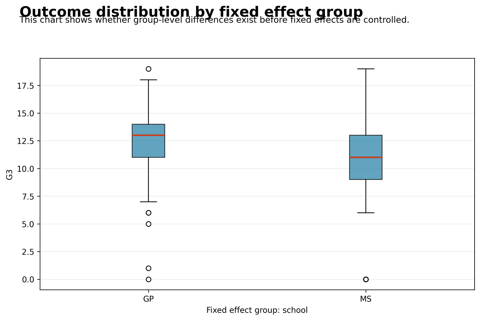
G3 has N = 649, mean 11.9060, median 12, standard deviation 3.2307, first quartile 10, third quartile 14, minimum 0 and maximum 19. The most frequent score is 11 with 104 records, followed by 10 with 97, 13 with 82, 12 with 72 and 14 with 63.
The outcome is bounded and integer valued, with a dense middle and a smaller low-grade tail. Ordinary least squares treats the conditional mean as continuous. The large sample supports mean-model estimation, but residual diagnostics remain necessary because zero scores create several unusually large negative residuals.
Python Chart 2: Observed vs Fitted G3
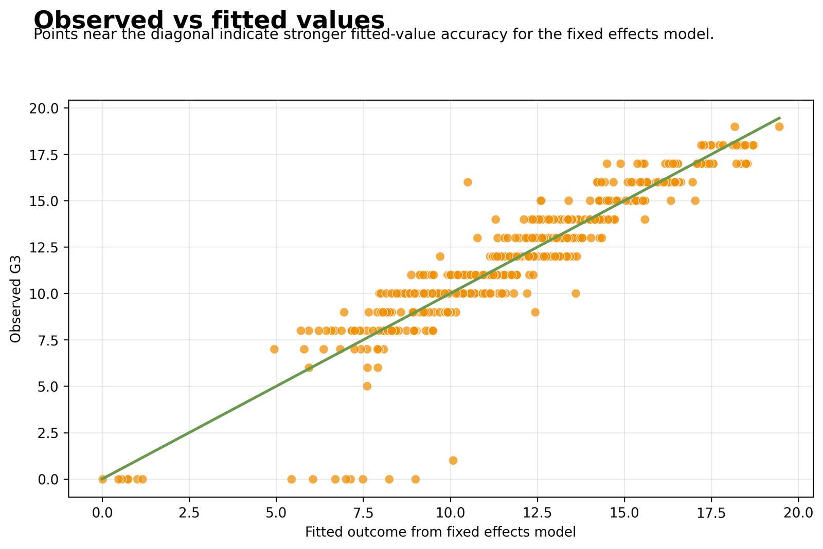
The correlation between observed and fitted G3 is 0.923392. Fitted values range from approximately 0.0119 to 19.4504. The model’s RMSE is 1.2392 and MAE is 0.7774. Most points lie close to the 45-degree line, particularly through the central grade range.
The largest deviations occur for unusually low observed outcomes. One record has G3 = 1 but a fitted value of 10.0753, producing a residual of -9.0753. Another has G3 = 0 and fitted value 8.9991. These cases explain why strong R² can coexist with important individual prediction errors.
Python Chart 3: Residuals vs Fitted Values
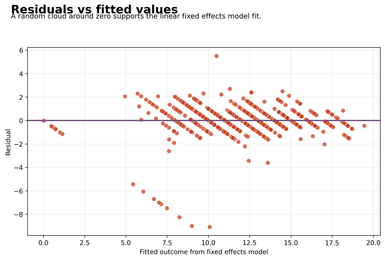
The residual mean is essentially 0, the residual SD is 1.2401, and the median is -0.0139. The middle 50% ranges from -0.4803 to 0.6475. The full range is asymmetric, from -9.0753 to 5.5036.
The negative tail is driven by zero or very low G3 observations that the model predicts substantially higher. Adjusted R² does not test homoskedasticity, normality or influence. Review studentized residuals, Q-Q plots, Cook’s distance and robust standard errors before describing assumptions as satisfactory.
Python Chart 4: Adjusted R Squared Model Comparison
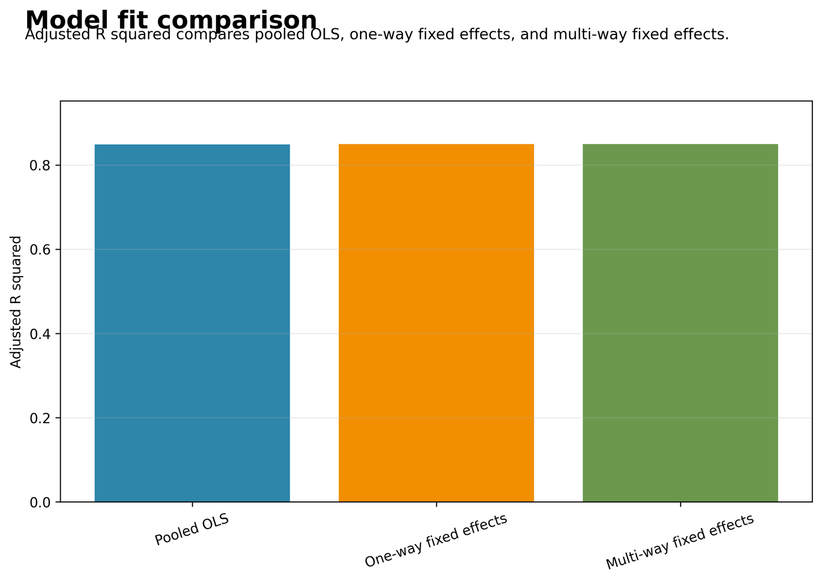
Adjusted R² is 0.848912 for pooled OLS, 0.849315 for one-way fixed effects and 0.849872 for multi-way fixed effects. The one-way gain over pooled OLS is only 0.000403. The multi-way gain over one-way is 0.000557, and its gain over pooled OLS is 0.000960.
The chart identifies the largest adjusted R² but not statistical significance. The corresponding nested F-test p-values are .1000, .1479 and .0896. Therefore, the chart supports a small incremental fit advantage, not strong evidence that all fixed-effect additions are necessary.
Python Chart 5: Fixed-Effect Group Means
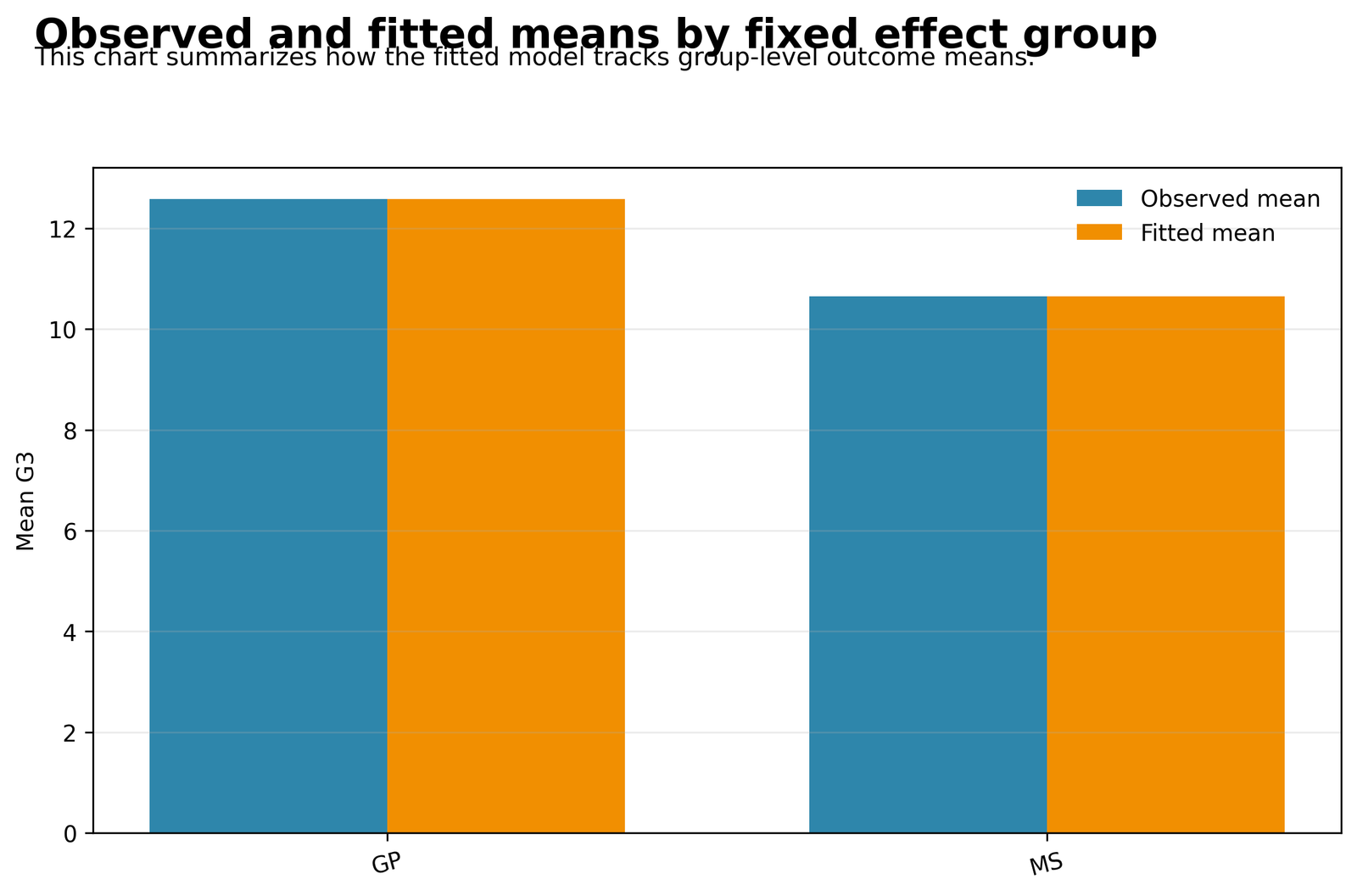
School means are 12.5768 for GP (n = 423) and 10.6504 for MS (n = 226). Sex means are 12.2533 for F and 11.4060 for M. Address means are 11.0863 for R and 12.2633 for U. Higher-education intention means are 8.7971 for no and 12.2759 for yes.
These are unadjusted descriptive means. Their gaps are much larger than the regression dummy coefficients because G1, G2, failures and other numeric predictors differ across groups. The chart should therefore be followed by the adjusted group-coefficient chart rather than interpreted as causal group effects.
Python Chart 6: Numeric Predictor Coefficients
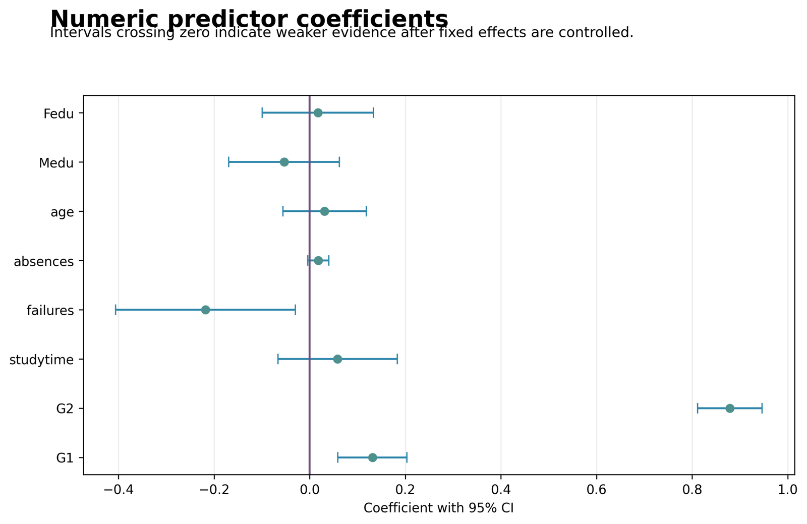
G2 is the dominant positive coefficient at 0.8792, 95% CI [0.8117, 0.9466]. G1 is 0.1313, CI [0.0588, 0.2037]. Failures is -0.2178, CI [-0.4060, -0.0297]. These three intervals exclude zero.
Studytime = 0.0584, absences = 0.0182, age = 0.0311, Medu = -0.0536 and Fedu = 0.0171 all have intervals crossing zero. The chart shows effect size and uncertainty; the large G2 t value of 25.6035 explains most of the model’s high fit.
Python Chart 7: Within-Transformed G2–G3 Relationship
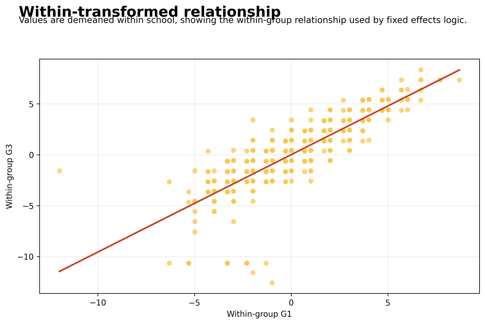
After demeaning G2 and G3 within school × sex × address × higher cells, the correlation is 0.902094. The simple within slope is 0.987075. Demeaned G2 ranges from approximately -11.2687 to 7.1176, while demeaned G3 ranges from -11.5970 to 7.7941.
The positive within relationship shows that students with G2 above their fixed-cell mean also tend to have G3 above their fixed-cell mean. The full regression G2 coefficient is 0.8792 rather than 0.9871 because the model simultaneously controls G1 and the other numeric predictors.
Python Chart 8: Fixed-Effect Group Coefficients
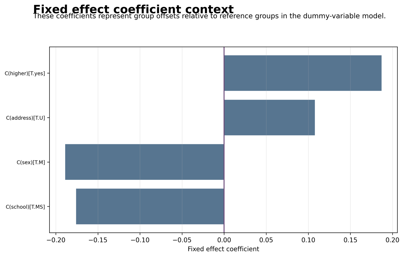
The adjusted coefficients are school_MS = -0.1759, sex_M = -0.1887, address_U = 0.1077 and higher_yes = 0.1870. Their p-values are .1405, .0717, .3500 and .2978, respectively.
Every 95% interval crosses zero. The closest to conventional significance is sex_M, with interval [-0.3942, 0.0167]. The chart demonstrates how large raw group mean gaps can become small after prior academic performance and other numeric terms are controlled.
R Charts, Tables and Independent Validation
The supplied media list repeats the same URLs for charts 01 through 07 and provides a distinct -1 URL for chart 08. The R section therefore uses those supplied assets and validates the workbook results. Separate R URLs should replace repeated assets later if WordPress created distinct media files.
Open the expected Fixed Effects Regression R report PDF
R Consolidated Model-Fit Table
| R Specification | N | R² | Adjusted R² | RMSE | MAE | AIC | BIC |
|---|---|---|---|---|---|---|---|
| Pooled numeric model | 649 | 0.850777 | 0.848912 | 1.247020 | 0.780019 | 2146.3247 | 2186.6036 |
| School fixed effects | 649 | 0.851408 | 0.849315 | 1.244381 | 0.778888 | 2145.5751 | 2190.3294 |
| School + sex + address + higher | 649 | 0.852652 | 0.849872 | 1.239162 | 0.777422 | 2146.1196 | 2204.3002 |
R Chart 1: Outcome Distribution Validation
R uses the same outcome with mean 11.9060, median 12, SD 3.2307 and range 0 to 19. The central mass between 10 and 14 and the low zero-score tail must be reproduced in any R diagnostic report.
R Chart 2: Observed vs Fitted Validation
The observed–fitted correlation is approximately 0.9234, with RMSE 1.2392 and MAE 0.7774. The R interpretation should emphasize strong aggregate fit and the same extreme low-grade overpredictions identified in Python.
R Chart 3: Residual Diagnostic Validation
The residual mean is effectively zero, but the range from -9.0753 to 5.5036 is asymmetric. The R workflow should supplement this figure with Q-Q, influence and heteroskedasticity checks rather than treating adjusted R² as an assumption test.
R Chart 4: Adjusted R Squared Comparison Validation
R reproduces the sequence .848912, .849315 and .849872. The difference between the highest and lowest value is less than .001, so model-selection discussion must include nested tests and information criteria.
R Chart 5: Group Means Validation
The R chart should reproduce the GP/MS, F/M, R/U and no/yes mean differences. The largest raw gap is higher=yes versus higher=no, 12.2759 versus 8.7971, but the adjusted higher_yes coefficient is only 0.1870.
R Chart 6: Numeric Coefficient Validation
R confirms the three intervals away from zero: G2 0.8792, G1 0.1313 and failures -0.2178. The remaining numeric predictors have confidence intervals that include zero.
R Chart 7: Within-Transformed Relationship Validation
The transformed relationship has correlation approximately 0.9021 and simple slope approximately 0.9871. It provides a visual explanation of within-group adjustment but is not a replacement for the complete multivariable coefficient table.
R Chart 8: Fixed-Effect Coefficient Validation
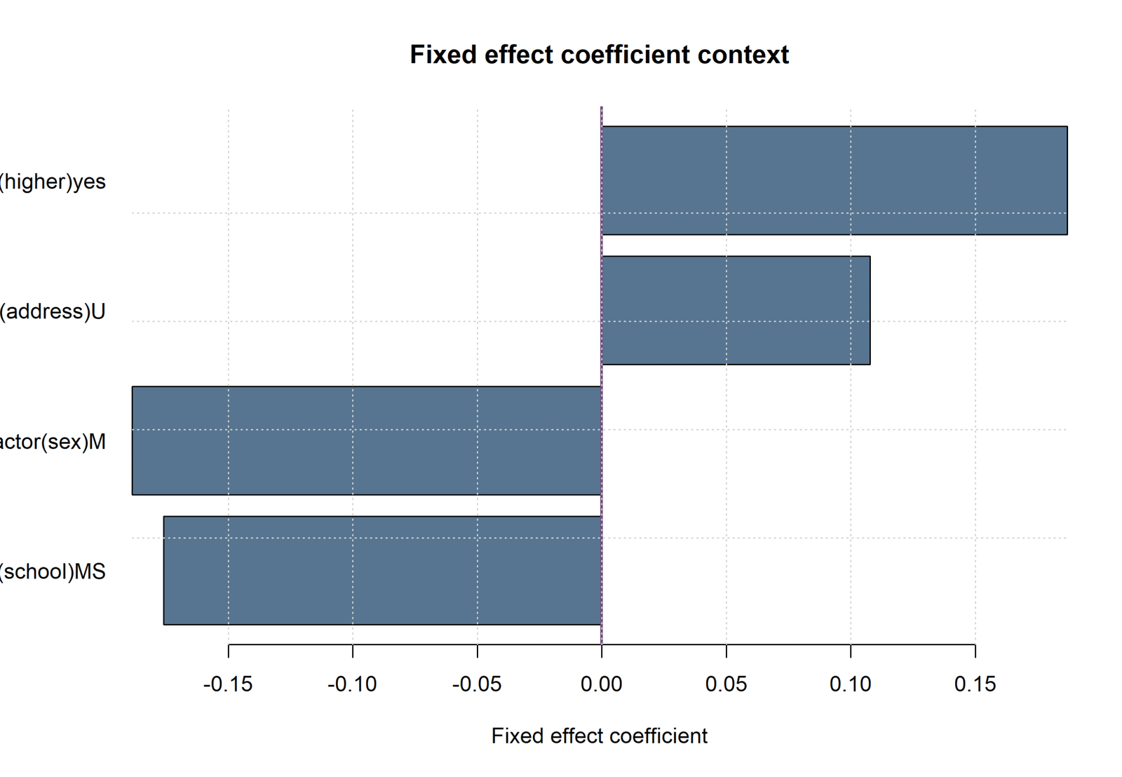
The R chart validates the four adjusted group terms: -0.1759 for school_MS, -0.1887 for sex_M, 0.1077 for address_U and 0.1870 for higher_yes. None has a 95% interval fully away from zero.
R validation conclusion: the substantive result is driven by G2, G1 and failures. Adding the named fixed effects produces a small adjusted-R² improvement but no significant nested-model improvement at .05.
SPSS Fixed Effects Regression Output Interpretation
The confirmed SPSS output is available at the Cox-independent Fixed Effects Regression PDF link below. The unrelated Elastic Net SPSS PDF is not used.
Open the Fixed Effects Regression SPSS output PDF
In SPSS, fixed group effects can be represented through dummy variables in REGRESSION, categorical factors in UNIANOVA/GLM or repeated/panel structures in procedures appropriate to the design. For the workbook specification, the simplest equivalent is ordinary linear regression with four dummy variables and eight numeric predictors.
| SPSS Output | What to Check | Interpretation |
|---|---|---|
| Model Summary | R, R Square, Adjusted R Square and Std. Error | Compare pooled and fixed-effect specifications using the same complete cases. |
| ANOVA table | Overall F and Sig. | Tests whether the complete predictor set improves on an intercept-only model. |
| Coefficients table | B, SE, Beta, t, Sig. and confidence intervals | Use unstandardized B for outcome-unit interpretation. |
| Dummy variables | Reference coding | Confirm GP, F, R and no are omitted categories. |
| Collinearity statistics | Tolerance and VIF | Identify redundancy between numeric predictors and group indicators. |
| Residual plots | Linearity, variance and influential observations | Do not infer assumptions from R² alone. |
| Change statistics | R² change and F change | Enter fixed-effect blocks hierarchically to test incremental fit. |
SPSS file rule: use only Fixed-Effects-Regression-SPSS-Output.pdf for this article. Elastic-Net-Regression-SPSS-Output.pdf belongs to the separate Elastic Net Regression post.
Excel Worked Fixed Effects Regression Results
The workbook contains the complete 649-row model, formula-driven fitted values and residuals, model summaries, coefficients, group summaries and nested F tests. It is not a small demonstration workbook; it directly reproduces the full multi-way model results.
Excel Model Summary
| Metric | Excel Value | Interpretation |
|---|---|---|
| N | 649 | Complete observations used. |
| Parameters excluding intercept | 12 | Eight numeric terms and four fixed-effect dummies. |
| SSE | 996.5545 | Residual squared error. |
| SST | 6763.2666 | Total outcome variation around the mean. |
| R² | 0.852652 | 85.27% of sample G3 variance explained. |
| Adjusted R² | 0.849872 | Fit after accounting for 12 slope parameters. |
| RMSE | 1.239162 | Root mean squared prediction error. |
| MAE | 0.777422 | Mean absolute prediction error. |
Excel Prediction Formula
For each row, the workbook creates four dummy variables: school_MS, sex_M, address_U and higher_yes. The fitted-value formula multiplies each data value by its corresponding coefficient. Residual equals observed G3 minus predicted G3. Squared residuals sum to SSE, while deviations from the outcome mean sum to SST.
Core Excel Formulas
| Quantity | Excel Formula Pattern | Purpose |
|---|---|---|
| Dummy variable | =--(school_cell="MS") | Convert category membership into 1/0 coding. |
| Predicted value | =Intercept + SUMPRODUCT(row_predictors, coefficient_range) | Generate fitted G3. |
| Residual | =Observed_G3-Predicted_G3 | Calculate row error. |
| SSE | =SUM(squared_residual_range) | Total unexplained squared variation. |
| SST | =DEVSQ(observed_G3_range) | Total squared variation around the observed mean. |
| R² | =1-SSE/SST | Explained proportion of variance. |
| Adjusted R² | =1-(1-R2)*(N-1)/(N-k-1) | Penalize fit for slope count. |
| RMSE | =SQRT(SSE/N) | Prediction error on the G3 scale. |
| MAE | =AVERAGE(absolute_residual_range) | Average absolute error. |
Nested F-Test Formula
Here, q is the number of added fixed-effect parameters. The workbook reports p = .0896 for adding all four fixed effects to pooled OLS, so the expanded model is not significant at .05 under the nested F test.
Python, R, SPSS and Excel Workflows
| Software | Main Method | Outputs | Best Use |
|---|---|---|---|
| Python | statsmodels formula OLS with C(group) dummy coding and nested-model comparisons. | Eight PNG charts, CSV tables, TXT and PDF report. | Automated reporting and diagnostic chart generation. |
| R | lm() with factor terms; optionally plm or fixest for true panel/high-dimensional FE. | Charts, tables, nested tests, TXT and PDF report. | Panel methods, robust covariance and within-estimator validation. |
| SPSS | REGRESSION with prepared dummies or GLM/UNIANOVA categorical factors. | SAV, SPV, PDF and standard diagnostic output. | GUI-compatible reporting and hierarchical block tests. |
| Excel | Formula-driven fitted values and summary metrics using imported coefficients. | Full worked workbook with 649 rows. | Transparent calculations and instructional review. |
Fixed Effects Regression Code
Python Code
import pandas as pd
import statsmodels.formula.api as smf
from statsmodels.stats.anova import anova_lm

df = pd.read_csv("dataset.csv")

numeric = [
    "G1", "G2", "studytime", "failures",
    "absences", "age", "Medu", "Fedu"
]
required = ["G3", *numeric, "school", "sex", "address", "higher"]
work = df[required].dropna().copy()

pooled_formula = "G3 ~ " + " + ".join(numeric)
one_way_formula = pooled_formula + " + C(school)"
multi_way_formula = (
    pooled_formula
    + " + C(school) + C(sex) + C(address) + C(higher)"
)

pooled = smf.ols(pooled_formula, data=work).fit()
one_way = smf.ols(one_way_formula, data=work).fit()
multi_way = smf.ols(multi_way_formula, data=work).fit()

print(multi_way.summary())
print(anova_lm(pooled, one_way))
print(anova_lm(one_way, multi_way))
print(anova_lm(pooled, multi_way))

# Heteroskedasticity-robust covariance
multi_way_hc3 = multi_way.get_robustcov_results(cov_type="HC3")
print(multi_way_hc3.summary())
R Code
df <- read.csv("dataset.csv", stringsAsFactors = TRUE)

numeric_terms <- c(
  "G1", "G2", "studytime", "failures",
  "absences", "age", "Medu", "Fedu"
)

pooled <- lm(
  G3 ~ G1 + G2 + studytime + failures +
    absences + age + Medu + Fedu,
  data = df
)

one_way <- update(pooled, . ~ . + school)

multi_way <- update(
  pooled,
  . ~ . + school + sex + address + higher
)

summary(multi_way)
anova(pooled, one_way)
anova(one_way, multi_way)
anova(pooled, multi_way)

# Robust standard errors
library(sandwich)
library(lmtest)
coeftest(multi_way, vcov = vcovHC(multi_way, type = "HC3"))

# For true panel data:
# library(fixest)
# feols(y ~ x1 + x2 | entity + year, data = panel_df)
SPSS Syntax Pattern
* Prepare reference-coded fixed-effect dummies.
COMPUTE school_MS = (school = 'MS').
COMPUTE sex_M = (sex = 'M').
COMPUTE address_U = (address = 'U').
COMPUTE higher_yes = (higher = 'yes').
EXECUTE.

REGRESSION
  /DEPENDENT G3
  /METHOD=ENTER G1 G2 studytime failures absences age Medu Fedu
  /METHOD=ENTER school_MS sex_M address_U higher_yes
  /STATISTICS COEFF OUTS R ANOVA CHANGE CI(95) COLLIN TOL
  /RESIDUALS HISTOGRAM(ZRESID) NORMPROB(ZRESID)
  /SAVE PRED RESID ZRESID COOK LEVER.

OUTPUT SAVE OUTFILE=
'D:\DATA ANALYSIS\H Regression Tests and Models\Fixed Effects Regression\SPSS_Output\spv\Fixed-Effects-Regression-SPSS-Output.spv'.

OUTPUT EXPORT
  /CONTENTS EXPORT=ALL LAYERS=PRINTSETTING MODELVIEWS=PRINTSETTING
  /PDF DOCUMENTFILE=
'D:\DATA ANALYSIS\H Regression Tests and Models\Fixed Effects Regression\SPSS_Output\pdf\Fixed-Effects-Regression-SPSS-Output.pdf'.
Excel Formula Pattern
Dummy variables:
=--(J2="MS")
=--(K2="M")
=--(L2="U")
=--(M2="yes")

Predicted fixed-effects value:
=$B$intercept
 + G1*$B$G1
 + G2*$B$G2
 + studytime*$B$studytime
 + failures*$B$failures
 + absences*$B$absences
 + age*$B$age
 + Medu*$B$Medu
 + Fedu*$B$Fedu
 + dummy_school_MS*$B$school_MS
 + dummy_sex_M*$B$sex_M
 + dummy_address_U*$B$address_U
 + dummy_higher_yes*$B$higher_yes
Robust and Clustered Standard Errors
Fixed effects change the conditional mean specification; they do not automatically correct the covariance matrix. Cross-sectional heteroskedasticity can make conventional standard errors unreliable. HC3 robust standard errors are often useful for ordinary dummy-variable regression.
In true panel data, observations from the same entity are usually correlated over time. Standard errors should generally be clustered at the entity level. When treatment or policy varies at a higher aggregation level, clustering may need to match the assignment level.
| Error Structure | Recommended Covariance | Example |
|---|---|---|
| Heteroskedastic independent observations | HC2 or HC3 robust | Cross-sectional student data. |
| Repeated observations within entity | Cluster by entity | Students observed across semesters. |
| Common shocks within year | Two-way cluster by entity and year where supported | Firms observed across macroeconomic years. |
| Few clusters | Small-sample cluster corrections or wild bootstrap | Only a small number of schools. |
| Serial and cross-sectional dependence | Design-specific panel covariance | Long country panels. |
Coefficient values remain the same when only the covariance estimator changes, but standard errors, confidence intervals and p-values can change materially. Always report the covariance method.
APA-Style Reporting for Fixed Effects Regression
Full Multi-Way Model Report
A multi-way fixed-effects regression was fitted to predict G3 final grade from G1, G2, studytime, failures, absences, age, maternal education and paternal education while controlling fixed intercept differences for school, sex, address and higher-education intention. The model used 649 complete observations and explained 85.27% of the sample variance, R² = .853, adjusted R² = .850, RMSE = 1.239, and MAE = 0.777. G2 was the strongest positive predictor, B = 0.879, 95% CI [0.812, 0.947], p < .001. G1 was also positive, B = 0.131, 95% CI [0.059, 0.204], p < .001, whereas previous failures was negative, B = -0.218, 95% CI [-0.406, -0.030], p = .023. None of the four fixed-effect dummy coefficients was statistically significant at alpha .05.
Model-Comparison Report
Adjusted R² increased from .8489 for pooled OLS to .8493 for one-way school fixed effects and .8499 for the multi-way fixed-effects model. However, adding all four fixed-effect dummies did not significantly improve fit over pooled OLS, F(4, 636) = 2.023, p = .090. The one-way model had the lowest AIC, whereas pooled OLS had the lowest BIC.
Short Results Version
The multi-way fixed-effects model achieved adjusted R² = .850, but its improvement over pooled OLS was not significant at .05. G2 and G1 were positive adjusted predictors of G3, and failures was negative. The fixed-effect group coefficients were not statistically significant after academic and background variables were controlled.
Fixed Effects Regression Reporting Checklist
| Reporting Item | What to Include | Reason |
|---|---|---|
| Data structure | Cross-sectional or panel, number of entities, periods and observations. | Determines what “fixed effects” means. |
| Outcome | Name, units and distribution. | Makes coefficients interpretable. |
| Numeric predictors | Names, scaling and transformations. | Clarifies one-unit effects. |
| Fixed-effect dimensions | School, entity, year or other groups. | Defines what stable differences are controlled. |
| Reference categories | Omitted levels for dummy-variable models. | Required for group-coefficient interpretation. |
| Estimation method | LSDV, within estimator, absorbed FE or high-dimensional FE. | Supports reproducibility. |
| Covariance method | Classical, HC3, clustered or multi-way clustered. | Determines inferential uncertainty. |
| Fit statistics | R², within R², adjusted R², RMSE, AIC/BIC as appropriate. | Different metrics answer different questions. |
| Nested tests | F test or likelihood comparison for added fixed effects. | Evaluates incremental fit. |
| Diagnostics | Residual, leverage, influence and collinearity checks. | Protects against misleading high fit. |
| Limitations | Remaining time-varying confounding and design limitations. | Prevents causal overclaiming. |
Common Fixed Effects Regression Mistakes
| Mistake | Why It Is Wrong | Better Practice |
|---|---|---|
| Calling any categorical dummy a panel entity fixed effect | Panel FE requires repeated observations and within-entity interpretation. | State whether the model is cross-sectional LSDV or repeated panel FE. |
| Including every category dummy plus an intercept | Creates perfect multicollinearity. | Omit one reference category or omit the global intercept. |
| Interpreting raw group means as adjusted coefficients | They answer different questions. | Report descriptive means and conditional coefficients separately. |
| Selecting the largest adjusted R² automatically | The gain may be tiny and statistically unsupported. | Use nested tests, AIC/BIC, prediction and theory. |
| Using ordinary SEs for repeated panel observations | Within-entity dependence can understate uncertainty. | Cluster at the appropriate level. |
| Estimating a time-invariant predictor with entity FE | It is collinear with the entity effects. | Use a different design or estimator when that effect is the target. |
| Assuming fixed effects solve all confounding | Time-varying omitted variables remain possible. | Use research design, controls, instruments or sensitivity analysis. |
| Using the Elastic Net SPSS PDF in this post | It belongs to a penalized-regression analysis. | Use only the confirmed Fixed Effects Regression SPSS output. |
Fixed Effects Regression Troubleshooting Guide
Dummy Variable Is Automatically Dropped
The dropped term is usually the reference category or is perfectly collinear with another variable. Inspect the design matrix and coding. One level per categorical fixed effect must be omitted when an intercept is included.
Time-Invariant Predictor Disappears in Panel FE
This is expected. Entity demeaning removes every variable that does not change within the entity. The effect cannot be separated from the entity fixed intercept without additional assumptions or a different design.
Adjusted R Squared Barely Changes
The added fixed effects may explain little residual variation after the numeric predictors are included. In this workbook, adjusted R² increases by less than .001 from pooled to multi-way fixed effects. Report the small gain accurately.
Raw Group Difference Is Large but Dummy Coefficient Is Small
The covariates explain much of the raw difference. Higher=yes students average 3.4788 points above higher=no students, but the adjusted coefficient is only 0.1870 because prior grades and other predictors differ strongly across the groups.
Python, R and SPSS Coefficients Differ
Check complete-case rows, category reference levels, contrast coding, predictor lists, transformations and covariance estimators. Dummy-label differences such as C(school)[T.MS] versus schoolMS are naming differences when coding is otherwise identical.
High R Squared but Poor Residual Tail
G1 and G2 make prediction strong overall, but several zero-score observations have residuals below -7. High R² does not eliminate outliers or influence. Review case-level diagnostics and sensitivity analyses.
Too Many Fixed Effects
High-dimensional fixed effects can consume degrees of freedom and memory. Use within/absorption algorithms such as fixest, lfe or specialized panel estimators rather than explicitly creating thousands of dummy columns.
Nested F Test Is Not Significant
Keep or remove fixed effects based on the estimand, design and confounding logic—not only one threshold. A theoretically required entity or time effect may remain in the model even when its joint incremental test is modest.
Downloads and Resources
Media verification: the Python and SPSS links are confirmed from the supplied URLs. The R report and hosted Excel links use expected filenames and should be checked in WordPress Media. The Elastic Net SPSS PDF is excluded.
R Fixed Effects Report PDFExpected R report filename; verify the final Media Library URL.
SPSS Fixed Effects Output PDFConfirmed Fixed Effects Regression SPSS output.
Worked Excel FileExpected hosted filename for the 649-row formula-driven workbook.
FAQs About Fixed Effects Regression
What is fixed effects regression?
It is a regression approach that controls group-specific intercept differences through dummy variables, demeaning or absorbed fixed effects.
What outcome and predictors were used?
G3 was predicted from G1, G2, studytime, failures, absences, age, Medu and Fedu, with fixed effects for school, sex, address and higher-education intention.
What was the best adjusted R squared?
The multi-way fixed-effects model had adjusted R² = 0.849872.
Did fixed effects significantly improve pooled OLS?
No. Adding all four fixed effects produced F = 2.0229 with p = 0.0896, which is not significant at .05.
Which predictors were statistically significant?
G2 and G1 were positive, while failures was negative. None of the four fixed-effect dummy coefficients was significant at .05.
Why are raw group means different from adjusted coefficients?
Raw means include differences in prior grades and other covariates. Adjusted fixed-effect coefficients compare groups after those variables are controlled.
Is this a panel fixed-effects model?
The workbook is a cross-sectional least-squares dummy-variable model. A true entity panel fixed-effects model requires repeated observations within entities.
What is the within transformation?
It subtracts group means from the outcome and time-varying predictors, removing group-specific intercepts from the estimating equation.
Can time-invariant variables be estimated with entity fixed effects?
No. They are perfectly collinear with entity fixed effects and disappear under within transformation.
How are fixed effects added in SPSS?
Create reference-coded dummy variables or use a categorical-factor procedure, then enter the fixed-effect block after the numeric predictors to obtain R²-change and F-change results.
How are fixed effects fitted in R?
Use lm() with factor variables for modest dummy sets, or packages such as fixest for high-dimensional entity and time fixed effects.
How are fixed effects fitted in Python?
Use statsmodels formulas with C(group) for dummy-variable fixed effects, or panel-specific libraries when repeated entity-time data are available.
Can Excel estimate fixed effects?
Excel can calculate dummy-variable predictions and summaries. Formal coefficient estimation can use LINEST for modest models, although Python, R or SPSS is easier for large categorical specifications and diagnostics.
Should fixed or random effects be used?
The choice depends on the estimand and whether group effects plausibly correlate with predictors. Fixed effects are robust to that correlation but do not estimate time-invariant predictor effects under entity FE.
Final Fixed Effects Regression Conclusion
The multi-way fixed-effects model explains 85.27% of G3 variance and has adjusted R² = 0.849872. Its fitted values correlate 0.923392 with observed G3. G2 is the dominant adjusted predictor, followed by G1, while previous failures has a smaller negative effect.
The fixed-effect group dummies add only a small amount of model fit after the numeric predictors are included. Their joint improvement over pooled OLS is not significant at .05, and none of the four individual dummy intervals excludes zero. The results support strong academic prediction but limited incremental evidence for the named group intercept shifts in this specification.
The most accurate final report distinguishes raw group means from adjusted effects, states the reference categories, reports the nested tests and information criteria, checks residual and influence diagnostics, and avoids treating a cross-sectional dummy-variable model as automatically equivalent to a repeated panel fixed-effects design.

