
Correlation, Control Variables, Residual Analysis and Excel Worked Results
Partial Correlation: Formula, Interpretation, SPSS, Python, R and Excel Guide
Partial Correlation measures the relationship between two variables after removing the influence of one or more control variables. This complete guide explains zero-order correlation, partial correlation, semi-partial correlation, the formula, assumptions, SPSS output interpretation, Python chart interpretation, R validation charts, Excel worked formulas, APA reporting wording, common mistakes, internal resources and downloadable files.
Quick Answer: Partial Correlation Result
The main SPSS, Python, R and Excel report tested the association between G1 first-period grade and G3 final grade while controlling G2 second-period grade. The sample contained N = 649 complete cases. Before controlling G2, the zero-order correlation between G1 and G3 was very strong, r = 0.8264.
After the shared influence of G2 was removed, the partial correlation between G1 and G3 dropped to r = 0.1606. The test statistic was t(646) = 4.1359, with a two-tailed p = 0.000040. The relationship remained statistically significant, but the practical interpretation changed from a very strong raw relationship to a small adjusted relationship.
Final interpretation: G1 and G3 have a very strong raw relationship, but most of that relationship is shared with G2. After controlling G2, G1 still explains a small but statistically significant unique part of G3.
Important distinction: A zero-order correlation answers “Are G1 and G3 related?” A partial correlation answers “Are G1 and G3 still related after G2 is held constant?” In this example, the answer changes because G2 is highly connected to both G1 and G3.
Table of Contents
- What Is Partial Correlation?
- Zero-Order vs Partial vs Semi-Partial Correlation
- Partial Correlation Formula
- Null and Alternative Hypotheses
- Dataset and Variables Used
- SPSS Output Interpretation
- Python Chart-by-Chart Interpretation
- R Chart-by-Chart Validation
- Excel Results Explained
- SPSS, R, Python and Excel Workflows
- Code Blocks for Partial Correlation
- APA Reporting Wording
- Common Mistakes
- When to Use Partial Correlation
- Downloads and Resources
- Related Guides
- FAQs
What Is Partial Correlation?
Partial correlation is a correlation coefficient that measures the relationship between two variables after one or more other variables have been statistically controlled. It is useful when a simple correlation may be inflated because both variables are connected to a third variable.
In the worked example, G1 and G3 are strongly correlated before any adjustment. That makes sense because a student who performs well early in a course often performs well at the final stage too. However, G2 sits between them as a very strong related grade variable. Partial correlation removes the part of G1 and G3 that is predictable from G2, then correlates the remaining residual parts.
Because partial correlation is based on adjusted residual relationships, it is often used in education, psychology, health research, economics and social science. It helps the researcher ask whether an association is still present after a specific control variable is held constant.
Simple definition: Partial correlation is the correlation between the leftover part of X and the leftover part of Y after the control variable has been removed from both.
Zero-Order vs Partial vs Semi-Partial Correlation
Students often confuse zero-order correlation, partial correlation and semi-partial correlation. The difference is based on how the control variable is removed.
| Coefficient | Use It When | Example | Main Interpretation |
|---|---|---|---|
| Zero-order correlation | No control variable is removed. | Correlation between G1 and G3. | Shows the raw relationship before adjustment. |
| Partial correlation | The control variable is removed from both X and Y. | G1 and G3 controlling G2. | Shows the adjusted relationship between the residual part of X and residual part of Y. |
| Semi-partial correlation | The control variable is removed from only one variable. | G3 with G1 after removing G2 from G1 only. | Shows the unique contribution of one predictor to an outcome. |
| Multiple correlation | Several predictors jointly predict one outcome. | G1 and G2 predicting G3. | Shows the combined relationship between predictors and the outcome. |
Better reporting rule: Do not report a partial correlation as if it were an ordinary correlation. Always state the control variable, because the coefficient can change dramatically after statistical control.
Partial Correlation Formula
When there is one control variable, the partial correlation formula uses three ordinary Pearson correlations: the correlation between X and Y, the correlation between X and Z, and the correlation between Y and Z.
| Symbol | Meaning | Value in This Example |
|---|---|---|
| rxy | Zero-order correlation between G1 and G3 | 0.8264 |
| rxz | Zero-order correlation between G1 and G2 | 0.8650 |
| ryz | Zero-order correlation between G3 and G2 | 0.9185 |
| rxy.z | Partial correlation between G1 and G3 controlling G2 | 0.1606 |
| n | Number of complete observations | 649 |
| k | Number of control variables | 1 |
| df | Degrees of freedom, n − k − 2 | 646 |
The significance test for a partial correlation uses this t statistic:
For the main result, this gives t(646) = 4.1359 and p = 0.000040. The result is statistically significant, but the adjusted coefficient is small compared with the original zero-order correlation.
Null and Alternative Hypotheses for Partial Correlation
The hypothesis statement should name the two main variables and the control variable. In this guide, the main question is whether G1 and G3 remain related after controlling G2.
| Statement | Hypothesis | Meaning |
|---|---|---|
| Null hypothesis | H0: ρG1,G3.G2 = 0 | After controlling G2, G1 and G3 have no linear association in the population. |
| Alternative hypothesis | H1: ρG1,G3.G2 ≠ 0 | After controlling G2, G1 and G3 are still associated in the population. |
| Decision rule | Reject H0 if p < .05 | Use the two-tailed p-value from the partial correlation test. |
Decision for the main report: Because p = 0.000040 is below .05, the null hypothesis is rejected. G1 and G3 retain a statistically significant adjusted relationship after G2 is controlled, although the adjusted effect is small.
Dataset and Variables Used
The worked example uses the student performance dataset. The main pair is G1 and G3, and the control variable is G2. The logic is educationally meaningful: G1 is the first-period grade, G2 is the second-period grade and G3 is the final grade.
| Variable | Role | N | Mean | Std. Dev. | Minimum | Maximum |
|---|---|---|---|---|---|---|
| G1 | X variable / first-period grade | 649 | 11.3991 | 2.7453 | 0 | 19 |
| G3 | Y variable / final grade | 649 | 11.9060 | 3.2307 | 0 | 19 |
| G2 | Control variable / second-period grade | 649 | 11.5701 | 2.9136 | 0 | 19 |
| age | Additional matrix variable | 649 | 16.7442 | 1.2181 | 15 | 22 |
| studytime | Additional matrix variable | 649 | 1.9307 | 0.8295 | 1 | 4 |
| failures | Additional matrix variable | 649 | 0.2219 | 0.5932 | 0 | 3 |
| absences | Additional matrix variable | 649 | 3.6595 | 4.6408 | 0 | 32 |
| Medu | Additional matrix variable | 649 | 2.5146 | 1.1346 | 0 | 4 |
| Fedu | Additional matrix variable | 649 | 2.3066 | 1.0999 | 0 | 4 |
Before interpreting the partial correlation, the dataset should be checked with descriptive statistics, correlation matrix, correlation heatmap, correlation assumptions, p-value, confidence interval and effect size guides.
SPSS Output Interpretation for Partial Correlation
The SPSS output should be read in two stages. First, the ordinary correlation matrix shows the raw relationship between G1 and G3. Second, the partial correlation table shows the adjusted relationship after G2 is controlled. The important change is the drop from r = 0.8264 to partial r = 0.1606.
Open the SPSS Partial Correlation output PDF
| SPSS Output Item | Value | Interpretation |
|---|---|---|
| Valid N | 649 | All complete cases for G1, G3 and G2 are included. |
| X variable | G1 | First-period grade, used as the main explanatory variable. |
| Y variable | G3 | Final grade, used as the main outcome variable. |
| Control variable | G2 | Second-period grade, removed from both G1 and G3. |
| Zero-order r(G1,G3) | 0.8264 | Very strong raw positive relationship before adjustment. |
| Partial r(G1,G3 controlling G2) | 0.1606 | Small positive adjusted relationship after controlling G2. |
| Degrees of freedom | 646 | Calculated as n − k − 2 with one control variable. |
| t statistic | 4.1359 | Positive test statistic because the adjusted relationship is positive. |
| Two-tailed p-value | 0.000040 | Statistically significant at alpha .05. |
| Decision | Significant partial relationship | Reject the null hypothesis, but report the effect as small. |
SPSS Interpretation Summary
The SPSS result means that G1 still has a statistically significant positive relationship with G3 after G2 is controlled. However, the effect is no longer large. This is the main substantive finding: the raw G1-G3 correlation is very strong, but most of it is explained by the grade progression captured by G2.
SPSS reporting note: In a formal report, write both the zero-order correlation and the partial correlation. This helps readers see how much the control variable changed the association.
Python Chart-by-Chart Interpretation
The Python charts show the full story visually: the strong zero-order relationship, the weaker residual relationship after controlling G2, the coefficient drop, the adjusted matrix, the strongest remaining adjusted pairs and the p-value summary.
Python Chart 1: Zero-Order Scatterplot
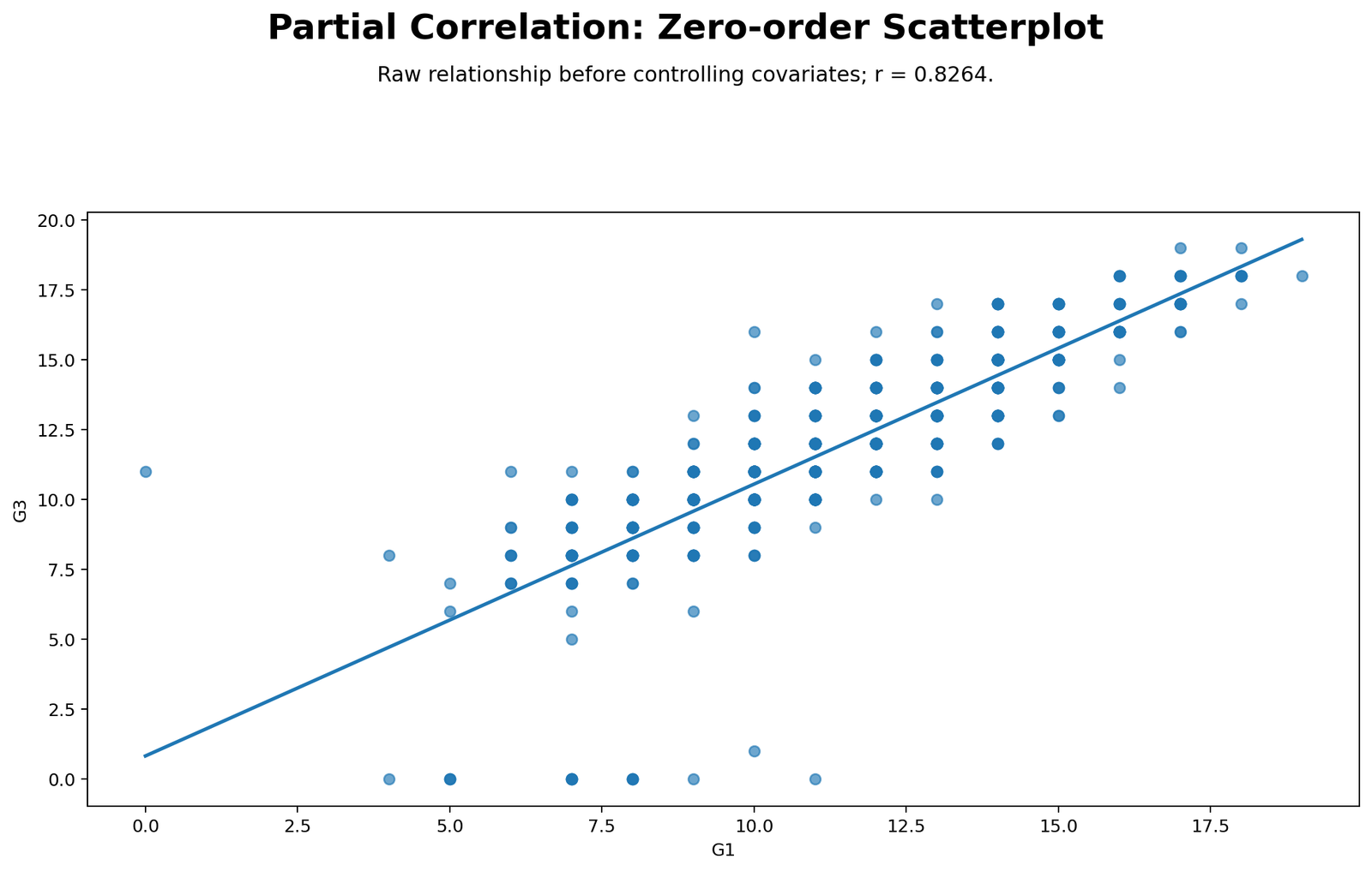
The zero-order scatterplot shows a strong positive relationship between G1 and G3. Students with higher G1 scores generally have higher G3 scores. This raw pattern explains why the zero-order correlation is very large at r = 0.8264.
This chart is important because it shows the relationship before statistical control. If the analysis stopped here, the report would conclude that G1 and G3 are strongly related. Partial correlation asks whether this relationship remains after G2 is removed.
Python Chart 2: Partial Residual Scatterplot
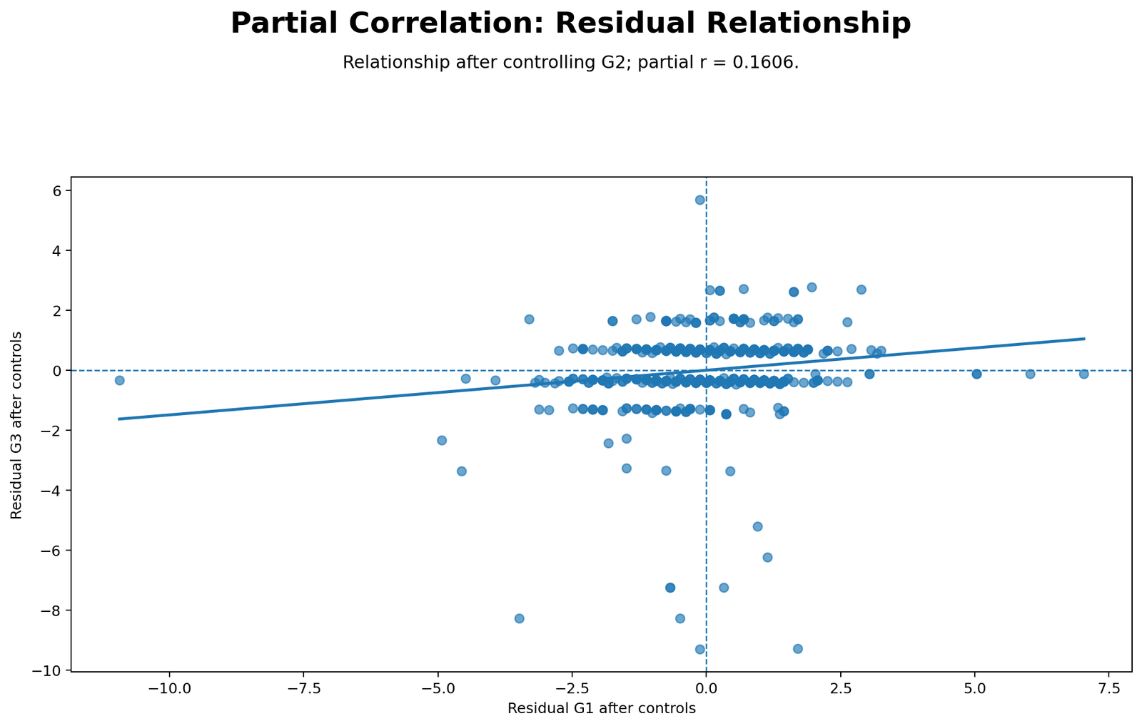
The residual scatterplot shows the relationship between the part of G1 not predicted by G2 and the part of G3 not predicted by G2. The positive trend is still visible, but it is much weaker than the raw scatterplot. This is why the partial correlation is only r = 0.1606.
The chart supports the final interpretation: G1 has a small unique relationship with G3 after G2 is held constant. The association is statistically significant because the sample is large, but the residual pattern is not strong.
Python Chart 3: Zero-Order vs Partial Correlation
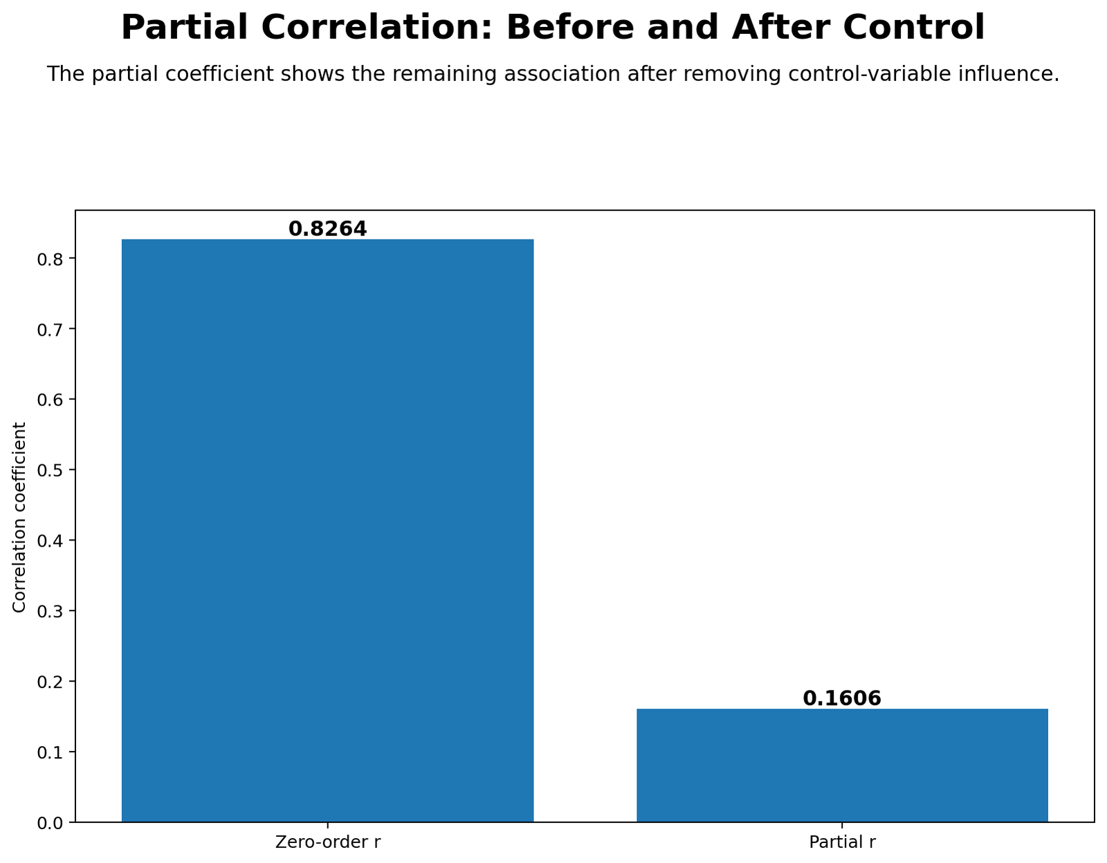
This chart makes the main result easy to understand. The zero-order correlation is 0.8264, while the partial correlation is 0.1606. The drop is large because G2 accounts for much of the shared relationship between G1 and G3.
The decision is not simply that the relationship “disappeared.” The adjusted relationship remains significant. The correct conclusion is that the original strong relationship becomes small once G2 is controlled.
Python Chart 4: Partial Correlation Heatmap
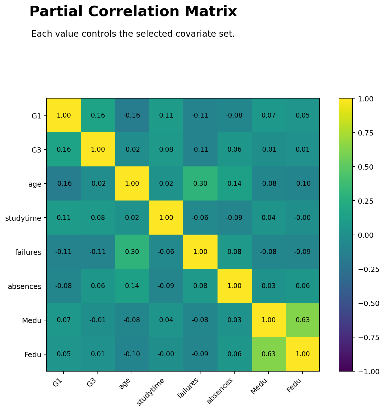
The heatmap displays adjusted correlations among several variables after controlling G2. The main G1-G3 cell is positive but modest at about 0.161. Other relationships remain stronger, especially the adjusted relationship between mother’s education and father’s education at about 0.626.
This chart shows that controlling G2 does not affect every relationship in the same way. Grade relationships involving G1 and G3 shrink strongly, while some background variables remain related after the same control variable is removed.
Python Chart 5: Largest Pairwise Partial Correlations
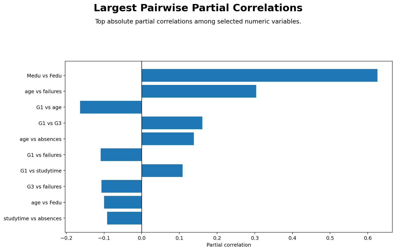
The ranking chart highlights the largest adjusted associations in the matrix. The strongest remaining relationship is Medu vs Fedu, around 0.626. Other notable adjusted relationships include age with failures, G1 with age, G1 with G3 and age with absences.
This chart provides context for the main result. The adjusted G1-G3 relationship is significant, but it is not the strongest relationship in the controlled matrix. It is better described as a small unique relationship rather than a dominant association.
Python Chart 6: Partial Correlation P-Values
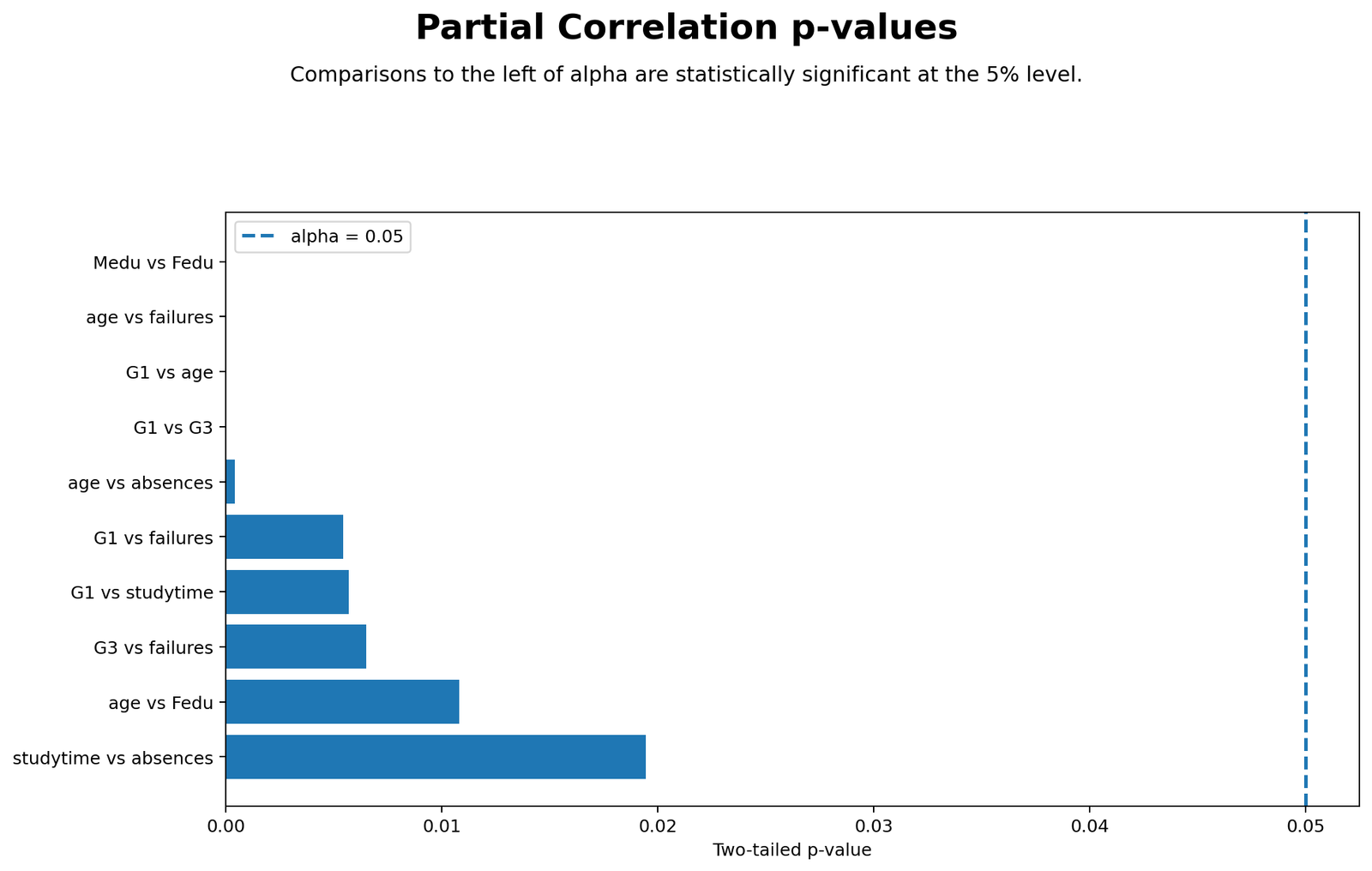
The p-value chart separates statistical significance from effect size. The G1-G3 partial correlation has p = 0.000040, so it is statistically significant. Some other adjusted relationships are not significant, such as G3 with age, which has p around 0.600.
This chart supports careful reporting. A small coefficient can be statistically significant when the sample is large, and a visually weak residual relationship can still pass the p-value test.
R Chart-by-Chart Validation
The R charts validate the same analysis using a separate workflow and colorful chart style. They repeat the zero-order view, residual view, coefficient comparison, heatmap, largest adjusted pairs and p-value display.
R Chart 1: Colorful Zero-Order Scatterplot
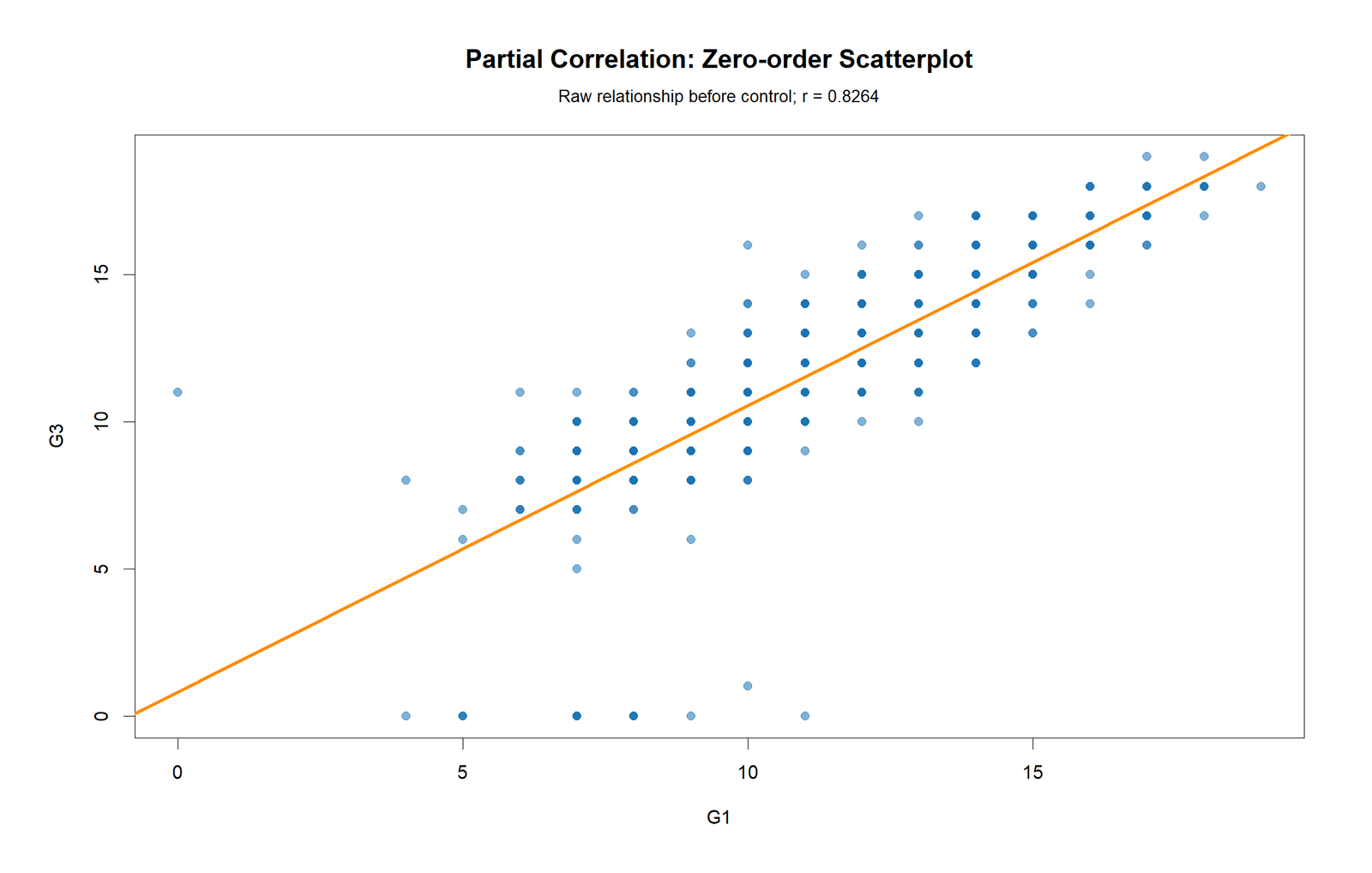
The R zero-order scatterplot confirms the strong raw G1-G3 pattern. The points follow a clear upward trend, matching the high zero-order correlation of 0.8264. This confirms that the raw association is not a Python-only result.
The chart provides the baseline against which the partial residual chart should be compared. The raw correlation is strong because G1, G2 and G3 are all grade measures that move together.
R Chart 2: Colorful Partial Residual Scatterplot
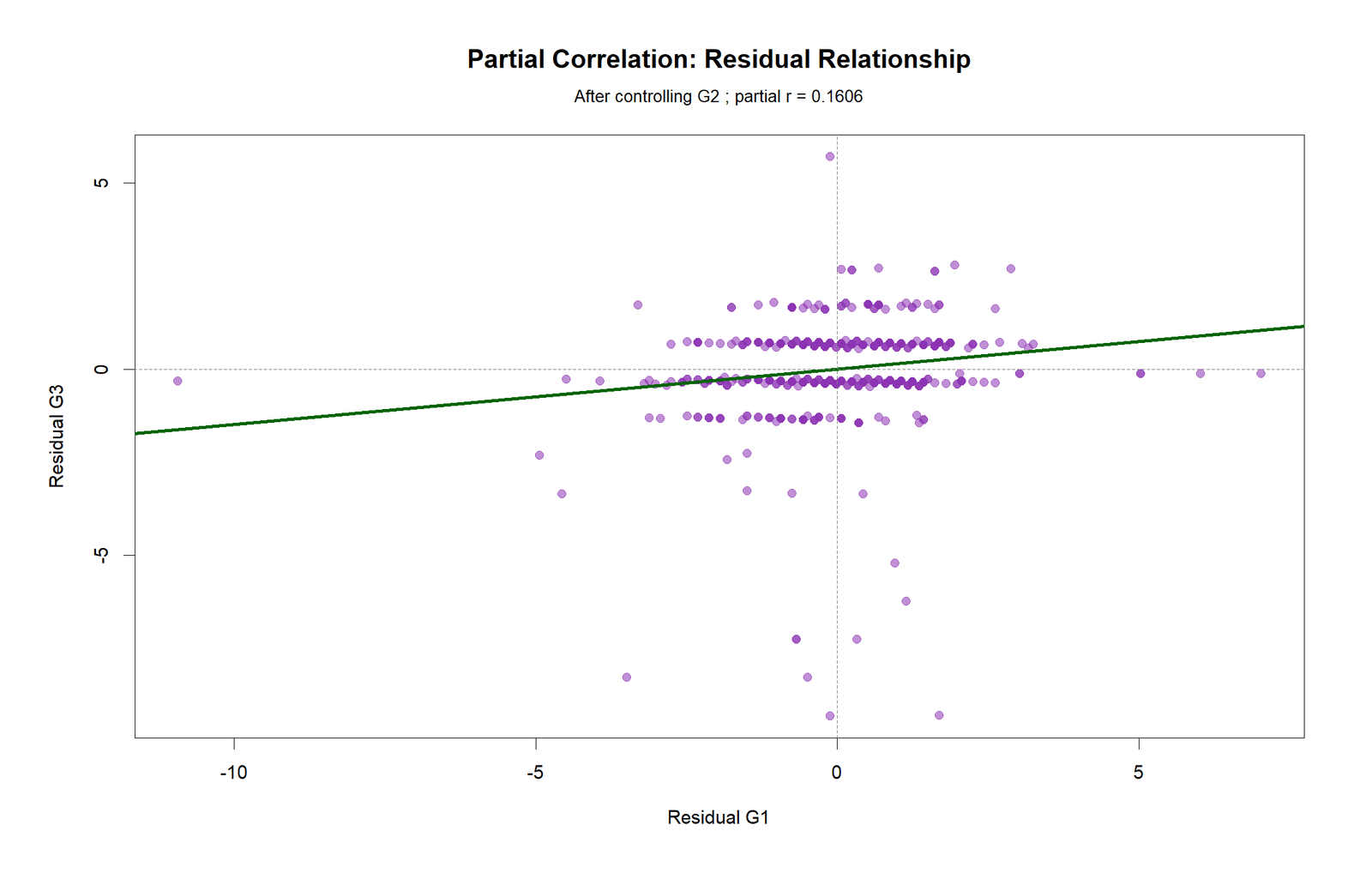
The R residual scatterplot confirms the weaker adjusted relationship. Once G2 is removed from both G1 and G3, the residual dots are much more dispersed. The remaining positive slope is small, matching the partial correlation of 0.1606.
This chart is the visual proof for the main interpretation. G1 still matters after G2 is controlled, but it no longer dominates the final grade relationship.
R Chart 3: Colorful Zero-Order vs Partial Correlation
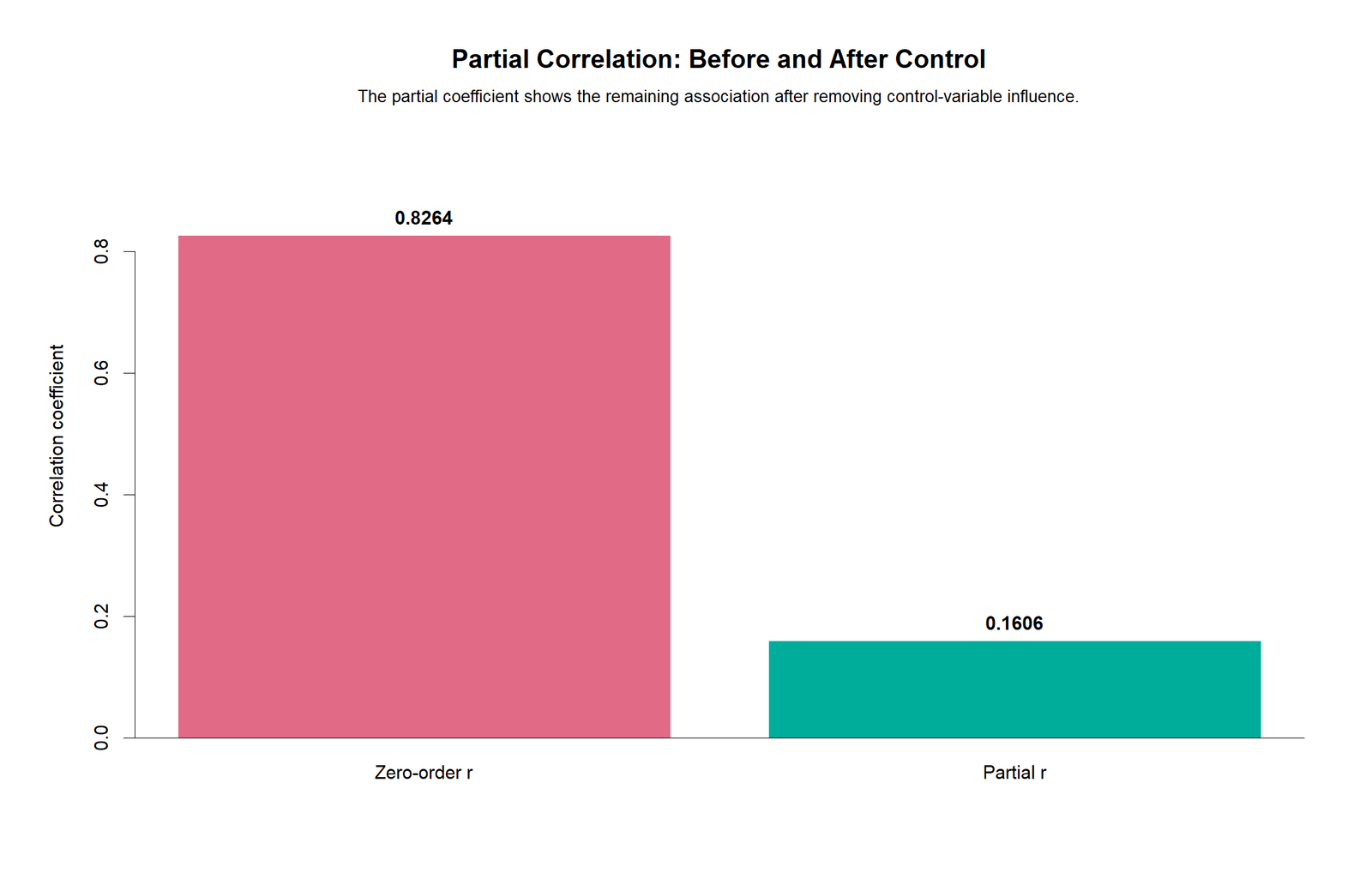
The R comparison chart repeats the same coefficient drop from 0.8264 to 0.1606. This is the most direct chart for explaining why partial correlation changes the conclusion.
The chart should be described as a reduction in the unique relationship, not as a contradiction. The raw relationship includes shared G2 information; the partial relationship removes that shared component.
R Chart 4: Colorful Partial Correlation Heatmap
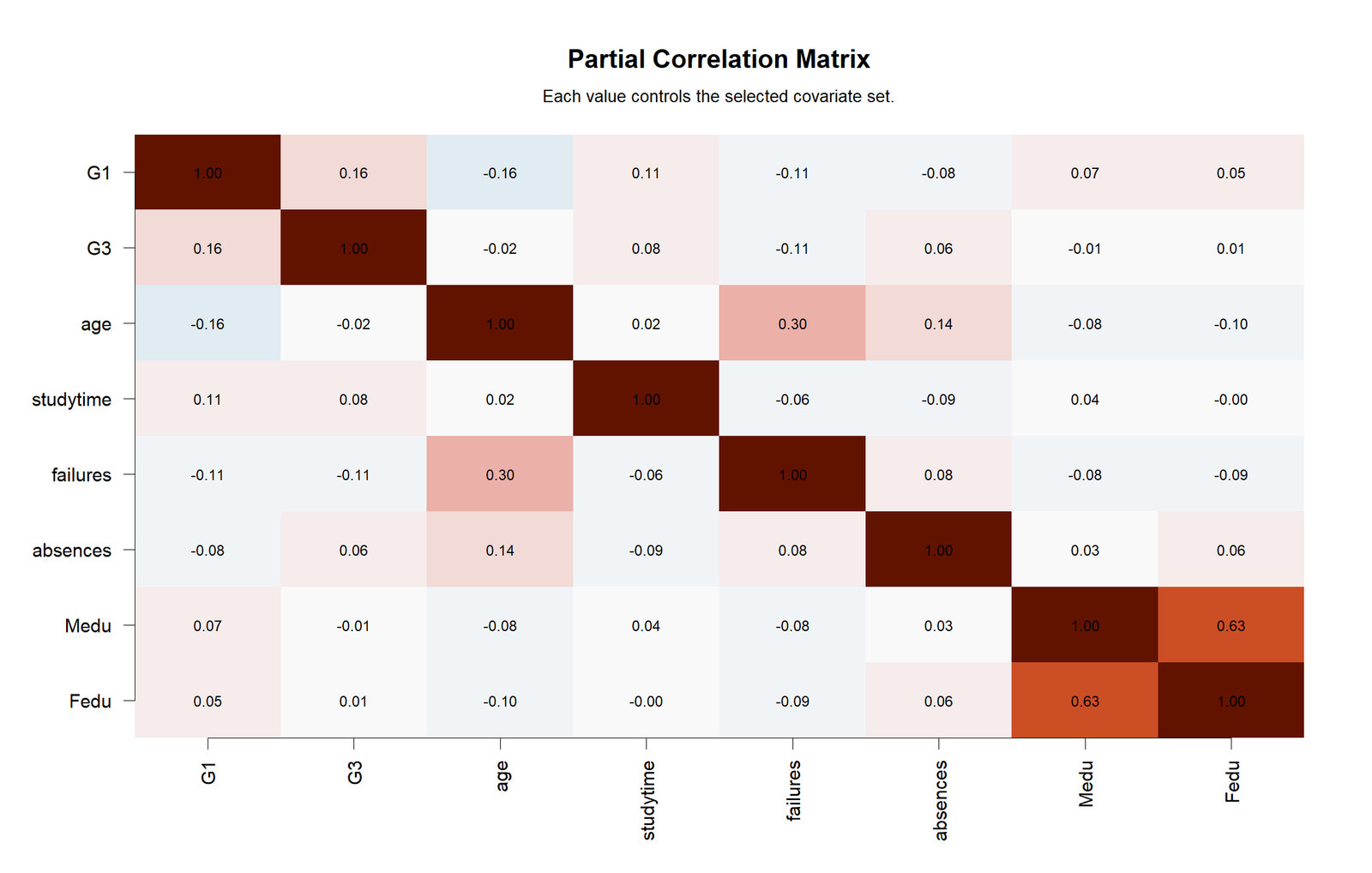
The R heatmap validates the Python heatmap. The G1-G3 adjusted cell remains positive and small, while Medu-Fedu remains one of the strongest adjusted relationships. This reinforces that partial correlation is pair-specific and context-specific.
Use this chart when readers need the broader matrix rather than only the main G1-G3 result. It shows that controlling G2 affects grade-related relationships especially strongly.
R Chart 5: Colorful Largest Pairwise Partial Correlations
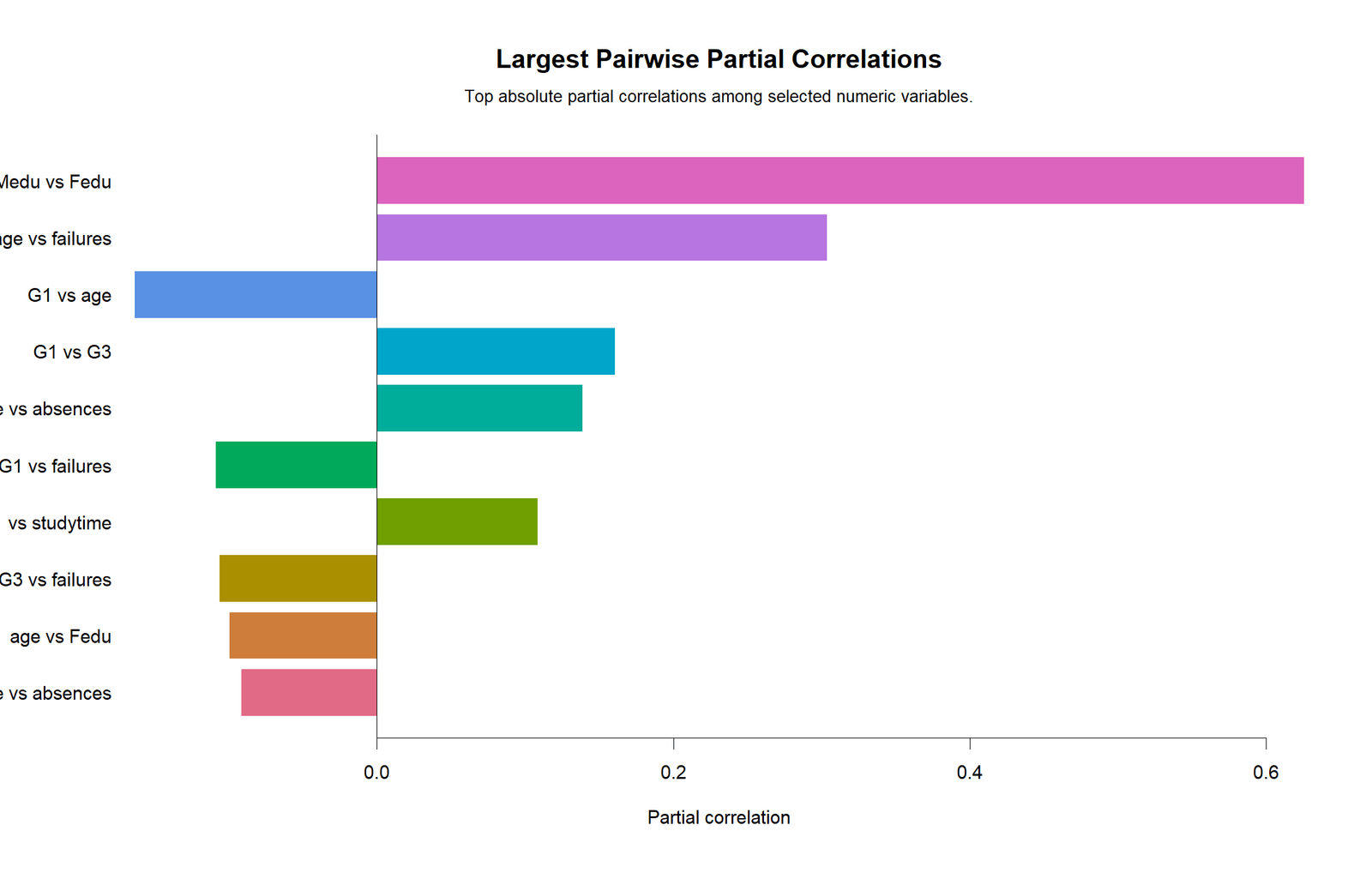
The R ranking chart confirms which adjusted pairs remain strongest. Medu and Fedu stand out, followed by other moderate or small adjusted relationships. The main G1-G3 partial correlation is present but not large.
This chart helps prevent overstatement. Statistical significance is not the same as dominance. In the controlled matrix, the adjusted G1-G3 link is meaningful but small.
R Chart 6: Colorful Partial Correlation P-Values
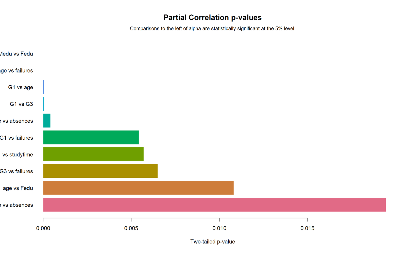
The R p-value chart confirms that the main partial correlation is statistically significant. It also shows that not every adjusted coefficient reaches significance, which is why both coefficient size and p-value must be reported together.
The final R interpretation is the same as the Python interpretation: the G1-G3 relationship remains significant after controlling G2, but its adjusted magnitude is small.
Excel Results Explained
The Excel workbook gives the clearest formula-based view of the analysis. It contains setup values, descriptive statistics, the zero-order correlation matrix, the partial correlation matrix, p-values, a worked example and a dashboard. The worked example focuses on G1 and G3 controlling G2.
Excel Worked Example: G1 and G3 Controlling G2
| Excel Item | Value | Interpretation |
|---|---|---|
| X variable | G1 | First-period grade. |
| Y variable | G3 | Final grade. |
| Control variable | G2 | Second-period grade removed from both G1 and G3. |
| N | 649 | Complete paired observations used. |
| k controls | 1 | Only G2 is controlled in the main worked example. |
| Degrees of freedom | 646 | Calculated as 649 − 1 − 2. |
| r(G1,G3) | 0.8264 | Very strong raw zero-order correlation. |
| r(G1,G2) | 0.8650 | G1 is highly related to the control variable G2. |
| r(G3,G2) | 0.9185 | G3 is very highly related to the control variable G2. |
| Partial r(G1,G3.G2) | 0.1606 | Small adjusted relationship after G2 is removed. |
| t statistic | 4.1359 | Test statistic for the partial correlation. |
| p-value | 0.000040 | Statistically significant at alpha .05. |
| Decision | Significant partial relationship | Reject H0, but describe the adjusted effect as small. |
The Excel result shows exactly why partial correlation is useful. G1 and G3 look very strongly related before adjustment. But G2 is very strongly related to both of them, so it absorbs most of the shared grade-performance information. After this shared G2 component is removed, the remaining G1-G3 association is only 0.1606.
The workbook also includes a wider partial correlation matrix controlling G2. Important values include G1 with age = -0.1637, G3 with failures = -0.1068, age with failures = 0.3038, and Medu with Fedu = 0.6257. The corresponding p-value table shows that the main G1-G3 partial relationship is significant, while some other adjusted relationships are not.
Excel interpretation rule: The formula uses ordinary correlations first, then converts them into a partial correlation. That makes Excel a good teaching tool because every step can be audited cell by cell.
Excel Formula Steps Used in the Workbook
| Step | Excel Formula Pattern | Purpose |
|---|---|---|
| Calculate rxy | =CORREL(G1_range,G3_range) | Find the zero-order correlation between the two main variables. |
| Calculate rxz | =CORREL(G1_range,G2_range) | Find the relationship between X and the control variable. |
| Calculate ryz | =CORREL(G3_range,G2_range) | Find the relationship between Y and the control variable. |
| Calculate partial r | =(rxy-rxz*ryz)/SQRT((1-rxz^2)*(1-ryz^2)) | Remove the effect of the control variable from both main variables. |
| Count N | =COUNT(G1_range) | Find the number of complete observations. |
| Calculate df | =n-k-2 | Find degrees of freedom for the significance test. |
| Calculate t | =partial_r*SQRT(df/(1-partial_r^2)) | Convert the partial correlation to a test statistic. |
| Calculate p | =T.DIST.2T(ABS(t),df) | Find the two-tailed p-value. |
| Decision | =IF(p<0.05,"Significant partial relationship","Not significant") | Make the alpha .05 decision. |
SPSS, R, Python and Excel Workflows for Partial Correlation
The same analysis can be reproduced in all four tools. The workflow always requires the same logic: choose X and Y, choose the control variable, compute the raw correlation, remove the control variable and test the adjusted relationship.
| Software | Main Steps | Best Use |
|---|---|---|
| SPSS | Run descriptives, Pearson correlations and PARTIAL CORR with G2 as the control variable. Export the Viewer output as a PDF. | Formal output, classroom verification and thesis appendix reporting. |
| Python | Use pandas for data handling, numpy/scipy for correlations and tests, residualization for partial r and matplotlib for charts. | Automated chart production, reproducible reporting and flexible dashboards. |
| R | Use cor(), lm() residuals or the one-control partial formula, then validate with cor.test() on residuals. | Statistical validation and publication-quality visual checks. |
| Excel | Use CORREL, SQRT, COUNT, T.DIST.2T and formula cells to build a transparent worked example. | Step-by-step teaching and formula auditing. |
Code Blocks for Partial Correlation
SPSS Syntax for Partial Correlation
* Partial Correlation in SPSS.
* Example: G1 and G3 controlling G2.

OUTPUT CLOSE ALL.
OUTPUT NEW NAME=Partial_Correlation_Output.

GET DATA
  /TYPE=TXT
  /FILE='dataset.csv'
  /DELCASE=LINE
  /DELIMITERS=","
  /QUALIFIER='"'
  /ARRANGEMENT=DELIMITED
  /FIRSTCASE=2
  /VARIABLES=
    school A10 sex A5 age F8.0 Medu F8.0 Fedu F8.0 studytime F8.0 failures F8.0 absences F8.0 G1 F8.2 G2 F8.2 G3 F8.2.
CACHE.
EXECUTE.

DESCRIPTIVES VARIABLES=G1 G3 G2 age studytime failures absences Medu Fedu
  /STATISTICS=MEAN STDDEV VARIANCE MIN MAX.

CORRELATIONS
  /VARIABLES=G1 G3 G2 age studytime failures absences Medu Fedu
  /PRINT=TWOTAIL
  /MISSING=LISTWISE.

PARTIAL CORR
  /VARIABLES=G1 G3 BY G2
  /SIGNIFICANCE=TWOTAIL
  /MISSING=LISTWISE.

PARTIAL CORR
  /VARIABLES=G1 G3 age studytime failures absences Medu Fedu BY G2
  /SIGNIFICANCE=TWOTAIL
  /MISSING=LISTWISE.

OUTPUT SAVE OUTFILE='Partial-Correlation-SPSS-Output.spv'.
OUTPUT EXPORT
  /CONTENTS EXPORT=VISIBLE
  /PDF DOCUMENTFILE='Partial-Correlation-SPSS-Output.pdf'.
Python Code for Partial Correlation
import pandas as pd
import numpy as np
from scipy import stats

# Load data
raw = pd.read_csv("dataset.csv")
vars_needed = ["G1", "G3", "G2", "age", "studytime", "failures", "absences", "Medu", "Fedu"]
df = raw[vars_needed].apply(pd.to_numeric, errors="coerce").dropna()

# Main variables
x = df["G1"].to_numpy(dtype=float)
y = df["G3"].to_numpy(dtype=float)
z = df[["G2"]].to_numpy(dtype=float)

# Zero-order correlation
r_xy, p_xy = stats.pearsonr(x, y)

# Residualize x and y on the control variable G2
Z = np.column_stack([np.ones(len(df)), z])
bx = np.linalg.lstsq(Z, x, rcond=None)[0]
by = np.linalg.lstsq(Z, y, rcond=None)[0]
x_resid = x - Z @ bx
y_resid = y - Z @ by

# Partial correlation is correlation between residuals
r_partial, p_partial = stats.pearsonr(x_resid, y_resid)
n = len(df)
k = 1
df_error = n - k - 2
t_value = r_partial * np.sqrt(df_error / (1 - r_partial**2))
p_from_t = stats.t.sf(abs(t_value), df_error) * 2

print("N:", n)
print("Zero-order r(G1,G3):", round(r_xy, 4))
print("Partial r(G1,G3 | G2):", round(r_partial, 4))
print("t statistic:", round(t_value, 4))
print("df:", df_error)
print("p-value:", p_from_t)
R Code for Partial Correlation
# Partial Correlation in R: G1 and G3 controlling G2

df <- read.csv("dataset.csv")
vars <- c("G1", "G3", "G2", "age", "studytime", "failures", "absences", "Medu", "Fedu")
work <- na.omit(df[vars])

# Zero-order correlation
zero_order <- cor(work$G1, work$G3)

# Formula using three Pearson correlations
r_xy <- cor(work$G1, work$G3)
r_xz <- cor(work$G1, work$G2)
r_yz <- cor(work$G3, work$G2)
partial_r <- (r_xy - r_xz * r_yz) / sqrt((1 - r_xz^2) * (1 - r_yz^2))

n <- nrow(work)
k <- 1
df_error <- n - k - 2
t_value <- partial_r * sqrt(df_error / (1 - partial_r^2))
p_value <- 2 * pt(abs(t_value), df = df_error, lower.tail = FALSE)

cat("N =", n, "\n")
cat("Zero-order r(G1,G3) =", round(zero_order, 4), "\n")
cat("Partial r(G1,G3 | G2) =", round(partial_r, 4), "\n")
cat("t =", round(t_value, 4), "df =", df_error, "p =", p_value, "\n")

# Residual method validation
x_resid <- residuals(lm(G1 ~ G2, data = work))
y_resid <- residuals(lm(G3 ~ G2, data = work))
cor.test(x_resid, y_resid)
Excel Formulas for Partial Correlation
Assume:
X = G1 range
Y = G3 range
Z = G2 control range

Zero-order correlations:
=CORREL(X_range,Y_range)     // rxy
=CORREL(X_range,Z_range)     // rxz
=CORREL(Y_range,Z_range)     // ryz

Partial correlation controlling one variable:
=(rxy-rxz*ryz)/SQRT((1-rxz^2)*(1-ryz^2))

Sample size:
=COUNT(X_range)

Degrees of freedom with one control:
=n-1-2

Test statistic:
=partial_r*SQRT(df/(1-partial_r^2))

Two-tailed p-value:
=T.DIST.2T(ABS(t),df)

Decision:
=IF(p_value<0.05,"Significant partial relationship","Not significant partial relationship")
APA Reporting Wording for Partial Correlation
When reporting a Partial Correlation, mention the two main variables, the control variable, sample size, degrees of freedom, zero-order correlation, partial correlation, p-value and practical interpretation.
APA-Style Full Report
A partial correlation was computed to examine the relationship between G1 first-period grade and G3 final grade while controlling for G2 second-period grade. The zero-order correlation between G1 and G3 was strong and positive, r = .826. After controlling for G2, the relationship was reduced to a small but statistically significant positive partial correlation, r(646) = .161, t = 4.136, p < .001. This indicates that G1 retained a small unique association with G3 after the shared grade information captured by G2 was removed.
Short APA-Style Version
G1 and G3 were strongly correlated before adjustment, r = .826. After controlling for G2, the association was small but statistically significant, partial r(646) = .161, p < .001.
Excel Worked-Example Wording
In the Excel worked example, the zero-order correlation between G1 and G3 was .8264. Because G1 and G3 were both highly correlated with G2, the partial correlation controlling G2 decreased to .1606. The adjusted relationship was statistically significant, t(646) = 4.1359, p = 0.000040, but the effect should be described as small.
Common Mistakes in Partial Correlation Interpretation
| Mistake | Why It Is a Problem | Better Practice |
|---|---|---|
| Reporting only the partial correlation | Readers cannot see how much the control variable changed the association. | Report both zero-order r and partial r. |
| Ignoring the control variable | A partial coefficient has no meaning without naming what was controlled. | Always state “controlling G2” or the exact control-variable list. |
| Calling a small significant result strong | Large samples can make small coefficients significant. | Report coefficient size and practical meaning, not only p-value. |
| Assuming control proves causation | Statistical control does not prove causal ordering. | Use causal wording only with a defensible design. |
| Confusing partial and semi-partial correlation | They remove the control variable differently. | Use partial when the control is removed from both variables; use semi-partial when removed from only one. |
| Using partial correlation with nonlinear patterns only | Linear residual correlation can miss nonlinear relationships. | Check scatterplots, residual plots and assumption diagnostics. |
When to Use Partial Correlation
Use partial correlation when you want to measure the relationship between two continuous variables while holding one or more additional variables constant. It is especially useful when a third variable may explain, inflate or hide the raw relationship.
Partial correlation is useful in education when earlier grades, attendance or background factors may affect later grades. It is useful in psychology when age, baseline ability or scale scores must be controlled. It is useful in health research when age, body mass index or baseline values must be held constant. If the goal is prediction rather than adjusted association, consider regression instead.
Downloads and Resources for Partial Correlation
R Partial Correlation Report PDFIncludes R validation charts for the same adjusted-correlation workflow.
SPSS Partial Correlation Output PDFSPSS output file for descriptives, correlations and partial correlation interpretation.
Excel Fully Worked FileExcel workbook with setup, matrices, formulas, dashboard and the G1-G3 controlling G2 worked example.
FAQs About Partial Correlation
What is partial correlation in simple words?
Partial correlation measures the relationship between two variables after removing the effect of one or more control variables.
What is the difference between correlation and partial correlation?
Correlation measures the raw relationship between two variables. Partial correlation measures their relationship after a control variable has been removed from both variables.
What was the main partial correlation result in this guide?
G1 and G3 had a zero-order correlation of 0.8264. After controlling G2, the partial correlation was 0.1606, with t(646) = 4.1359 and p = 0.000040.
How do I interpret a small but significant partial correlation?
It means the adjusted relationship is statistically detectable, usually because the sample is large, but the practical effect is small. Report both the coefficient and the p-value.
How do I calculate partial correlation in Excel?
Calculate rxy, rxz and ryz with CORREL, then use the formula (rxy-rxz*ryz)/SQRT((1-rxz^2)*(1-ryz^2)).
How do I run partial correlation in SPSS?
Use the Partial Correlations procedure, place the two main variables in the variables box and put the control variable in the controlling-for box. In syntax, use the PARTIAL CORR command.
How do I calculate partial correlation in Python?
Residualize X and Y on the control variable, then compute Pearson correlation between the two residual vectors.
How do I calculate partial correlation in R?
You can use the one-control formula from three Pearson correlations, or fit two linear models, extract residuals and run cor.test() on those residuals.
Is partial correlation the same as regression?
No. Partial correlation reports an adjusted association between two variables, while regression models prediction of an outcome from one or more predictors.
Can partial correlation prove causation?
No. Partial correlation can adjust for a control variable, but it does not prove causation by itself.

