
Regression Diagnostics, Residual Outliers, Leverage and Cook’s Distance
Studentized Residual: Formula, Interpretation, SPSS, Python, R and Excel Guide
Studentized Residual is a regression diagnostic used to identify observations whose prediction errors are unusually large after adjusting for residual standard error and leverage. In practical regression reporting, Studentized Residuals help detect possible outliers, poorly fitted cases, influential observations and model-diagnostic problems. This guide explains Studentized Residual analysis with SPSS output, Python charts, R validation charts, Excel workflow, code blocks, APA wording, common mistakes, downloadable resources, related guides and FAQ schema.
Quick Answer: Studentized Residual Result
The worked regression model predicted G3 final grade from six predictors: G1, G2, studytime, failures, absences and age. The model was strong overall, with R = .922, R² = .851, adjusted R² = .849, standard error of estimate = 1.254, and F(6, 642) = 609.353, p < .001. However, the purpose of Studentized Residual analysis is not simply to confirm model fit. The main purpose is to check whether some individual cases were predicted unusually poorly.
The SPSS residual diagnostics showed that the externally studentized deleted residual values ranged from approximately -7.59071 to 4.72741. Using the common diagnostic rule |external Studentized Residual| > 3, 10 cases were flagged as strong residual outlier candidates, representing about 1.5% of the dataset. Standardized residuals above |2| flagged 18 cases, and Cook’s distance above 4/n flagged 26 cases.
Final interpretation: The regression model predicts G3 strongly, but Studentized Residual diagnostics reveal a small group of unusual cases. These cases should not be deleted automatically. They should be reviewed for data-entry errors, legitimate unusual student performance, high leverage, Cook’s distance support and sensitivity of the regression results.
Important reporting point: A large Studentized Residual is a review signal, not a deletion order. The correct workflow is to identify the case, check the original data, examine leverage and Cook’s distance, decide whether sensitivity analysis is needed, and report the decision transparently.
Table of Contents
- What Is a Studentized Residual?
- Studentized Residual Formula
- Diagnostic Null and Alternative Hypothesis
- Dataset and Regression Variables Used
- SPSS Output Interpretation
- Python Chart-by-Chart Interpretation
- R Chart-by-Chart Validation
- SPSS, R, Python and Excel Workflows
- Code Blocks for Studentized Residual
- APA Reporting Wording
- Common Mistakes
- When to Use Studentized Residuals
- Downloads and Resources
- Related Guides
- FAQs
What Is a Studentized Residual?
A Studentized Residual is a residual divided by an estimate of its standard error. A raw residual tells how far an observed value is from its predicted value. A standardized residual divides that prediction error by the overall residual standard deviation. A Studentized Residual improves the diagnostic by also considering the fact that different cases can have different leverage and therefore different residual variance.
In regression, some observations are easier for the model to predict than others. A case with an unusual predictor pattern can have high leverage. A case can also have a very unusual outcome compared with the fitted model. Studentized Residual analysis helps identify the second issue: cases where the observed outcome is far from the model prediction after proper scaling.
The most useful version for outlier screening is often the externally Studentized Residual, also called the studentized deleted residual. It is calculated by excluding the case from the residual variance estimate. This makes it more sensitive for identifying observations that may be unusually inconsistent with the rest of the regression model.
Simple definition: A Studentized Residual is like a z score for a regression prediction error. Values near 0 mean the case is predicted well. Values beyond ±2 deserve attention. Values beyond ±3 are commonly flagged as strong residual outlier candidates.
Studentized Residual analysis belongs inside a broader regression diagnostic workflow. It should be interpreted together with residual plots, leverage, Cook’s distance, DFFITS, normality checks, homoscedasticity checks and model specification checks. Useful related guides include the Ramsey RESET test, Goldfeld-Quandt test, Q-Q plot normality check, and P-P plot normality check.
Studentized Residual Formula
The raw residual for case i is the difference between the observed outcome and the predicted outcome:
The internally Studentized Residual divides the raw residual by the residual standard error adjusted for leverage:
The externally Studentized Residual, also called the studentized deleted residual, uses the residual standard error calculated without case i:
| Symbol | Meaning | Interpretation |
|---|---|---|
| ei | Raw residual | Observed value minus predicted value. |
| yi | Observed outcome | The actual value of G3 for case i. |
| ŷi | Predicted outcome | The fitted G3 value from the regression model. |
| s | Residual standard error | Model-level estimate of residual spread. |
| s(i) | Deleted residual standard error | Residual spread after excluding case i. |
| hii | Leverage | Shows how unusual the predictor profile is. |
| ri | Internally Studentized Residual | Residual scaled using the full-model error estimate. |
| ti | Externally Studentized Residual | Residual scaled using deleted-case error estimate. |
Threshold rule: A common diagnostic rule is to review cases where |Studentized Residual| > 2 and strongly flag cases where |Studentized Residual| > 3. These thresholds are diagnostic signals, not automatic deletion rules.
Diagnostic Null and Alternative Hypothesis for Studentized Residual
A Studentized Residual is not usually reported as a single traditional p-value test. It is interpreted through diagnostic thresholds. However, a hypothesis-style statement helps readers understand the decision rule.
| Statement | Diagnostic Rule | Meaning |
|---|---|---|
| Null diagnostic assumption | H0: No case has |external Studentized Residual| > 3 | No strong residual outlier candidate is detected. |
| Alternative diagnostic assumption | H1: At least one case has |external Studentized Residual| > 3 | At least one case is a strong residual outlier candidate. |
| Influence support rule | Cook’s distance > 4/n | The case may have practical influence on the fitted model. |
Decision for this example: The diagnostic null assumption is not supported because 10 cases had |external Studentized Residual| > 3. This means the model contains a small number of strong residual outlier candidates. These cases should be reviewed, especially when a large Studentized Residual also appears with meaningful Cook’s distance.
Dataset and Regression Variables Used
The worked example uses a student performance regression model. The dependent variable is G3 final grade. The predictors are G1, G2, studytime, failures, absences and age. The sample contains 649 valid cases. The model is useful for a Studentized Residual lesson because it predicts G3 strongly while still containing a small set of cases with unusual prediction errors.
| Variable | Role | Why It Matters for Studentized Residual Analysis |
|---|---|---|
| G3 | Dependent variable | The observed outcome being predicted. Studentized Residuals measure unusual prediction errors for G3. |
| G1 | Predictor | First-period grade. Strong predictor of final grade and related to G2. |
| G2 | Predictor | Second-period grade. Strongest predictor in the model and central to fitted values. |
| studytime | Predictor | Study-time category. Included as a learning behavior predictor. |
| failures | Predictor | Previous class failures. Negative predictor and useful context for unusual performance. |
| absences | Predictor | Absence count. Helps explain grade variation and can support outlier interpretation. |
| age | Predictor | Student age. Included to adjust for demographic variation. |
Before interpreting Studentized Residuals, it is useful to understand the distribution of the variables using descriptive statistics, frequency distributions, histograms, box plots, and the five-number summary.
SPSS Output Interpretation for Studentized Residual
The SPSS output provides the main verification for the Studentized Residual example. SPSS fitted the regression model, saved residual diagnostics, produced residual descriptive statistics, tested residual normality, counted diagnostic flags, listed the largest absolute studentized deleted residuals and summarized the case-level review problem.
SPSS Regression Model Summary
| SPSS Output Item | Value | Interpretation |
|---|---|---|
| Dependent variable | G3 | The regression predicts final grade. |
| Predictors | age, studytime, absences, G2, failures, G1 | All requested predictors were entered together. |
| R | .922 | The fitted values are strongly related to observed G3 values. |
| R Square | .851 | About 85.1% of the variance in G3 is explained by the predictors. |
| Adjusted R Square | .849 | The model remains strong after adjusting for six predictors. |
| Standard error of estimate | 1.254 | Typical prediction error is about 1.254 grade points. |
| ANOVA | F(6, 642) = 609.353, p < .001 | The overall regression model is statistically significant. |
SPSS Coefficients and Predictor Context
| Predictor | B | Beta | t | p | Tolerance | VIF | Interpretation |
|---|---|---|---|---|---|---|---|
| G1 | .142 | .121 | 3.886 | < .001 | .241 | 4.155 | Significant positive predictor; related to G2 but VIF remains below 5. |
| G2 | .883 | .797 | 25.823 | < .001 | .244 | 4.091 | Strongest positive predictor of G3. |
| studytime | .095 | .024 | 1.526 | .127 | .919 | 1.088 | Not statistically significant after other predictors are controlled. |
| failures | -.233 | -.043 | -2.456 | .014 | .766 | 1.306 | Significant negative predictor. |
| absences | .023 | .033 | 2.086 | .037 | .954 | 1.049 | Small but statistically significant positive coefficient in the adjusted model. |
| age | .024 | .009 | .544 | .587 | .866 | 1.155 | Not statistically significant after other predictors are controlled. |
SPSS Residual Statistics
| Diagnostic Statistic | Minimum | Maximum | Mean | Std. Deviation | Meaning |
|---|---|---|---|---|---|
| Raw residual | -9.04462 | 5.81680 | .00000 | 1.24859 | Prediction error in original G3 grade units. |
| Standardized residual | -7.27663 | 4.65072 | -.00036 | 1.00177 | Residual scaled by model residual error. |
| Studentized deleted residual | -7.59071 | 4.72741 | -.00271 | 1.01878 | Externally Studentized Residual used for strong outlier review. |
| Leverage | .00064 | .10177 | .00925 | .01002 | Unusual predictor pattern indicator. |
| Cook’s distance | .00000 | .17695 | .00186 | .00985 | Influence indicator combining residual size and leverage. |
| DFFITS | -.21108 | .12933 | -.00090 | .02028 | Case influence on its fitted value. |
SPSS Diagnostic Flag Counts
| Diagnostic Rule | Flagged Cases | Percent | Interpretation |
|---|---|---|---|
| |standardized residual| > 2 | 18 | 2.8% | Moderate residual outlier warning group. |
| |studentized deleted residual| > 3 | 10 | 1.5% | Strong residual outlier candidate group. |
| Cook’s distance > 4/n | 26 | 4.0% | Cases with possible influence support. |
Largest Absolute Studentized Deleted Residuals
| Case | Observed G3 | Predicted G3 | Raw Residual | External Studentized Residual | Cook’s Distance | Interpretation |
|---|---|---|---|---|---|---|
| 164 | 0 | 9.02294 | -9.02294 | -7.59071 | .17695 | Most extreme negative residual and highest Cook’s distance. |
| 173 | 1 | 10.04462 | -9.04462 | -7.54523 | .05473 | Very large negative residual; strong review candidate. |
| 587 | 0 | 8.25028 | -8.25028 | -6.83144 | .04489 | Large negative residual; model strongly overpredicted G3. |
| 640 | 0 | 7.54332 | -7.54332 | -6.25288 | .10887 | Large negative residual with meaningful influence support. |
| 520 | 0 | 7.34324 | -7.34324 | -6.04006 | .04366 | Large negative residual; review student context. |
| 638 | 0 | 7.15378 | -7.15378 | -5.88893 | .06191 | Strong negative residual outlier candidate. |
| 641 | 0 | 6.92062 | -6.92062 | -5.67882 | .04539 | Strong negative residual outlier candidate. |
| 584 | 0 | 6.17939 | -6.17939 | -5.05284 | .04700 | Large negative residual; model overpredicted final grade. |
| 62 | 16 | 10.18320 | 5.81680 | 4.72741 | .01820 | Strong positive residual; model underpredicted final grade. |
| 627 | 0 | 5.48156 | -5.48156 | -4.47339 | .04947 | Large negative residual; review as outlier candidate. |
SPSS Normality and Residual Shape
SPSS residual normality checks showed that the studentized deleted residual distribution was not perfectly normal. This is expected when the distribution contains a small number of extreme residuals. The issue does not automatically invalidate the regression model, especially with a large sample, but it does support visual inspection through histograms, Q-Q plots, P-P plots and case-level residual charts.
SPSS interpretation summary: The model fit is strong, but Studentized Residual diagnostics identify a small set of unusual cases. Ten cases exceed the |external Studentized Residual| > 3 rule. The largest concern is case 164, which combines an extreme negative residual with the highest Cook’s distance. These cases should be reviewed before final reporting, but they should not be removed without substantive justification.
Python Chart-by-Chart Interpretation
The Python charts below show the complete Studentized Residual diagnostic workflow. They include residuals versus fitted values, case-index residuals, residual distribution, leverage comparison, top residual cases, diagnostic flag counts and Cook’s distance support.
Python Chart 1: Studentized Residuals vs Fitted Values
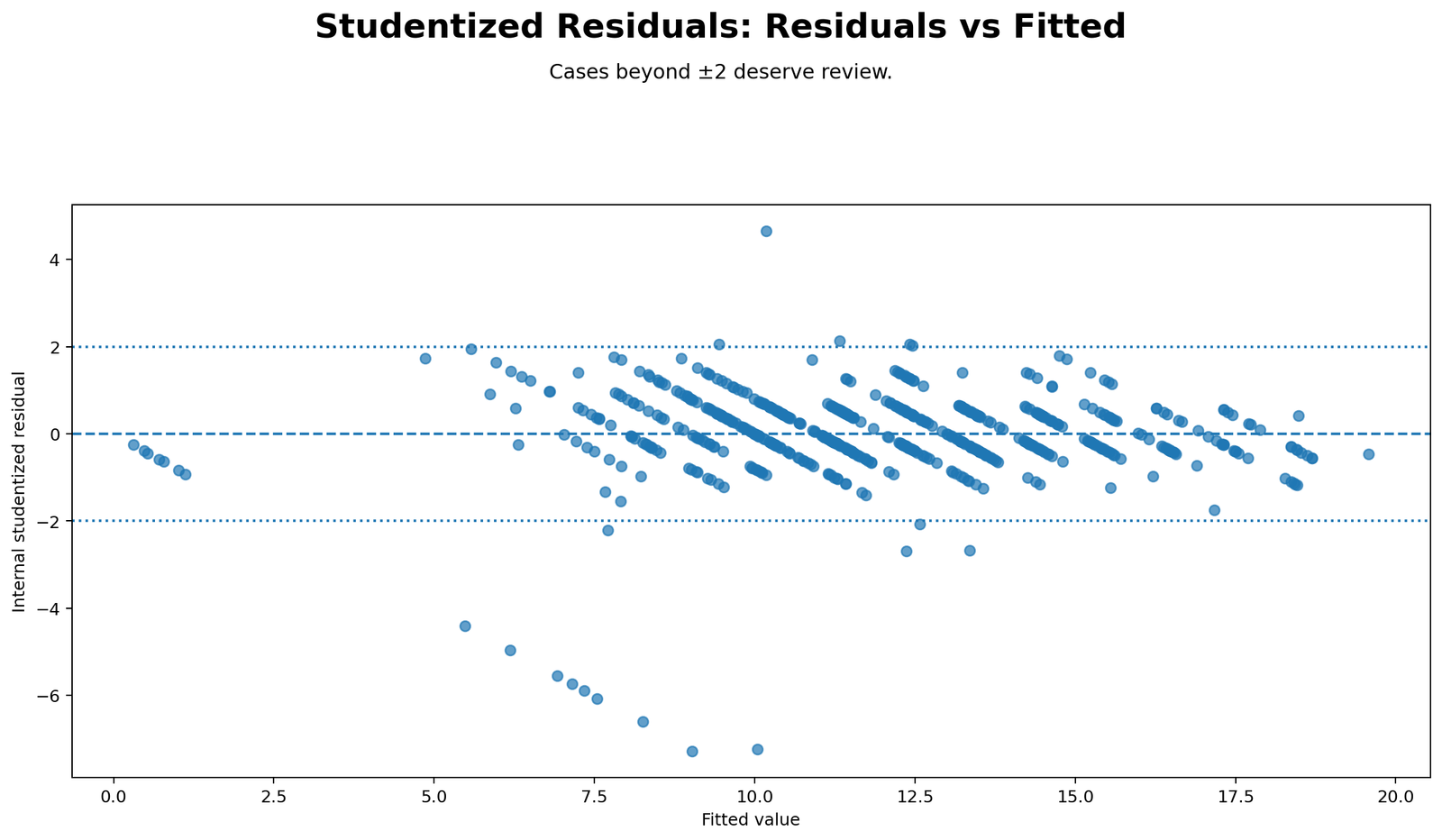
This chart compares Studentized Residuals with fitted G3 values. A good residual plot should mostly show points scattered around zero without strong curves, funnels or systematic clusters. In this example, most cases sit near the center, but several points fall far below the usual ±2 and ±3 review zones. These negative residuals show cases where the model predicted a higher G3 score than the student actually received.
The chart is important because a single residual table does not show where unusual cases occur across the fitted range. If extreme residuals appear only in one fitted-value region, it may suggest model misspecification, nonlinear relationships, subgroup problems or missing predictors. The Python plot supports the SPSS conclusion that the model is generally strong but has a small set of unusual prediction errors.
Python Chart 2: External Studentized Residual Index
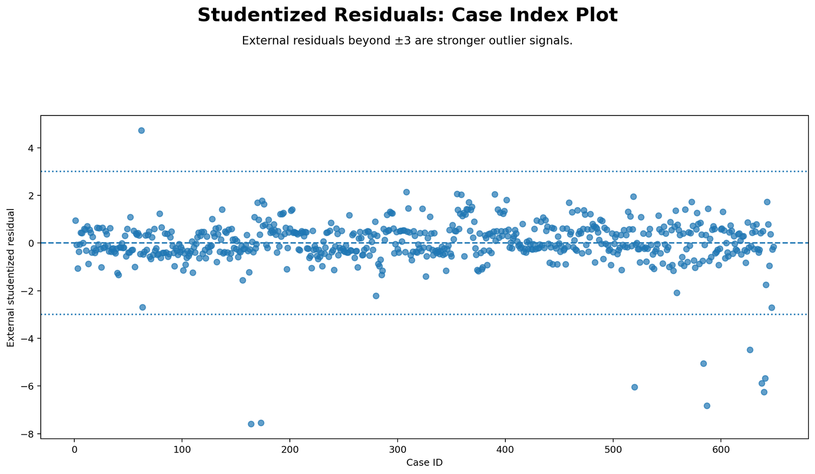
The index chart makes it easier to locate case-level spikes. The strongest negative residuals appear as sharp downward points, while one strong positive residual appears above the upper threshold. This matches the SPSS list of largest absolute studentized deleted residuals, where case 164, case 173, case 587, case 640, case 520, case 638, case 641, case 584, case 62 and case 627 were among the most important review cases.
This chart is especially useful for audit work. A researcher can connect the case index to the original record, check whether the values are valid, and decide whether the residual is caused by data entry, real unusual behavior, a subgroup effect or a missing explanatory variable.
Python Chart 3: Studentized Residual Distribution
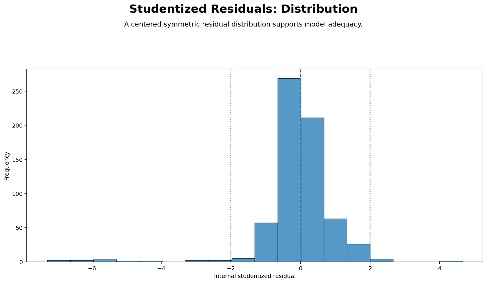
The distribution chart shows that most Studentized Residuals are near zero, which is expected in a fitted regression model. However, the distribution has clear tail behavior caused by extreme residual cases. The negative tail is especially important because several students had much lower G3 scores than the model predicted from G1, G2 and other predictors.
This chart supports the SPSS residual statistics. The residual distribution is centered near zero, but it is not perfectly normal because of extreme cases. In a large sample, the model may still be useful, but the diagnostic report should mention the unusual residual cases.
Python Chart 4: Leverage vs Absolute Studentized Residual
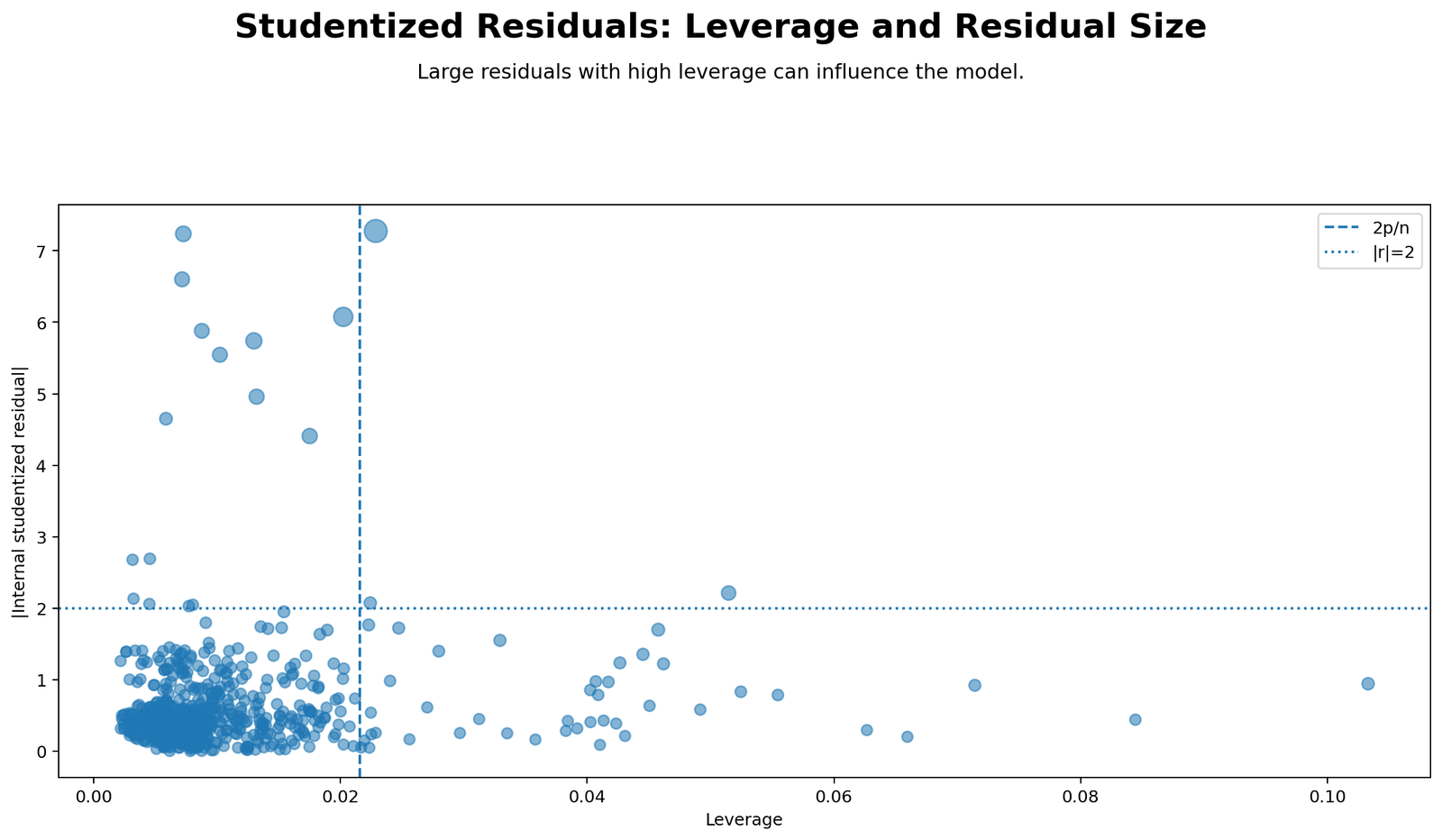
This chart combines two diagnostic ideas. Studentized Residuals show outcome unusualness, while leverage shows predictor-profile unusualness. A case with a high absolute Studentized Residual but low leverage is mainly an outcome outlier. A case with high leverage but a small residual may affect the fitted model shape but not appear as a large prediction error. A case with both high leverage and high absolute residual is a stronger diagnostic concern.
The plot helps distinguish “unusual outcome” from “influential case.” This matters because not every residual outlier changes the regression model strongly. Cook’s distance is then used as support to decide whether the unusual residual also has influence.
Python Chart 5: Top External Studentized Residuals
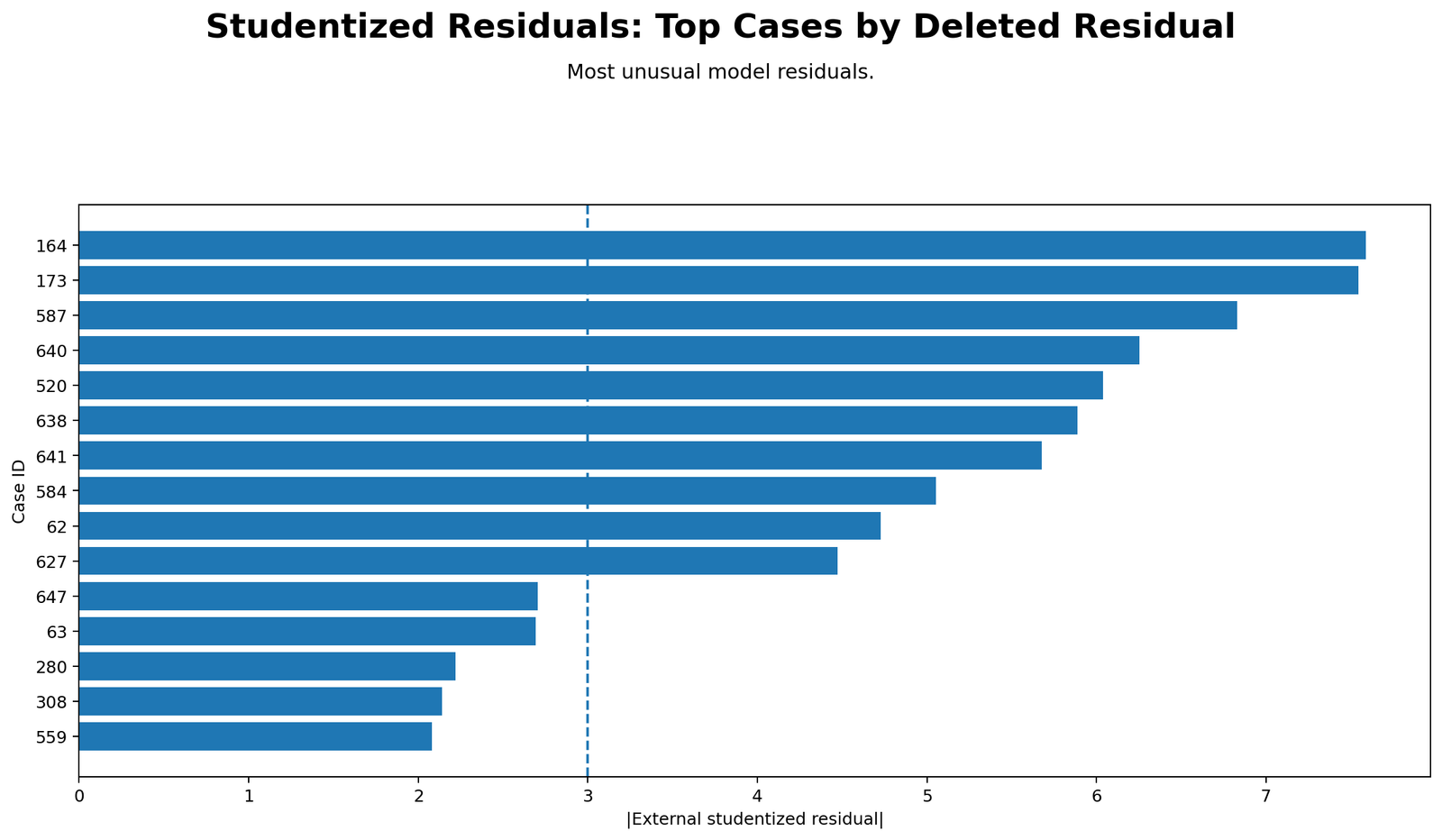
This chart ranks the strongest residual outlier candidates. The largest negative cases are students whose final G3 grade was much lower than the model predicted. The strongest positive case is a student whose G3 grade was much higher than predicted. The most extreme case in the SPSS list is case 164, with an external Studentized Residual near -7.59.
The chart is useful for reporting because it gives a readable case-level summary. Instead of saying only “10 cases exceeded |3|,” the chart shows which cases were most important and in which direction the model failed to predict accurately.
Python Chart 6: Diagnostic Flag Counts
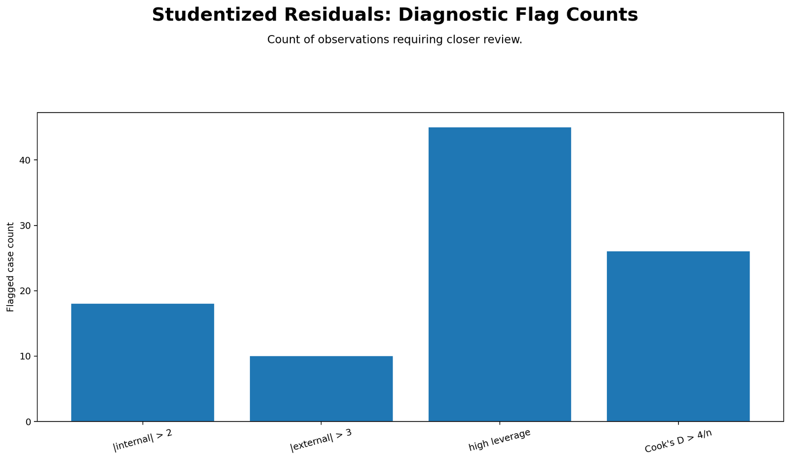
The diagnostic flag count chart summarizes the main decision rules. The SPSS output showed 18 cases above |standardized residual| > 2, 10 cases above |external Studentized Residual| > 3, and 26 cases above Cook’s distance > 4/n. These counts show that the dataset contains a small but important group of cases requiring review.
The chart also shows why multiple diagnostics are needed. Cook’s distance flagged more cases than external Studentized Residuals. This means some cases may be influential because of leverage and residual combination even if they are not among the most extreme residual outliers.
Python Chart 7: Cook’s Distance Support
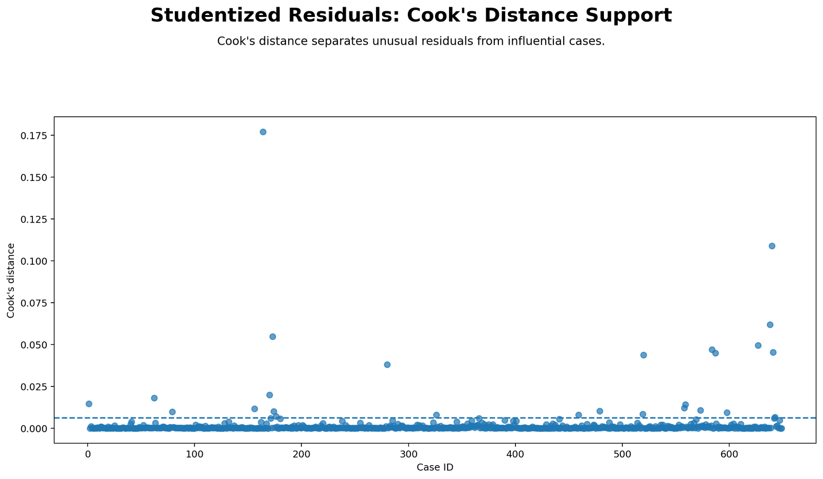
This chart links Studentized Residual size with influence. A large residual alone means the model predicted poorly for a case. A large Cook’s distance means the case may also affect the fitted regression coefficients or predicted values. The most important review cases are those that combine large absolute Studentized Residuals with nontrivial Cook’s distance.
In the SPSS output, case 164 had both the most extreme external Studentized Residual and the highest Cook’s distance. This makes it a priority case for review. However, even this does not mean automatic deletion. The correct approach is to inspect the original record, understand why it is unusual, run sensitivity analysis if needed, and report the decision transparently.
R Chart-by-Chart Validation
The R charts validate the Python and SPSS conclusions using a separate workflow. The R visual pattern is the same: the model fits G3 strongly, most residuals are close to zero, and a small group of cases has large external Studentized Residuals. This software-to-software agreement strengthens confidence in the diagnostic interpretation.
R Chart 1: Studentized Residuals vs Fitted Values
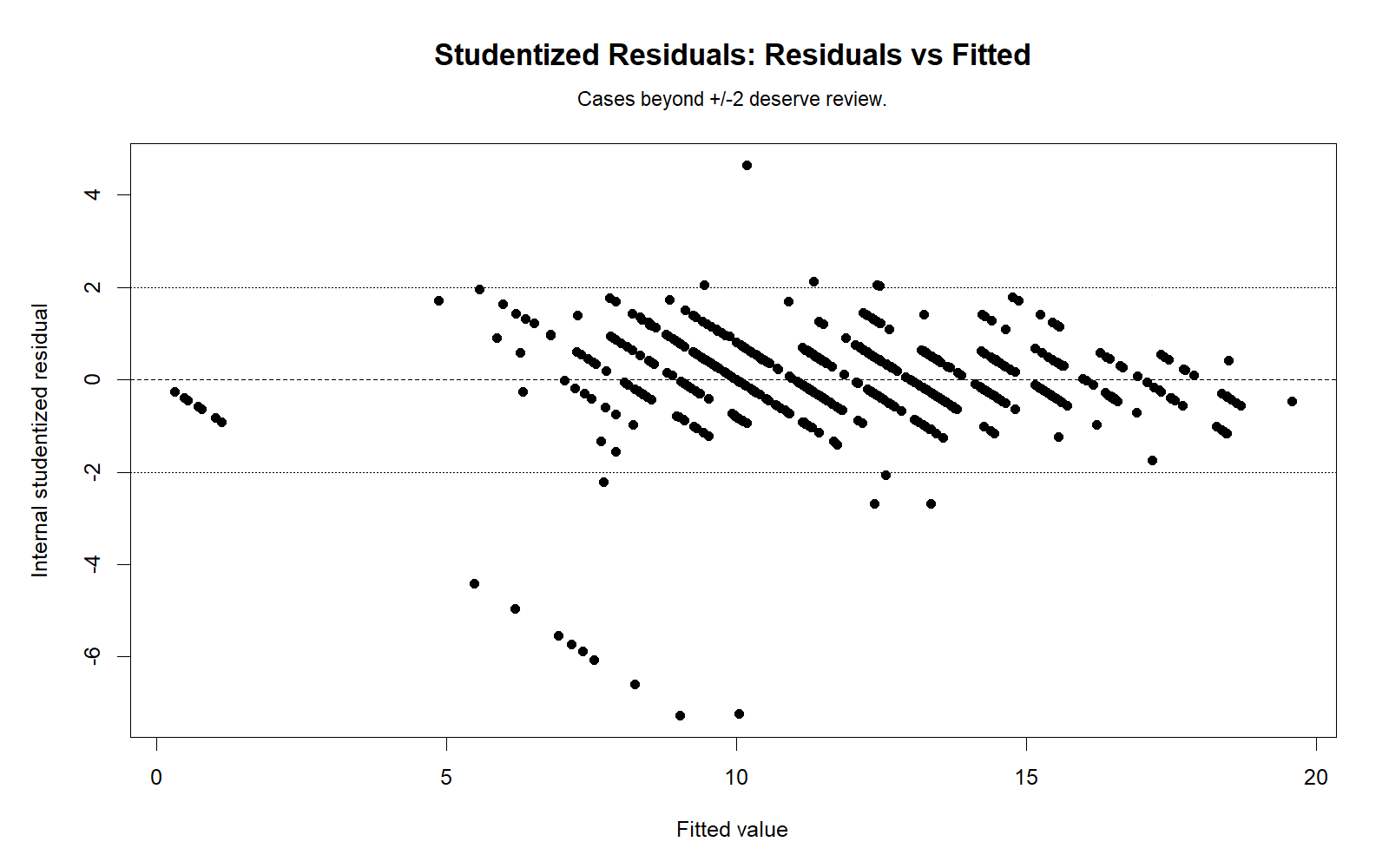
The R residuals-versus-fitted chart confirms the Python pattern. Most cases cluster around the zero residual line, but a small number of cases sit far from the expected range. The extreme negative cases show that the model predicted higher G3 values than the observed values for those students.
The R chart validates that the residual pattern is not a software artifact. It is a real diagnostic feature of the regression model and should be discussed in the residual diagnostics section of the report.
R Chart 2: External Studentized Residual Index
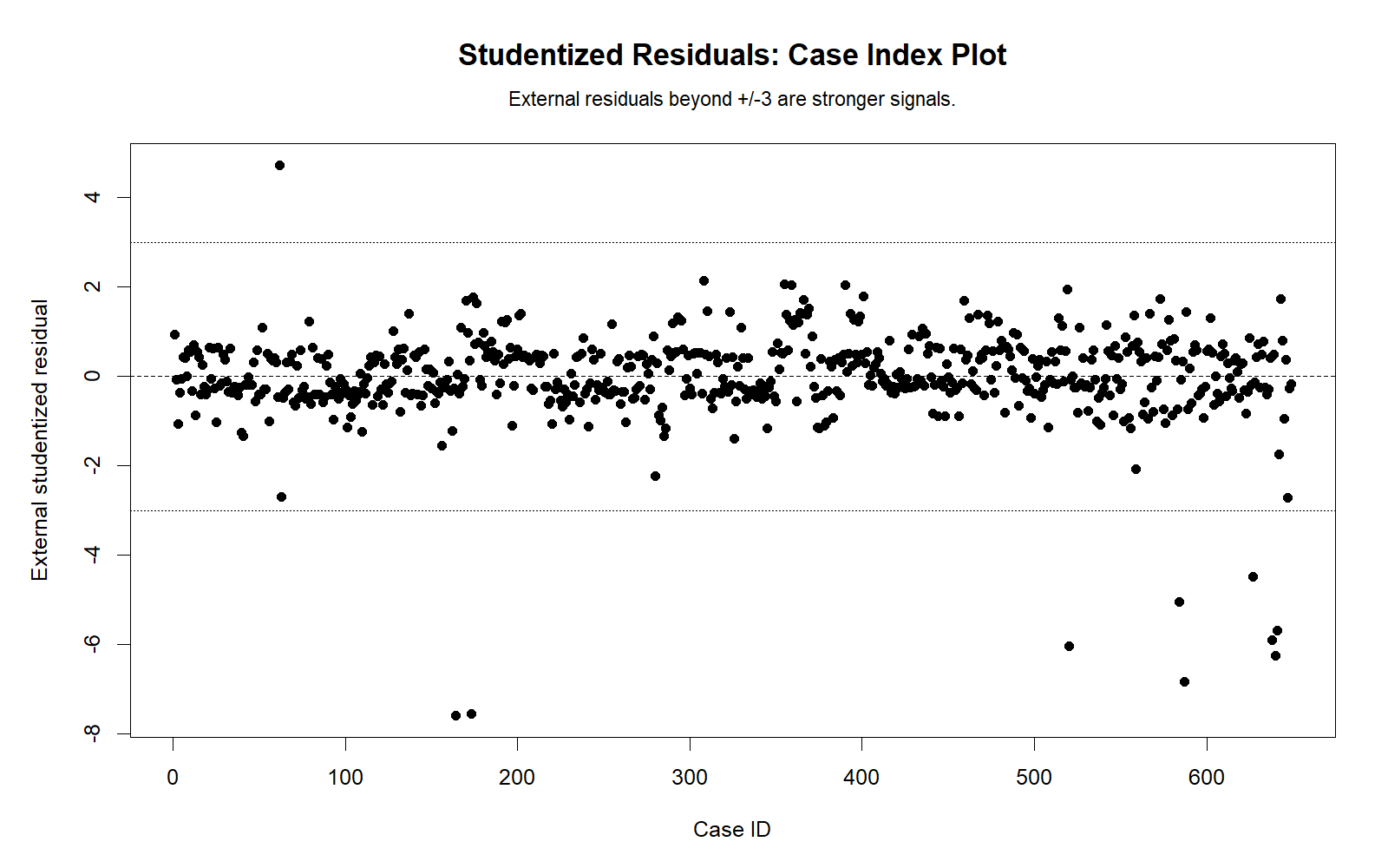
The R index chart confirms the case-level residual spikes. The same strong negative residual group appears, and the same diagnostic logic applies: cases beyond the ±3 threshold should be reviewed as strong residual outlier candidates.
Case-index charts are useful because they allow the analyst to trace back from the plotted diagnostic point to the original row in the dataset. That is essential for transparent outlier review.
R Chart 3: Studentized Residual Distribution
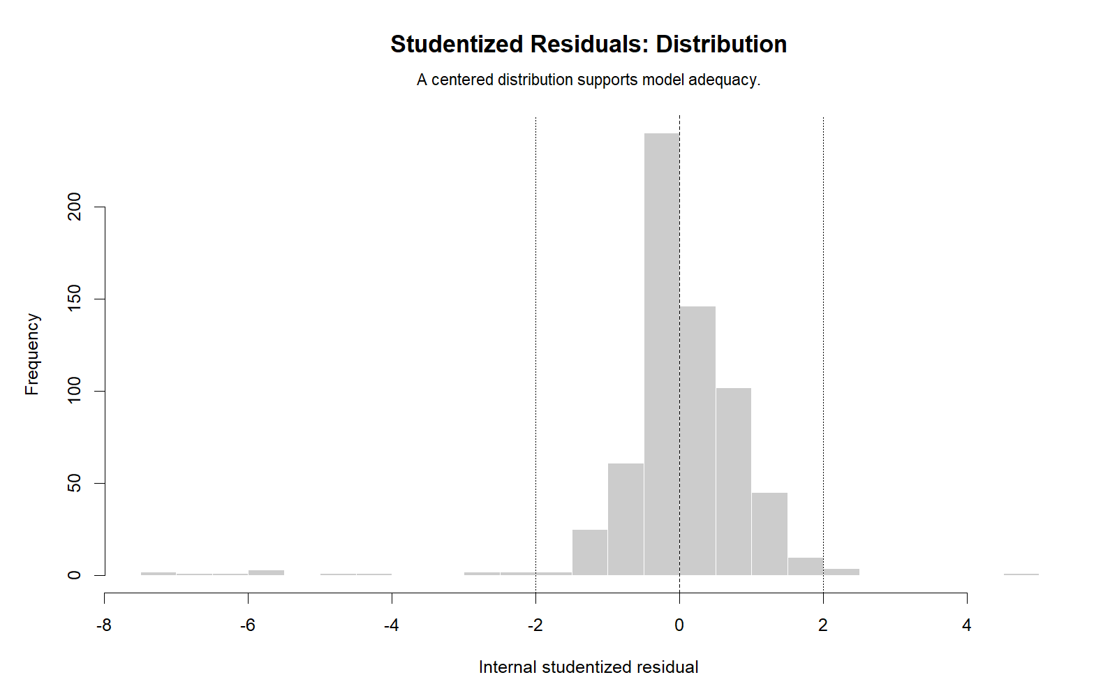
The R distribution chart confirms that the Studentized Residuals are centered near zero but contain long-tail cases. This supports the SPSS descriptive statistics, where the studentized deleted residual mean was close to zero and the standard deviation was close to one, but the minimum and maximum values were extreme.
The chart supports a balanced conclusion: the model is useful overall, but a few cases create tail behavior that should be reviewed and disclosed.
R Chart 4: Leverage vs Absolute Studentized Residual
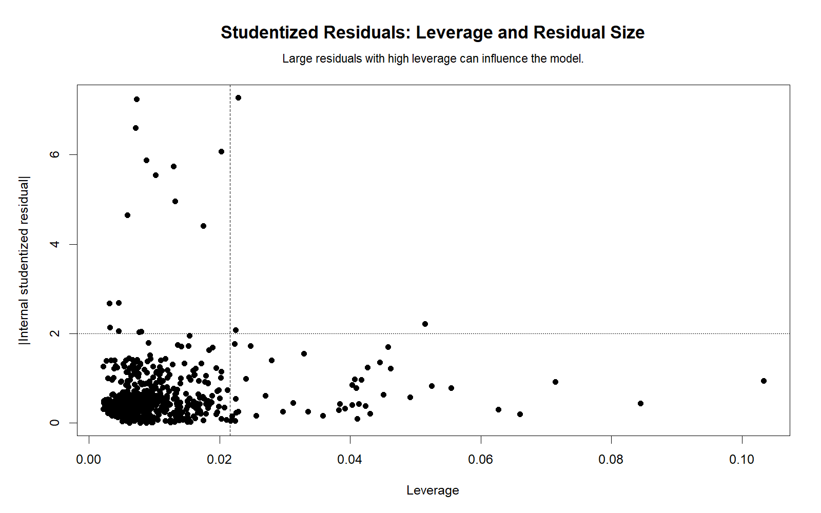
The R leverage chart confirms that residual size and leverage are different diagnostic dimensions. A case can have a large residual without high leverage, or high leverage without a large residual. The strongest follow-up cases are those that are unusual in both outcome and predictor pattern.
This chart should be interpreted with Cook’s distance because influence is a combination of residual size and leverage. A large residual is important, but influence depends on whether the case meaningfully changes the fitted model.
R Chart 5: Top External Studentized Residuals
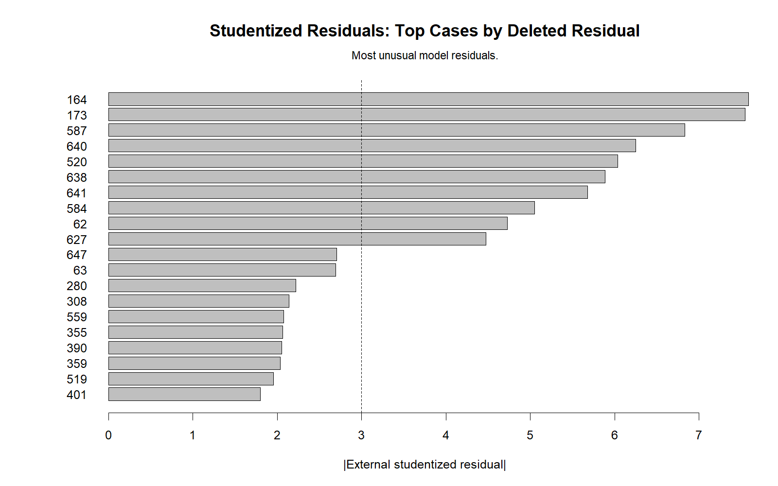
The R top-case chart validates the same review list. It confirms that the outlier concern is not caused by one software package. The largest negative residuals correspond to students whose final grades were much lower than the model predicted.
The visual ranking is helpful for final reporting because it turns a long residual output table into a clear diagnostic summary. The analyst can identify the most important cases and discuss the review process.
R Chart 6: Diagnostic Flag Counts
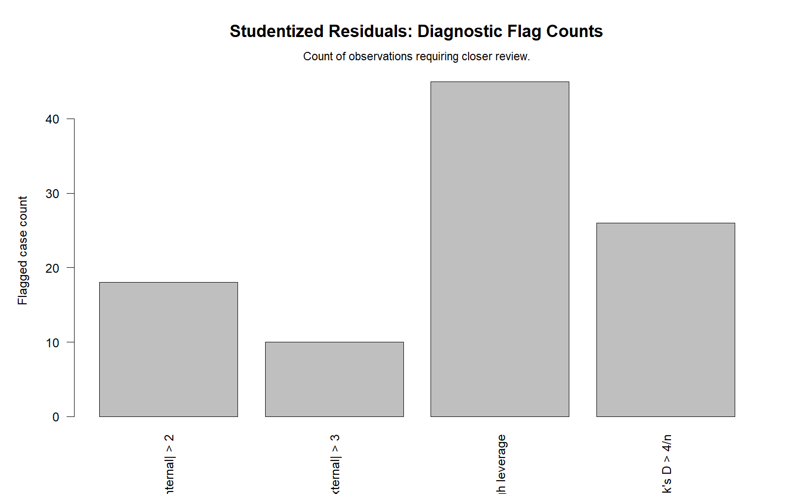
The R flag-count chart validates the same diagnostic summary as SPSS and Python. A small percentage of cases were flagged by residual and influence rules. This is common in many real datasets, but it must be disclosed when reporting regression diagnostics.
Flag counts are also useful because they prevent overreacting to a single case. The report can say how many cases exceeded each rule, then discuss whether those cases materially affected the analysis.
R Chart 7: Cook’s Distance Support
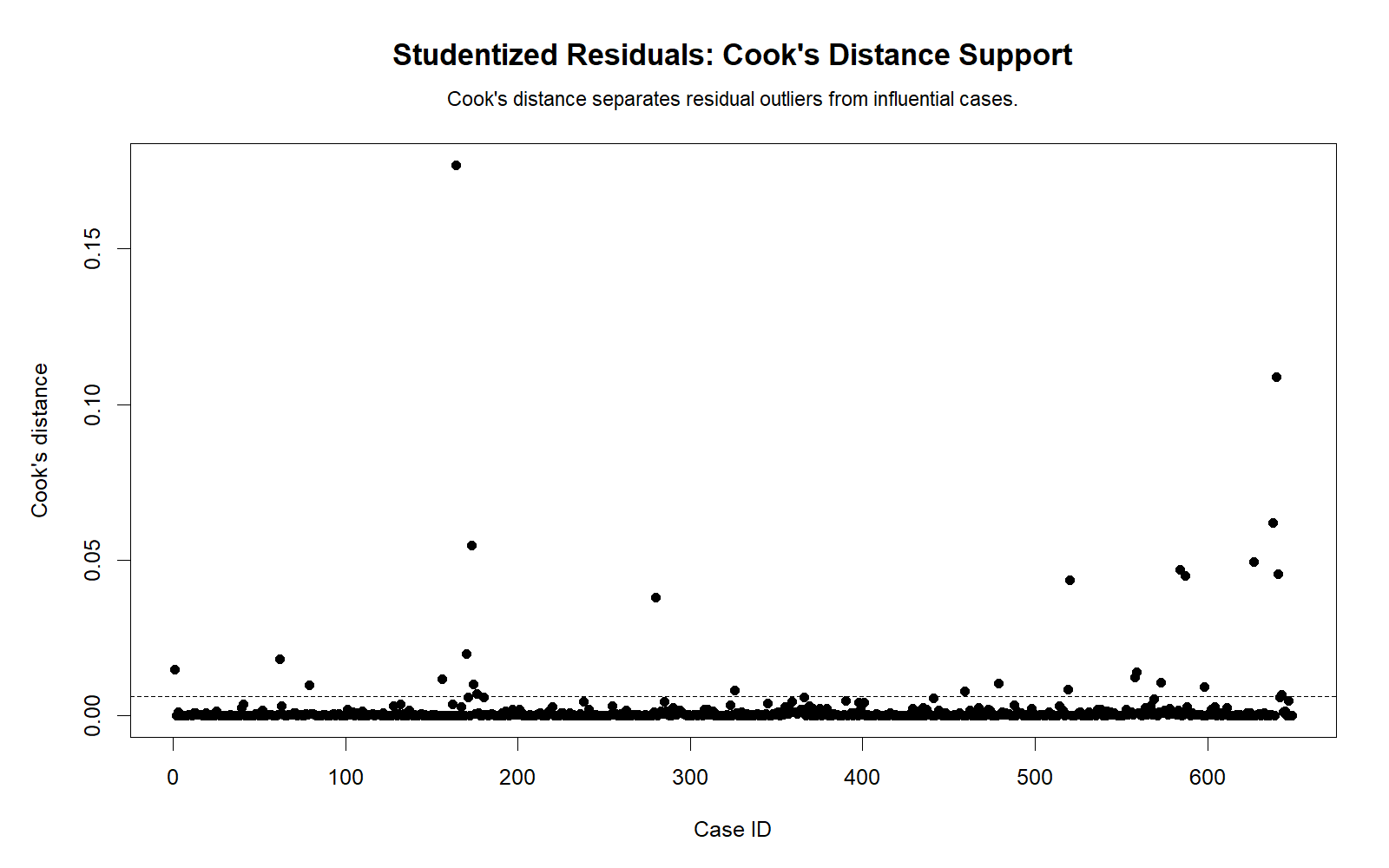
The R Cook’s distance chart confirms that not all residual outliers are equally influential. Cases with high residuals and meaningful Cook’s distance are the most important for sensitivity review. This chart supports the conclusion that the residual diagnostics require case review, not automatic model rejection.
The final R validation message matches Python and SPSS: the model performs strongly overall, but the Studentized Residual diagnostics identify a small set of cases that should be checked carefully.
SPSS, R, Python and Excel Workflows for Studentized Residual
The same Studentized Residual workflow can be reproduced in SPSS, R, Python and Excel. SPSS can save studentized deleted residuals directly. R and Python can calculate externally Studentized Residuals through model influence functions. Excel can calculate a simplified residual diagnostic workflow by computing residuals, leverage, standard errors and internally Studentized Residuals manually.
SPSS Workflow
| Step | SPSS Menu or Syntax | Purpose |
|---|---|---|
| Open dataset | File > Open > Data | Load the clean dataset. |
| Run regression | Analyze > Regression > Linear | Set G3 as dependent variable and enter G1, G2, studytime, failures, absences and age. |
| Save residual diagnostics | Save > Residuals and influence statistics | Save standardized residuals, studentized residuals, deleted residuals, leverage and Cook’s distance. |
| Review residual statistics | Regression output > Residuals Statistics | Check minimum, maximum, mean and standard deviation of residual diagnostics. |
| Flag cases | Transform > Compute Variable | Create rules such as |studentized deleted residual| > 3 and Cook’s distance > 4/n. |
| List top cases | Sort by absolute studentized deleted residual | Inspect the largest residual cases and compare with Cook’s distance. |
| Export output | File > Export or OUTPUT EXPORT | Save a PDF for reporting and verification. |
R Workflow
| Step | R Action | Purpose |
|---|---|---|
| Read data | read.csv() | Load the dataset. |
| Fit regression model | lm(G3 ~ G1 + G2 + studytime + failures + absences + age) | Fit the regression model. |
| Calculate internal Studentized Residuals | rstandard(model) | Get leverage-adjusted standardized residuals. |
| Calculate external Studentized Residuals | rstudent(model) | Get deleted-case Studentized Residuals. |
| Calculate leverage | hatvalues(model) | Measure unusual predictor patterns. |
| Calculate Cook’s distance | cooks.distance(model) | Identify influential cases. |
Python Workflow
| Step | Python Action | Purpose |
|---|---|---|
| Read data | pandas.read_csv() | Load the dataset into a DataFrame. |
| Fit model | statsmodels.OLS() | Fit the regression model. |
| Get influence object | model.get_influence() | Access residual, leverage and influence diagnostics. |
| External Studentized Residuals | resid_studentized_external | Identify strong residual outlier candidates. |
| Leverage | hat_matrix_diag | Measure unusual predictor profiles. |
| Cook’s distance | cooks_distance | Assess influential observations. |
Excel Workflow
| Excel Task | Formula or Tool | Purpose |
|---|---|---|
| Run regression | Data Analysis ToolPak > Regression | Get predicted values and residuals. |
| Calculate residual | =Observed-Predicted | Find raw prediction error. |
| Calculate residual standard error | =SQRT(SSE/df) | Estimate overall residual spread. |
| Calculate leverage | Matrix formula using X(X’X)-1X’ | Estimate case leverage. |
| Calculate Studentized Residual | =Residual/(s*SQRT(1-Leverage)) | Compute internally Studentized Residuals. |
| Flag cases | =IF(ABS(StudentizedResidual)>3,"Review","OK") | Identify strong residual outlier candidates. |
Code Blocks for Studentized Residual
SPSS Syntax for Studentized Residual
* Studentized Residual and regression diagnostics in SPSS.
* Dependent variable: G3.
* Predictors: G1 G2 studytime failures absences age.

TITLE "Studentized Residual Regression Diagnostics".

REGRESSION
  /DEPENDENT G3
  /METHOD=ENTER G1 G2 studytime failures absences age
  /STATISTICS COEFF OUTS R ANOVA COLLIN TOL
  /SAVE PRED RESID ZRESID SRESID DRESID SDRESID MAHAL COOK LEVER
  /CRITERIA=PIN(.05) POUT(.10)
  /NOORIGIN.

* Flag diagnostic cases.
COMPUTE flag_abs_standardized_gt_2 = (ABS(ZRE_1) > 2).
COMPUTE flag_abs_studentized_deleted_gt_3 = (ABS(SDR_1) > 3).
COMPUTE flag_cooks_distance_gt_4_over_n = (COO_1 > (4 / 649)).
EXECUTE.

FREQUENCIES VARIABLES=
  flag_abs_standardized_gt_2
  flag_abs_studentized_deleted_gt_3
  flag_cooks_distance_gt_4_over_n.

EXAMINE VARIABLES=SDR_1 ZRE_1 RES_1
  /PLOT BOXPLOT HISTOGRAM NPPLOT
  /COMPARE GROUPS
  /STATISTICS DESCRIPTIVES
  /CINTERVAL 95
  /MISSING LISTWISE
  /NOTOTAL.

SORT CASES BY SDR_1 (A).

OUTPUT EXPORT
  /CONTENTS EXPORT=VISIBLE
  /PDF DOCUMENTFILE="Studentized-Residuals-SPSS-Output.pdf".
Python Code for Studentized Residual
import pandas as pd
import numpy as np
import statsmodels.api as sm

df = pd.read_csv("dataset.csv")

dependent = "G3"
predictors = ["G1", "G2", "studytime", "failures", "absences", "age"]

model_data = df[[dependent] + predictors].apply(pd.to_numeric, errors="coerce").dropna()

X = sm.add_constant(model_data[predictors])
y = model_data[dependent]

model = sm.OLS(y, X).fit()
influence = model.get_influence()

diagnostics = model_data.copy()
diagnostics["predicted_G3"] = model.fittedvalues
diagnostics["raw_residual"] = model.resid
diagnostics["standardized_residual"] = influence.resid_studentized_internal
diagnostics["external_studentized_residual"] = influence.resid_studentized_external
diagnostics["leverage"] = influence.hat_matrix_diag
diagnostics["cooks_distance"] = influence.cooks_distance[0]
diagnostics["abs_external_studentized"] = diagnostics["external_studentized_residual"].abs()

n = len(diagnostics)

diagnostics["flag_abs_standardized_gt_2"] = diagnostics["standardized_residual"].abs() > 2
diagnostics["flag_abs_external_studentized_gt_3"] = diagnostics["external_studentized_residual"].abs() > 3
diagnostics["flag_cooks_gt_4_over_n"] = diagnostics["cooks_distance"] > (4 / n)

print(model.summary())

summary_table = diagnostics[
    [
        "raw_residual",
        "standardized_residual",
        "external_studentized_residual",
        "leverage",
        "cooks_distance"
    ]
].describe()

print(summary_table)

flag_counts = diagnostics[
    [
        "flag_abs_standardized_gt_2",
        "flag_abs_external_studentized_gt_3",
        "flag_cooks_gt_4_over_n"
    ]
].sum()

print(flag_counts)

top_cases = diagnostics.sort_values("abs_external_studentized", ascending=False).head(20)
print(top_cases[["G1", "G2", "G3", "predicted_G3", "raw_residual",
                 "external_studentized_residual", "leverage", "cooks_distance"]])
R Code for Studentized Residual
# Studentized Residual analysis in R

df <- read.csv("dataset.csv")

vars_needed <- c("G3", "G1", "G2", "studytime", "failures", "absences", "age")
df_model <- df[vars_needed]
df_model[] <- lapply(df_model, as.numeric)
df_model <- na.omit(df_model)

model <- lm(G3 ~ G1 + G2 + studytime + failures + absences + age, data = df_model)

summary(model)

diagnostics <- data.frame(
  predicted_G3 = fitted(model),
  raw_residual = resid(model),
  standardized_residual = rstandard(model),
  external_studentized_residual = rstudent(model),
  leverage = hatvalues(model),
  cooks_distance = cooks.distance(model),
  dffits = dffits(model)
)

diagnostics$abs_external_studentized <- abs(diagnostics$external_studentized_residual)

n <- nrow(diagnostics)

diagnostics$flag_abs_standardized_gt_2 <- abs(diagnostics$standardized_residual) > 2
diagnostics$flag_abs_external_studentized_gt_3 <- abs(diagnostics$external_studentized_residual) > 3
diagnostics$flag_cooks_gt_4_over_n <- diagnostics$cooks_distance > (4 / n)

summary(diagnostics)

colSums(diagnostics[c(
  "flag_abs_standardized_gt_2",
  "flag_abs_external_studentized_gt_3",
  "flag_cooks_gt_4_over_n"
)])

top_cases <- diagnostics[order(-diagnostics$abs_external_studentized), ][1:20, ]
print(top_cases)
Excel Formulas for Studentized Residual
Step 1:
Run multiple regression and save predicted values.

Step 2:
Calculate raw residual:
=Observed_G3 - Predicted_G3

Step 3:
Calculate residual standard error:
=SQRT(SSE / residual_df)

Step 4:
Calculate leverage for each row:
hii = diagonal value from X(X'X)^-1X'

Step 5:
Calculate internally Studentized Residual:
=Residual / (Residual_Standard_Error * SQRT(1 - Leverage))

Step 6:
Flag review cases:
=IF(ABS(Studentized_Residual)>3,"Strong review","OK")

Step 7:
Cook's distance support:
CookD = (Studentized_Residual^2 / number_of_predictors) * (Leverage / (1-Leverage))

Step 8:
Flag Cook's distance:
=IF(CookD>4/n,"Influence review","OK")
APA Reporting Wording for Studentized Residual
When reporting a Studentized Residual diagnostic, describe the model, residual rule, number of flagged cases, largest residual range, and whether influence was supported by Cook’s distance. Do not report only “outliers were removed” unless removal was justified and the analysis was repeated transparently.
APA-Style Full Report
A multiple regression model predicting G3 from G1, G2, studytime, failures, absences and age was statistically significant, F(6, 642) = 609.353, p < .001, with R² = .851 and adjusted R² = .849. Residual diagnostics were examined using externally Studentized Residuals, leverage and Cook’s distance. Externally Studentized Residuals ranged from -7.591 to 4.727. Using the |external Studentized Residual| > 3 rule, 10 cases were flagged as strong residual outlier candidates. Cook’s distance greater than 4/n flagged 26 cases. The flagged cases were reviewed as possible residual outliers or influential observations.
Short APA-Style Version
Studentized Residual diagnostics identified a small number of unusual cases. Ten observations exceeded |external Studentized Residual| > 3, and 26 observations exceeded Cook’s distance > 4/n. The model remained strong overall, R² = .851, but the flagged observations should be reviewed before final interpretation.
Case Review Wording
Case-level diagnostics showed that case 164 had the largest external Studentized Residual and the highest Cook’s distance. This case should be reviewed for data accuracy and substantive explanation. The case should not be removed unless there is clear evidence of error or a justified sensitivity-analysis decision.
Common Mistakes in Studentized Residual Interpretation
| Mistake | Why It Is a Problem | Correct Practice |
|---|---|---|
| Deleting all cases above |3| automatically | Large Studentized Residuals may be valid observations. | Review data accuracy, context and sensitivity analysis before deletion. |
| Using raw residuals only | Raw residuals are not adjusted for leverage or residual scale. | Use Studentized Residuals for outlier screening. |
| Ignoring Cook’s distance | A residual outlier is not always influential. | Combine Studentized Residuals with leverage and Cook’s distance. |
| Confusing standardized residuals and externally Studentized Residuals | They use different scaling methods. | Use externally Studentized Residuals for stronger outlier review. |
| Reporting normality tests only | Normality tests do not identify which cases are unusual. | Use residual plots, index charts and top-case tables. |
| Ignoring fitted-value patterns | Residuals may show nonlinearity or heteroscedasticity. | Always inspect residuals versus fitted values. |
| Calling every flagged point an error | Some flagged cases are real observations. | Use the word “review case” or “outlier candidate” unless an actual error is confirmed. |
Important reporting point: A flagged Studentized Residual is a reason to investigate, not a command to remove the case. Deleting cases without justification can bias the model and weaken trust in the analysis.
When to Use Studentized Residuals
Use Studentized Residuals when you run regression and need to identify cases that the model predicts poorly. They are especially useful when the goal is assumption checking, outlier review, influence screening, model improvement or transparent reporting.
| Use Studentized Residuals When | Why It Matters | Example from This Guide |
|---|---|---|
| You run linear regression | Regression assumptions require residual inspection. | G3 was predicted from six predictors. |
| You want to detect residual outliers | Large prediction errors may distort interpretation. | 10 cases exceeded |external Studentized Residual| > 3. |
| You need influence diagnostics | Outliers with influence can affect coefficients. | Cook’s distance flagged 26 cases. |
| You compare software outputs | SPSS, Python and R should agree when the same model is used. | All outputs showed the same diagnostic pattern. |
| You write an APA regression report | Residual diagnostics make the regression report transparent. | The final report includes residual ranges and flag counts. |
Studentized Residuals should be used with other diagnostics. For variance and group assumption checks, see Levene’s test, Brown-Forsythe test, and Cochran’s C test. For normality checks, see the Kolmogorov-Smirnov test, Lilliefors test, D’Agostino-Pearson test, and Cramer-von Mises test.
Downloads and Resources for Studentized Residual
The SPSS output PDF below verifies the regression model, residual statistics, Studentized Residuals, standardized residuals, Cook’s distance, leverage, diagnostic flag counts, largest residual cases and model-diagnostic interpretation used in this guide.
FAQs About Studentized Residual
What is a Studentized Residual?
A Studentized Residual is a regression residual divided by an estimate of its standard error, with adjustment for leverage. It shows how unusual each prediction error is.
What is the difference between standardized residual and Studentized Residual?
Standardized residuals divide residuals by a common residual standard error. Studentized Residuals also adjust for leverage, and external Studentized Residuals use a deleted-case error estimate.
What is an external Studentized Residual?
An external Studentized Residual, also called a studentized deleted residual, is calculated by excluding the case being evaluated from the residual variance estimate.
What Studentized Residual value is an outlier?
A common rule is to review cases above |2| and strongly flag cases above |3|. In this guide, |external Studentized Residual| > 3 was used as the strong residual outlier rule.
How many cases were flagged in this example?
Ten cases exceeded |external Studentized Residual| > 3. Eighteen cases exceeded |standardized residual| > 2. Twenty-six cases exceeded Cook’s distance > 4/n.
Should I delete cases with large Studentized Residuals?
No. Large Studentized Residuals should be reviewed, not automatically deleted. Check data entry, context, leverage, Cook’s distance and sensitivity results before removing any case.
What was the most extreme Studentized Residual in this example?
The most extreme external Studentized Residual was about -7.59 for case 164. This case also had the highest Cook’s distance in the SPSS output.
Does Studentized Residual test normality?
No. Studentized Residual analysis helps identify unusual prediction errors. Normality should be checked separately using histograms, Q-Q plots, P-P plots and normality tests.
How do I calculate Studentized Residual in SPSS?
Run Linear Regression, click Save, and select residual and influence diagnostics. SPSS can save standardized residuals, studentized residuals, deleted residuals, leverage and Cook’s distance.
How do I calculate Studentized Residual in Python?
Fit an OLS model with statsmodels, use model.get_influence(), and read resid_studentized_external for externally Studentized Residuals.
How do I calculate Studentized Residual in R?
Fit a model with lm(), then use rstandard(model) for internally Studentized Residuals and rstudent(model) for externally Studentized Residuals.
How are Studentized Residuals related to Cook’s distance?
Studentized Residuals measure unusual prediction errors. Cook’s distance measures influence on the fitted model. A case with both a large Studentized Residual and meaningful Cook’s distance deserves special review.
Can a model have high R squared and still have large Studentized Residuals?
Yes. A regression model can explain most of the outcome variance overall and still predict a small number of individual cases poorly. That is why residual diagnostics are needed even when model fit is strong.
What should I report after Studentized Residual analysis?
Report the threshold rule, number of flagged cases, residual range, major review cases, Cook’s distance support and whether any sensitivity analysis or data correction was performed.

