
Data Transformation, Skewness Reduction, Normality and Count Data
Square Root Transformation: Formula, Interpretation, SPSS, Python, R and Excel Guide
Square Root Transformation is a practical data transformation used mainly for non-negative variables, especially count variables that are positively skewed. It compresses large values more strongly than small values, which can reduce right skewness, soften extreme observations, stabilize spread, and sometimes improve normality diagnostics. This Salar Cafe guide explains Square Root Transformation with verified SPSS output, Python charts, R validation charts, Excel workflow, skewness and kurtosis comparison, Q-Q plots, normality p-values, APA reporting wording, common mistakes, and downloadable resources for direct statistical reporting.
Quick Answer: Square Root Transformation Result
The verified SPSS output shows that the main right-skewed variable in this example was absences. Before square root transformation, absences had N = 649, mean = 3.66, standard deviation = 4.641, minimum = 0, maximum = 32, skewness = 2.021, and kurtosis = 5.781. This means the original absences variable was strongly positively skewed with a long right tail and unusually heavy peak/tail behavior.
After applying sqrt(absences), the transformed variable had mean = 1.4153, standard deviation = 1.2880, minimum = 0, maximum = 5.6569, skewness = .391, and kurtosis = -.711. This is a major improvement in distribution shape. Skewness moved much closer to zero, and kurtosis moved from a highly peaked/heavy-tailed value to a much less extreme value.
Hypothesis-style interpretation: The normality null hypothesis says the transformed variable follows a normal distribution. The alternative hypothesis says it does not. The SPSS normality test for sqrt_absences still reports Kolmogorov-Smirnov = .240, p < .001 and Shapiro-Wilk = .880, p < .001. Therefore, the square root transformation improved skewness and kurtosis, but the transformed variable still does not perfectly pass formal normality tests.
Final interpretation: Square Root Transformation greatly improved the shape of the absences variable. Skewness dropped from 2.021 to .391, and kurtosis dropped from 5.781 to -.711. The Shapiro-Wilk statistic improved from .772 to .880. However, formal normality tests remained significant at p < .001. The transformation should therefore be reported as a useful distribution-shape improvement, not as a complete normality solution.
Important note: A Square Root Transformation is most useful for non-negative right-skewed count variables such as absences. It is not automatically useful for every variable. In this output, applying square root transformation to grade variables such as G3 made skewness worse, because G3 was not the same type of right-skewed count variable as absences.
Table of Contents
- What Is Square Root Transformation?
- Square Root Transformation Formula
- Null and Alternative Hypothesis for Square Root Transformation
- Dataset and Variables Used
- Verified SPSS Output Interpretation
- Python Chart-by-Chart Interpretation
- R Chart-by-Chart Validation
- SPSS, R, Python and Excel Workflows
- SPSS Syntax, Python Code, R Code and Excel Formulas
- APA Reporting Wording
- Common Mistakes
- When to Use Square Root Transformation
- Downloads and Resources
- Related Internal Guides
- FAQs
What Is Square Root Transformation?
Square Root Transformation converts each original value into its square root. It is usually applied to non-negative variables, especially count variables. The transformation reduces the relative distance between large values and small values. For example, the difference between 1 and 4 is 3 in the raw scale, but after transformation the values become 1 and 2, so the transformed difference is only 1. This compression is why the square root method can reduce right skewness.
In this guide, the strongest example is the absences variable. The original absences variable ranges from 0 to 32. Many students have low absence counts, while a smaller number have much higher absence counts. This creates a long right tail, high positive skewness, and high kurtosis. After square root transformation, the maximum becomes sqrt(32) = 5.6569, and the distribution becomes less extreme.
Square Root Transformation is not a magic normality tool. It can reduce positive skewness, but it may not fully satisfy formal normality tests, especially in large samples. For broader diagnostic checking, compare this guide with the Q-Q plot normality check, Q-Q plot normality check guide, P-P plot normality check, Kolmogorov-Smirnov test, Lilliefors test, D’Agostino-Pearson test, and Ryan-Joiner test.
Practical meaning: Square Root Transformation is best treated as a shape-improvement method. If skewness, kurtosis, histograms, Q-Q plots, and practical modeling behavior improve, the transformation may be useful even if formal normality tests remain significant.
Square Root Transformation Formula
The basic Square Root Transformation formula is:
Here, x is the original value and x′ is the transformed value. This formula works when all values are zero or positive. It is especially appropriate for variables such as counts, frequencies, absences, events, and repeated occurrences.
If a variable has negative values, the basic square root formula cannot be applied directly. A common shifted version is:
In this guide, the main variable absences has no negative values, so the direct formula sqrt(absences) is appropriate. Because zero is allowed, sqrt(0) = 0, so no shift is required.
| Original Value | Square Root Value | Interpretation |
|---|---|---|
| 0 | 0.000 | Zero remains zero. |
| 1 | 1.000 | A small count remains close to the original scale. |
| 4 | 2.000 | A larger count is compressed. |
| 9 | 3.000 | A high count becomes less extreme. |
| 16 | 4.000 | A large value is reduced strongly. |
| 32 | 5.657 | The maximum absence value is compressed from 32 to 5.657. |
Because the square root scale changes the meaning of the variable, the analyst should explain results carefully. A transformed mean is not directly the same as the raw mean. It is the mean on the square-root scale. For reporting untransformed descriptive results, see the Salar Cafe guide on descriptive statistics and the guide on five-number summary.
Formula caution: If your variable includes negative values, do not apply the ordinary square root transformation without shifting the data first. For negative, zero-heavy, or highly bounded variables, consider whether another method or a different statistical model is more appropriate.
Null and Alternative Hypothesis for Square Root Transformation
Square Root Transformation itself is not a hypothesis test. It is a data-preparation and distribution-improvement method. However, we can evaluate whether it improved a variable by comparing skewness, kurtosis, Q-Q plots, histograms, and normality test results before and after transformation.
| Statement | Decision Rule | Meaning in This Example |
|---|---|---|
| Shape-improvement assumption | Transformation improves skewness and kurtosis | Absences should become less right-skewed after transformation. |
| Normality null hypothesis | H0: transformed data follow a normal distribution | sqrt_absences matches a normal distribution. |
| Normality alternative hypothesis | H1: transformed data do not follow a normal distribution | sqrt_absences still departs from normality. |
| Formal normality decision | Reject H0 if p < .05 | SPSS reports p < .001 after transformation. |
Hypothesis-style decision: The square root transformation clearly improved the absences distribution shape because skewness changed from 2.021 to .391, and kurtosis changed from 5.781 to -.711. However, formal normality tests still rejected normality after transformation. Therefore, the correct conclusion is: shape improved, but perfect normality was not achieved.
Interpretation nuance: In large samples such as N = 649, normality tests can detect even moderate departures from normality. Always interpret p-values together with histograms, Q-Q plots, skewness, kurtosis, sample size, and the purpose of the analysis. The central limit theorem is also important when deciding how strict normality must be for inference.
Dataset and Variables Used
The worked example uses student performance variables. The key transformation variable is absences, because it is a non-negative count variable with strong positive skewness. The output also includes G3, G2, G1, age, and failures before and after transformation to show that the square root transformation does not help every variable equally.
| Variable | Before Transformation | After Transformation | Why It Matters |
|---|---|---|---|
| absences | Mean = 3.66, SD = 4.641, skewness = 2.021, kurtosis = 5.781 | Mean = 1.4153, SD = 1.2880, skewness = .391, kurtosis = -.711 | Main example; square root transformation improves shape strongly. |
| G3 | Mean = 11.91, SD = 3.231, skewness = -.913, kurtosis = 2.712 | Mean = 3.3886, SD = .6512, skewness = -3.222, kurtosis = 14.738 | Transformation worsens shape because G3 is not the best target for square root transformation. |
| G2 | Mean = 11.57, SD = 2.914, skewness = -.360, kurtosis = 1.662 | Mean = 3.3609, SD = .5245, skewness = -2.745, kurtosis = 16.248 | Transformation worsens tail behavior for this grade variable. |
| G1 | Mean = 11.40, SD = 2.745, skewness = -.003, kurtosis = .037 | Mean = 3.3489, SD = .4290, skewness = -.911, kurtosis = 5.174 | Transformation worsens an already nearly symmetric grade variable. |
| age | Mean = 16.74, SD = 1.218, skewness = .417, kurtosis = .072 | Mean = 4.0893, SD = .1480, skewness = .321, kurtosis = -.157 | Transformation makes a small improvement, but age was not highly skewed. |
| failures | Mean = .22, SD = .593, skewness = 3.093, kurtosis = 9.824 | Mean = .1801, SD = .4356, skewness = 2.206, kurtosis = 3.499 | Transformation improves shape but the variable remains strongly skewed and zero-heavy. |
For descriptive context before transformation, use descriptive statistics, frequency distribution, histogram interpretation, box plot interpretation, five-number summary, and coefficient of variation.
Verified SPSS Output Interpretation
The SPSS output verifies the before-and-after transformation results. It reports original variables before square root transformation and transformed variables after square root transformation. The most important result is for absences, because it is the variable that benefits most clearly from square root transformation.
SPSS Before and After Summary for Absences
| SPSS Output Item | Before: absences | After: sqrt_absences | Interpretation |
|---|---|---|---|
| N | 649 | 649 | All valid cases were transformed. |
| Mean | 3.66 | 1.4153 | The transformed mean is on the square-root scale. |
| Median | 2.00 | 1.4142 | The transformed median equals sqrt(2), matching the original median. |
| Variance | 21.537 | 1.659 | Large values are compressed strongly. |
| Standard deviation | 4.641 | 1.2880 | Spread is reduced on the transformed scale. |
| Minimum | 0 | 0.0000 | Zero remains zero after square root transformation. |
| Maximum | 32 | 5.6569 | The largest absence value is compressed strongly. |
| Skewness | 2.021 | .391 | Right skewness is greatly reduced. |
| Kurtosis | 5.781 | -.711 | Extreme peak/tail behavior is greatly reduced. |
SPSS Normality Tests Before and After Transformation
| Variable | Kolmogorov-Smirnov | Shapiro-Wilk | Normality Decision |
|---|---|---|---|
| absences before transformation | D = .215, p < .001 | W = .772, p < .001 | Reject normality; distribution is strongly right-skewed. |
| sqrt_absences after transformation | D = .240, p < .001 | W = .880, p < .001 | Reject normality, but Shapiro-Wilk improves and shape is less skewed. |
| G3 before transformation | D = .124, p < .001 | W = .926, p < .001 | Reject normality. |
| sqrt_G3 after transformation | D = .210, p < .001 | W = .696, p < .001 | Transformation worsens normality for G3. |
| G1 before transformation | D = .086, p < .001 | W = .986, p < .001 | Closest to normal among the selected original variables. |
| sqrt_G1 after transformation | D = .090, p < .001 | W = .951, p < .001 | Transformation reduces normality quality for G1. |
SPSS Decision Summary
SPSS interpretation summary: The square root transformation is most successful for absences. It reduces skewness from 2.021 to .391 and kurtosis from 5.781 to -.711. However, normality tests remain significant, so the transformed variable should not be called perfectly normal. The transformation should be described as a substantial improvement in skewness and kurtosis, not as complete normality.
When checking assumptions for later models, transformation evidence should be combined with residual diagnostics. For regression-based work, the Ramsey RESET test can help assess model specification, and the Goldfeld-Quandt test can help evaluate heteroscedasticity. For grouped comparisons after transformation, guides such as Levene’s test, Brown-Forsythe test, and Cochran C test may also be useful.
Python Chart-by-Chart Interpretation
The Python charts show the Square Root Transformation visually. The main story is that absences is strongly right-skewed before transformation, and the square root version is more balanced, less extreme, and easier to interpret.
Python Chart 1: Original vs Square Root Distribution
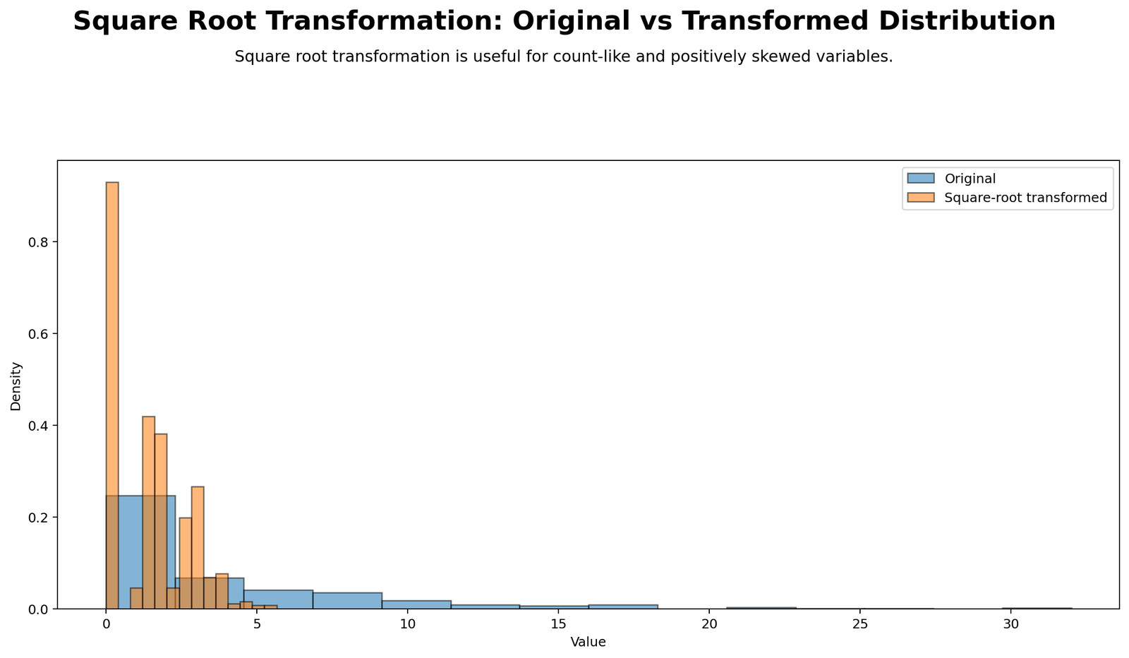
This chart compares the original absences distribution with its square-root transformed version. Before transformation, the distribution is highly right-skewed. Many observations are near zero, and a smaller number extend far to the right up to 32 absences. This creates a long right tail and high skewness.
After square root transformation, the right tail is compressed. The maximum value changes from 32 to about 5.657. The transformed histogram becomes more compact and less dominated by extreme absence counts. This visual result matches the SPSS skewness improvement from 2.021 to .391.
Decision/reporting conclusion: Report that the Python distribution chart supports the use of Square Root Transformation for absences because the transformed distribution is visibly less right-skewed and less dominated by extreme high counts.
Python Chart 2: Q-Q Plot Before and After Square Root Transformation
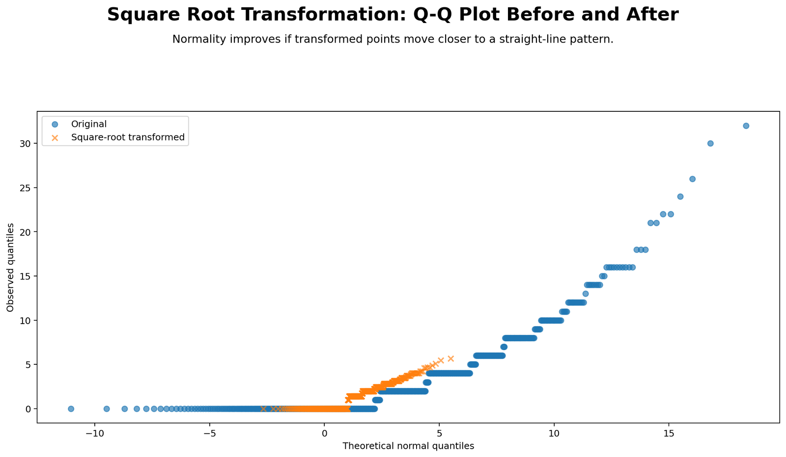
The Q-Q plot shows whether observed values follow the expected normal line. Before transformation, the original absences variable departs strongly from the line, especially in the right tail. This is expected for count data with many low values and a few high values.
After transformation, the Q-Q pattern improves in the central region because extreme high values are compressed. However, the transformed data still do not perfectly follow the normal line. This supports the SPSS normality result: the transformation improves shape, but formal normality is still rejected.
Decision/reporting conclusion: Report that the Q-Q plot shows partial improvement, not perfect normality. For a full guide to interpreting this visual evidence, use the Q-Q plot normality check.
Python Chart 3: Skewness and Kurtosis Before and After
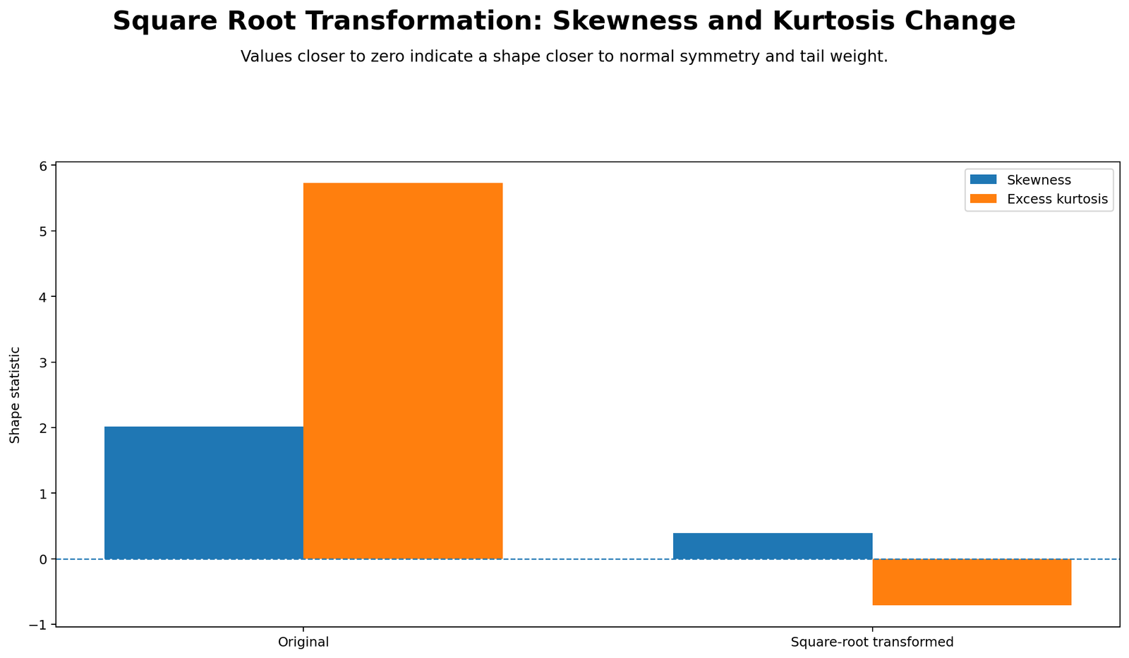
This chart gives the most direct numeric evidence for the transformation benefit. Before transformation, absences has strong positive skewness and high kurtosis. After transformation, skewness moves close to zero and kurtosis becomes much less extreme. The SPSS values confirm this: skewness changes from 2.021 to .391, while kurtosis changes from 5.781 to -.711.
This is the strongest reason to use square root transformation for absences. Even though the normality p-values remain significant, skewness and kurtosis improve substantially. In applied analysis, this can make plots more readable, reduce extreme leverage from high counts, and improve the behavior of some models.
Decision/reporting conclusion: Report that Square Root Transformation was effective for shape improvement because both skewness and kurtosis moved substantially closer to acceptable values.
Python Chart 4: Normality p-values Before and After
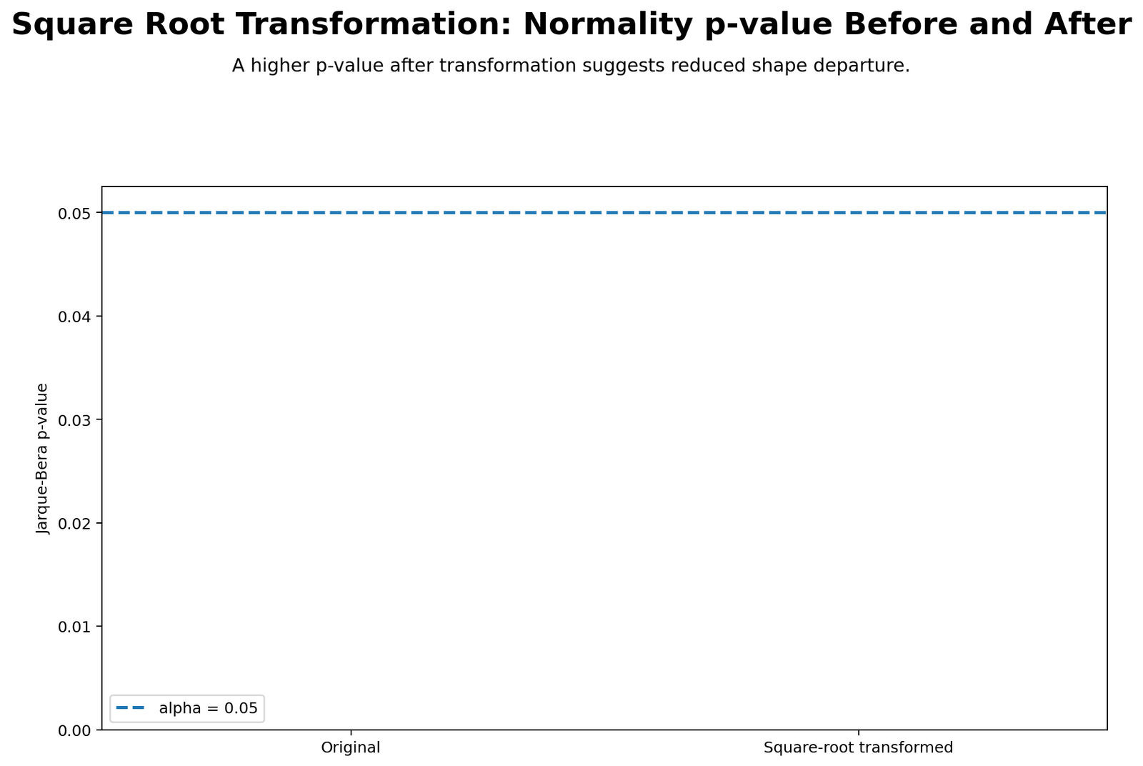
This chart explains why the final conclusion must be careful. The square root transformation improves skewness and kurtosis, but the normality p-values remain very small. In SPSS, both the original absences and transformed sqrt_absences have p < .001 for formal normality tests. Therefore, the transformed variable should not be described as normally distributed.
The correct interpretation is that the transformation improves distribution shape but does not fully satisfy normality. This distinction is important for reports. If a teacher, reviewer, or client asks whether the transformation “worked,” the answer is: it worked for reducing skewness and kurtosis, but it did not make the variable perfectly normal under strict formal tests.
Decision/reporting conclusion: Report that formal normality was still rejected after Square Root Transformation, so the transformation should be described as an improvement rather than a full normality correction.
Python Chart 5: Square Root Transformation Curve
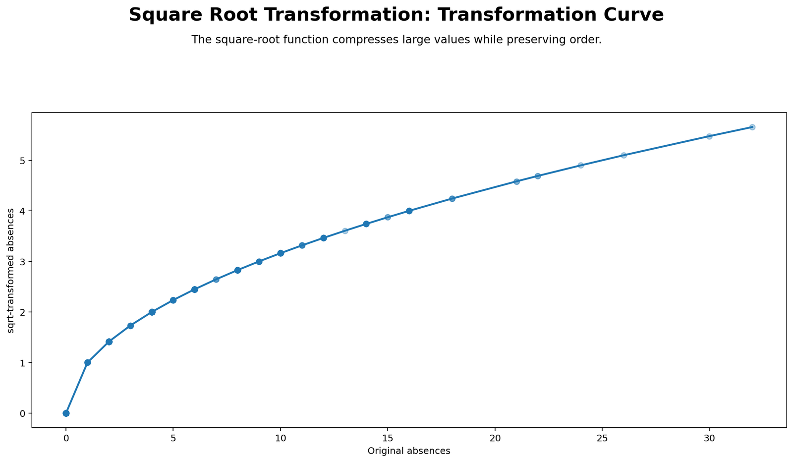
This chart explains the mathematics of the transformation. The square root curve rises quickly at small values and more slowly at large values. That means large raw values are compressed more strongly than small raw values. For example, sqrt(4) = 2, sqrt(16) = 4, and sqrt(32) ≈ 5.657. The raw scale from 0 to 32 becomes a transformed scale from 0 to 5.657.
This compression is why square root transformation is useful for right-skewed count variables. It reduces the influence of large counts without changing the order of the observations. A student with more absences still has a higher transformed value, but the difference is less extreme on the transformed scale.
Decision/reporting conclusion: Report that the transformation curve justifies the method mathematically because it compresses high values while preserving rank order.
Python Chart 6: Group Boxplots Before and After
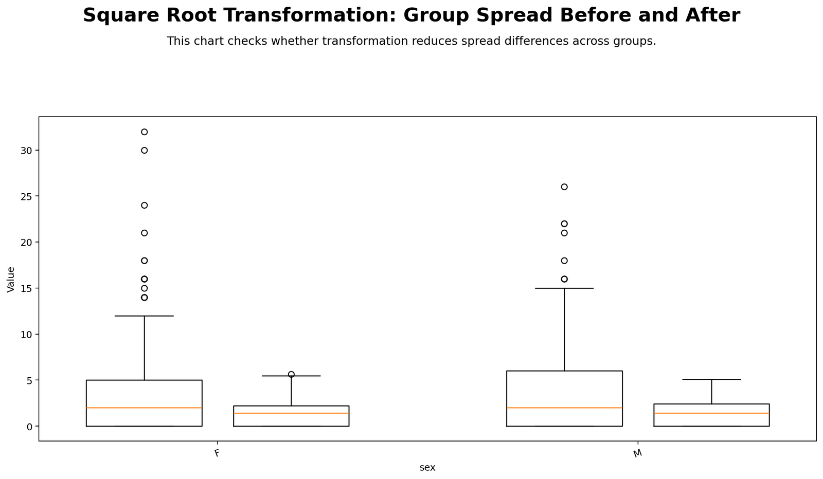
This chart shows the practical effect of transformation across groups. Before transformation, high absence values stretch the boxplots and make group spread harder to compare. After transformation, the scale is compressed, and the group boxes become easier to visually compare. This is useful when the original count variable has a long right tail.
The transformation does not erase group differences or reorder observations. It simply changes the scale so that extreme high values do not dominate the visual display. This makes the transformed boxplots better for comparing distribution shape across groups.
Decision/reporting conclusion: Report that transformed group boxplots are easier to compare visually, but any statistical test should be chosen according to the design, assumptions, and research question. For group spread checks, see Levene’s test and Brown-Forsythe test.
Python Chart 7: Skewness Across Variables
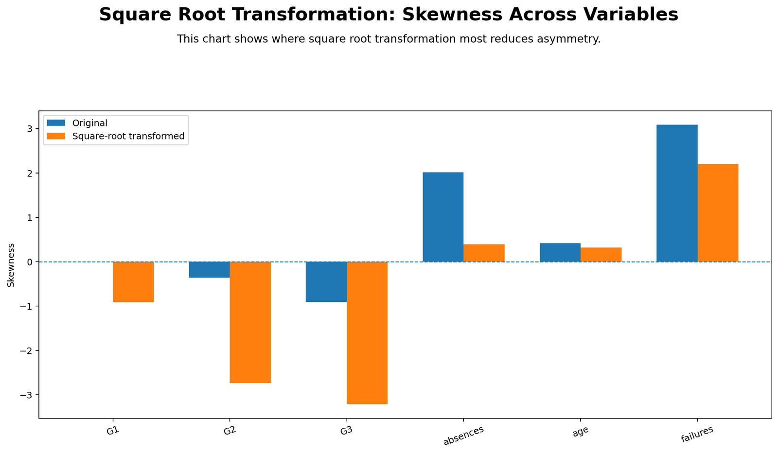
This chart is important because it shows that square root transformation is not equally useful for every variable. Absences improves strongly because it is right-skewed count data. Failures also improves somewhat, but it remains skewed because it has many zero values. Age changes only slightly because it was not highly skewed before transformation. Grade variables such as G3, G2, and G1 may become worse after square root transformation because they are not the best targets for this method.
The final lesson is that transformation must be chosen based on the variable. Do not apply square root transformation automatically to every column. First inspect skewness, histograms, Q-Q plots, measurement scale, and research purpose.
Decision/reporting conclusion: Report that Square Root Transformation should be used selectively. It worked well for absences, partly helped failures, and was not appropriate for every grade variable.
R Chart-by-Chart Validation
The R charts validate the same Square Root Transformation workflow using a separate software environment. The R results confirm the Python and SPSS interpretation: absences improves strongly, while some other variables do not benefit from the transformation.
R Chart 1: Original vs Square Root Distribution
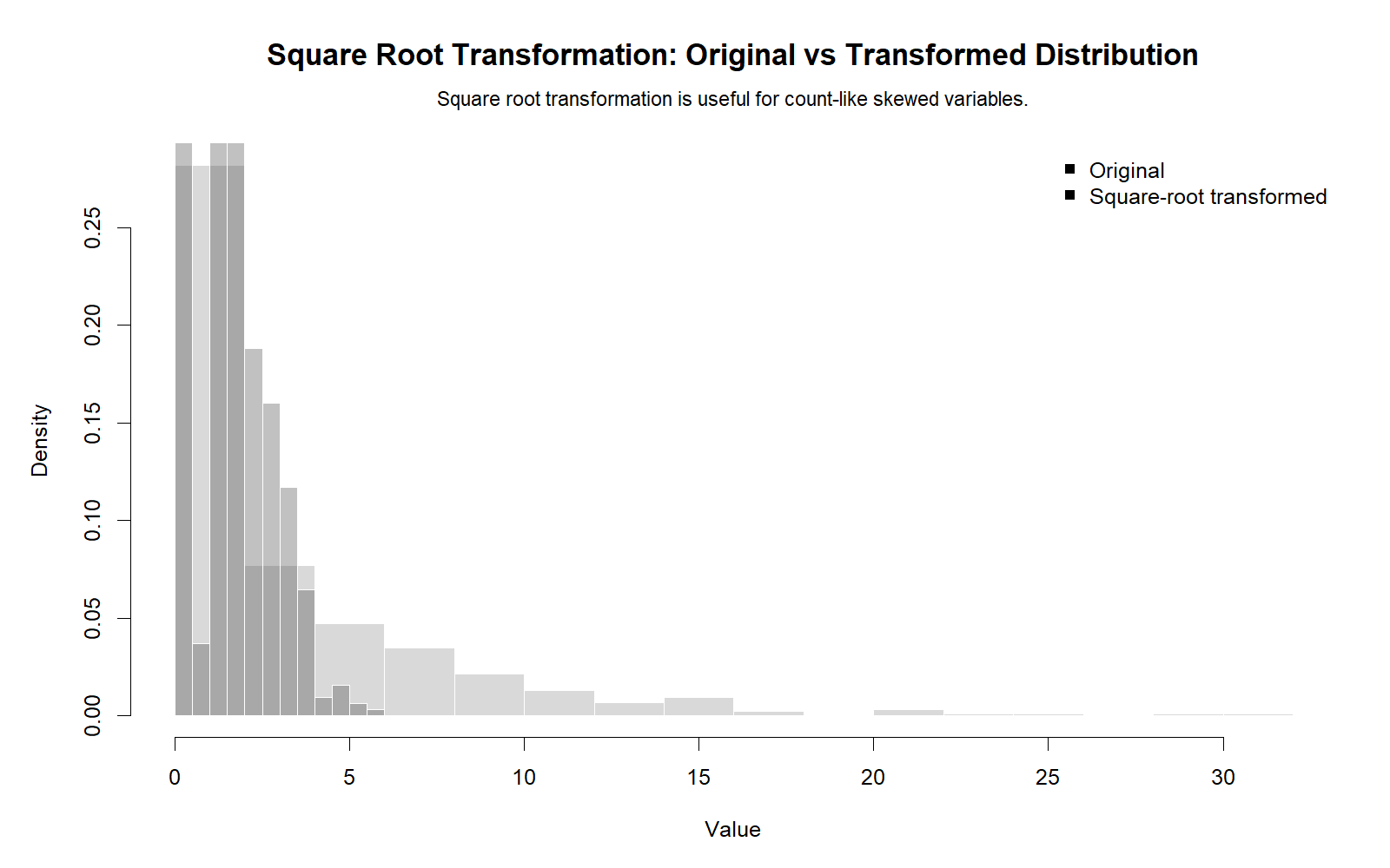
The R distribution chart confirms that the original absences variable is right-skewed and that square root transformation compresses high values. This validates the Python chart and the SPSS descriptives. The transformed distribution becomes more compact, with fewer extreme high-scale values dominating the plot.
Decision/reporting conclusion: Report that the R distribution chart confirms the same improvement shown in Python: the transformed absences variable is less right-skewed and more visually balanced.
R Chart 2: Q-Q Plot Before and After
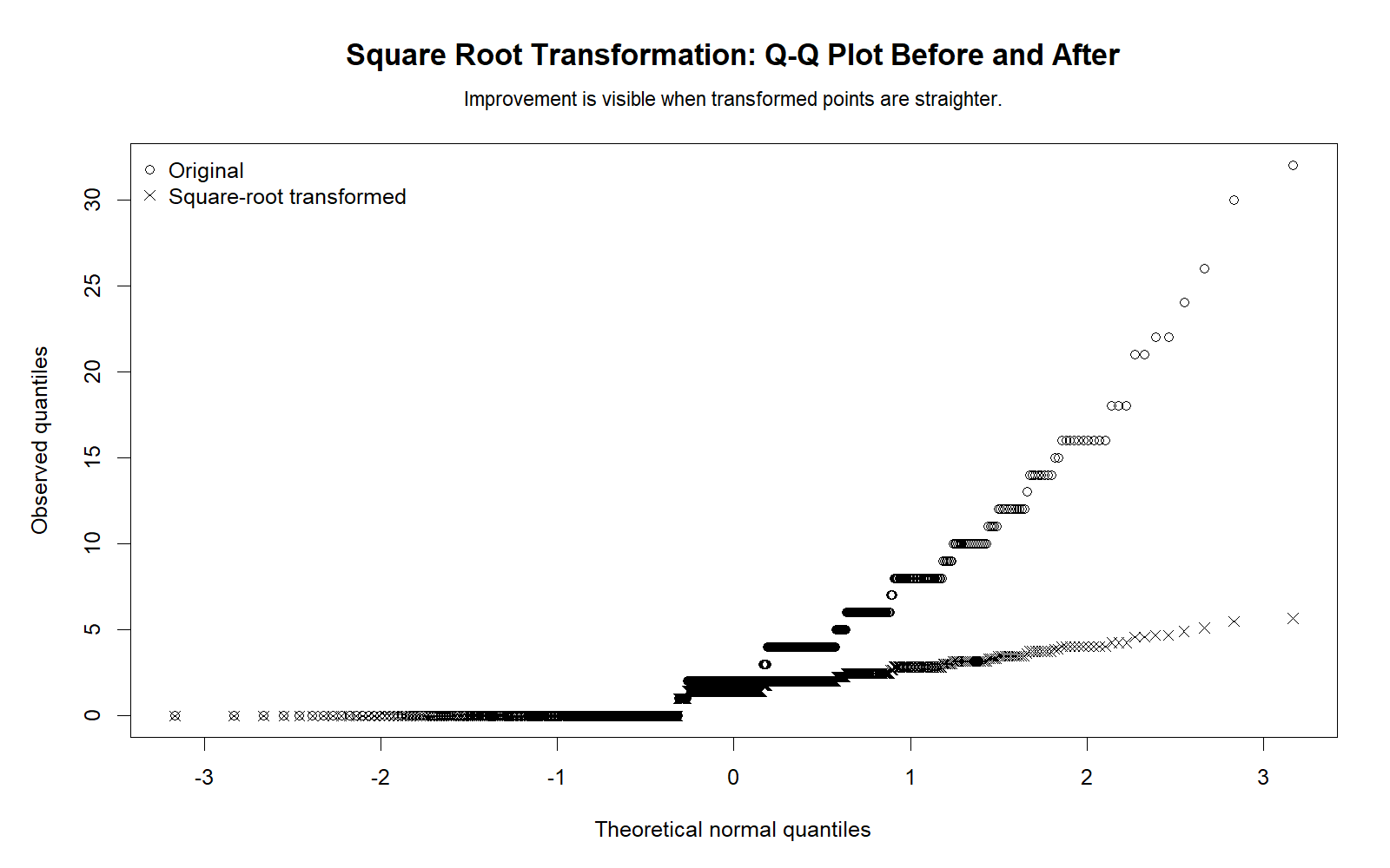
The R Q-Q plot confirms improved central alignment after transformation but still shows departures from normality. This agrees with the SPSS result that normality tests remain significant after transformation. The transformation helps the center of the distribution but cannot fully remove discreteness and zero-heavy features of the count variable.
Decision/reporting conclusion: Report that the R Q-Q plot supports partial normality improvement, but it does not justify saying the transformed variable is perfectly normal.
R Chart 3: Skewness and Kurtosis Before and After
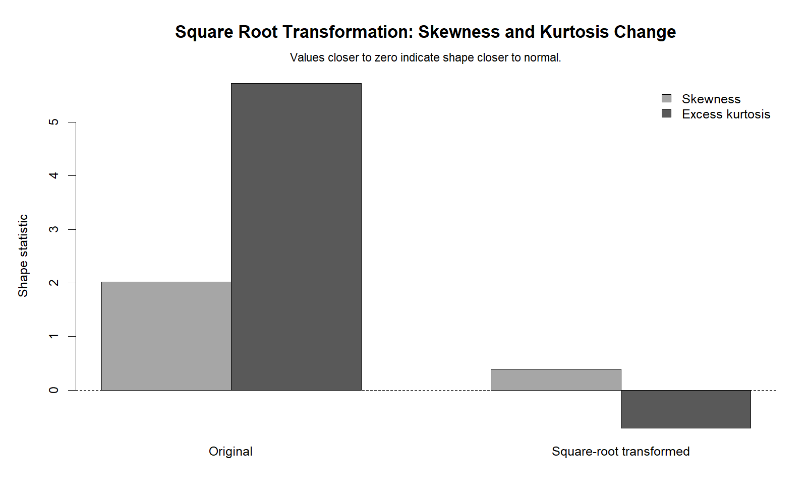
The R skewness-kurtosis chart confirms the main improvement: skewness and kurtosis move much closer to acceptable values for absences. This supports reporting the transformation as successful for shape improvement. The R chart is especially useful because it independently validates the same conclusion produced by SPSS and Python.
Decision/reporting conclusion: Report that R validation confirms a strong reduction in skewness and kurtosis for absences after Square Root Transformation.
R Chart 4: Normality p-values Before and After
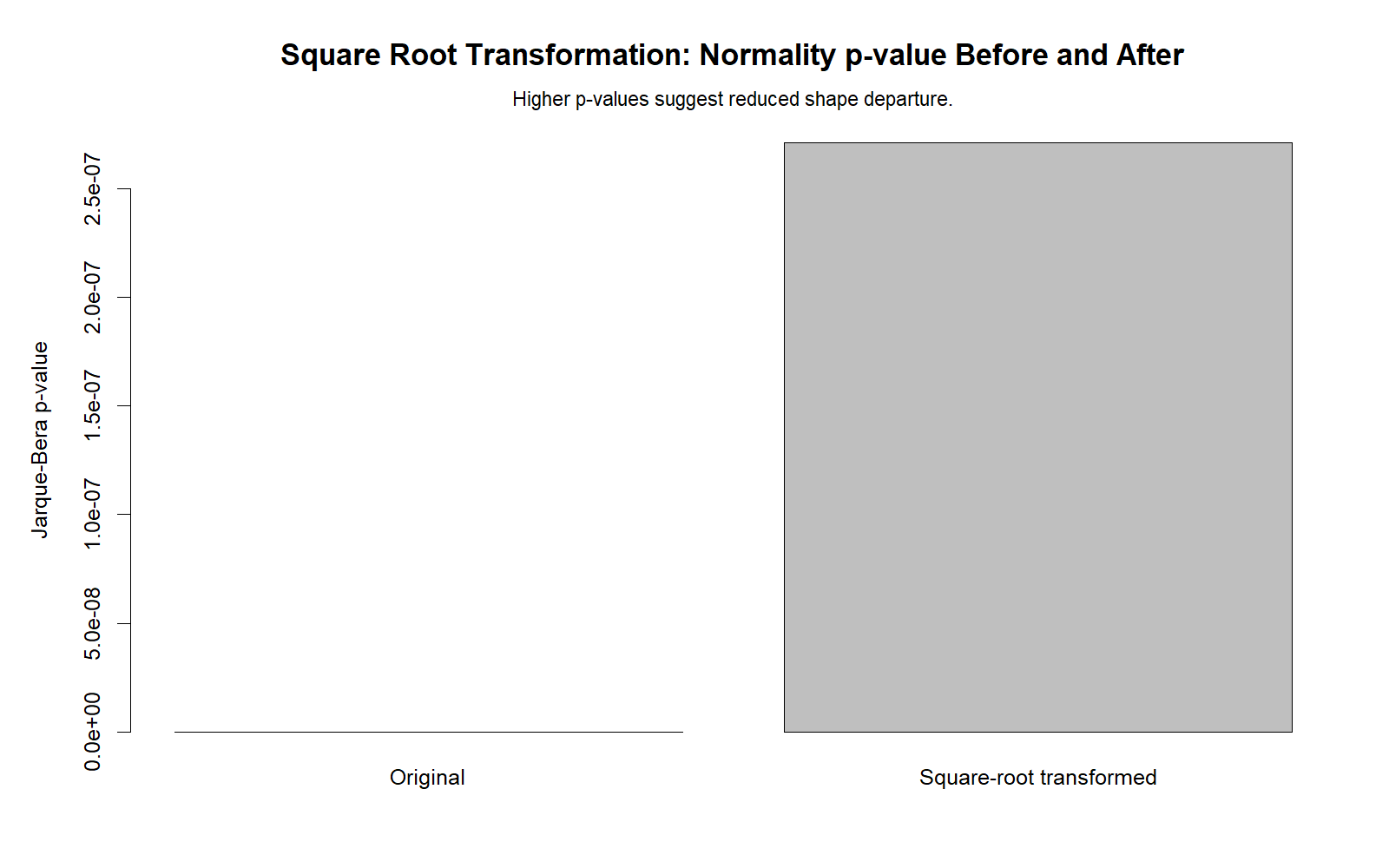
The R normality p-value chart confirms that the transformation does not make the data perfectly normal. It improves descriptive shape, but formal normality tests still reject normality. This is why the report should avoid overstating the transformation result.
Decision/reporting conclusion: Report that the R p-value evidence agrees with SPSS: the transformation improved distribution shape but did not make normality tests non-significant.
R Chart 5: Square Root Transformation Curve
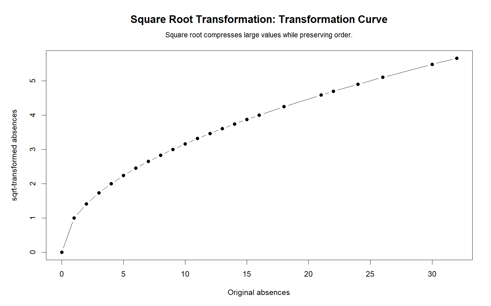
The R transformation curve validates the mathematical explanation. Larger values are compressed more strongly than smaller values. This is the main reason square root transformation reduces right skewness. The curve also shows why the transformation is gentler than a log transformation and often useful for count variables with zeros.
Decision/reporting conclusion: Report that the R transformation curve provides a clear visual explanation of why high absence counts become less extreme on the transformed scale.
R Chart 6: Group Boxplots Before and After
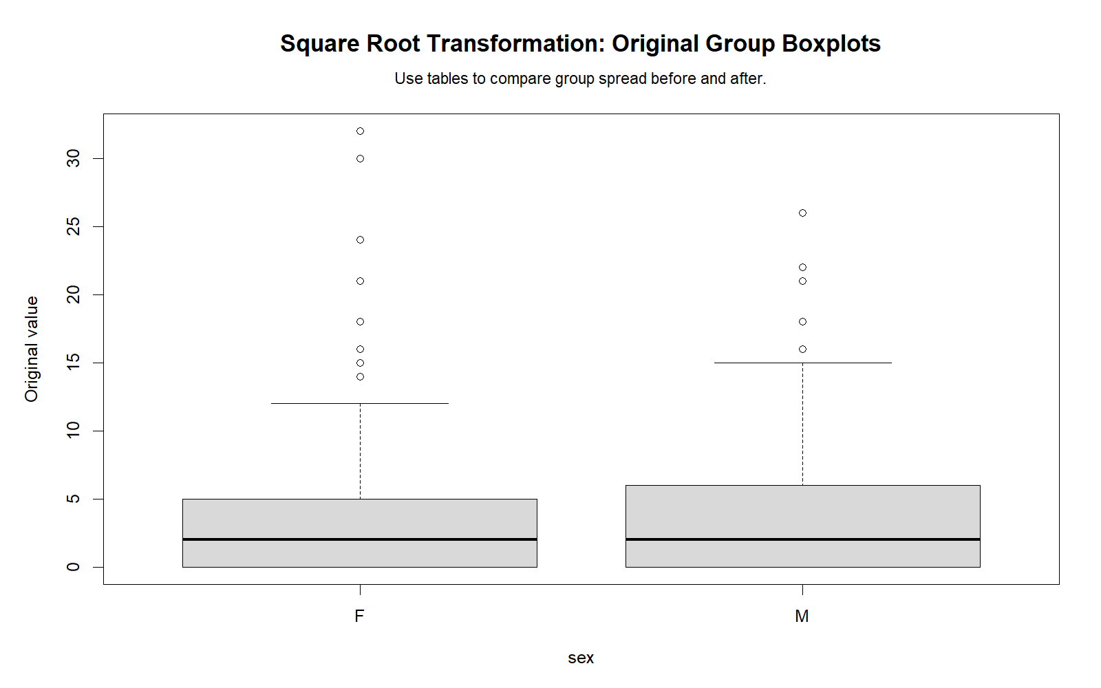
The R group boxplot chart confirms that transformed values are easier to compare visually across groups. Extreme high absence counts have less influence on the plot after transformation. This helps when the analyst wants a clearer descriptive comparison of absence behavior across categories.
Decision/reporting conclusion: Report that R boxplots validate the practical usefulness of transformation for group-level visualization, especially when original count values stretch the vertical scale.
R Chart 7: Skewness Across Variables
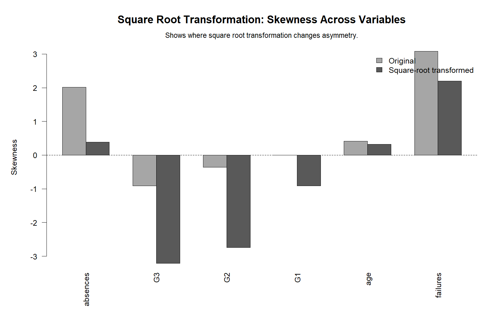
The R skewness-across-variables chart confirms that square root transformation should be applied selectively. Absences improves strongly, failures improves partly, age changes slightly, and several grade variables become less suitable after transformation. This validates the main recommendation: inspect the variable before transforming it.
Decision/reporting conclusion: Report that R validation confirms selective use. Square Root Transformation is appropriate for absences in this dataset but should not be mechanically applied to all variables.
SPSS, R, Python and Excel Workflows for Square Root Transformation
The Square Root Transformation workflow is simple across software. The key steps are to inspect the original variable, calculate the square root, compare skewness and kurtosis before and after, inspect histograms and Q-Q plots, and then decide whether the transformed variable should be used in later analysis.
SPSS Workflow
| Step | SPSS Menu or Syntax | Purpose |
|---|---|---|
| Open dataset | File > Open > Data | Load the SPSS-ready dataset. |
| Inspect original variable | Analyze > Descriptive Statistics > Explore | Check skewness, kurtosis, histogram, Q-Q plot and normality tests. |
| Create transformed variable | Transform > Compute Variable | Use SQRT(absences) to create sqrt_absences. |
| Inspect transformed variable | Explore again | Compare transformed skewness, kurtosis, plots and tests. |
| Decide transformation value | Compare before and after | Use transformation if it improves the analysis purpose. |
| Export output | File > Export or OUTPUT EXPORT | Save SPSS output PDF. |
R Workflow
| Step | R Action | Purpose |
|---|---|---|
| Read data | read.csv() | Load the dataset. |
| Create transformed variable | sqrt_absences <- sqrt(absences) | Apply the transformation. |
| Check shape | skewness(), kurtosis() | Compare shape before and after. |
| Make Q-Q plots | qqnorm(), qqline() | Check normality visually. |
| Run normality test | shapiro.test() where appropriate | Check formal normality evidence. |
| Build charts | Base R or ggplot2 | Create WordPress-ready validation charts. |
Python Workflow
| Step | Python Action | Purpose |
|---|---|---|
| Read data | pandas.read_csv() | Load the dataset into a DataFrame. |
| Create transformed variable | np.sqrt(df["absences"]) | Apply square root transformation. |
| Check shape | scipy.stats.skew(), kurtosis() | Compare skewness and kurtosis before and after. |
| Make Q-Q plots | scipy.stats.probplot() | Compare observed values with normal quantiles. |
| Run normality tests | shapiro(), kstest() | Compare p-values before and after. |
| Create plots | matplotlib | Generate hosted chart images. |
Excel Workflow
| Excel Task | Formula or Tool | Purpose |
|---|---|---|
| Create square root variable | =SQRT(A2) | Transform the original value. |
| Handle zero values | =SQRT(A2) | Zero is allowed because sqrt(0) = 0. |
| Handle negative values | =SQRT(A2-MIN($A$2:$A$650)+1) | Use a shift only if negative values exist. |
| Mean | =AVERAGE(B2:B650) | Calculate transformed mean. |
| Standard deviation | =STDEV.S(B2:B650) | Calculate transformed spread. |
| Histogram | Insert > Statistic Chart > Histogram | Compare distribution shape before and after. |
SPSS Syntax, Python Code, R Code and Excel Formulas
SPSS Syntax for Square Root Transformation
* Square Root Transformation in SPSS.
* Main target variable: absences.

SET PRINTBACK=OFF MPRINT=OFF.

TITLE "Square Root Transformation: Before and After Normality Comparison".

EXAMINE VARIABLES=absences G3 G2 G1 age failures
  /PLOT BOXPLOT HISTOGRAM NPPLOT
  /COMPARE GROUPS
  /STATISTICS DESCRIPTIVES
  /CINTERVAL 95
  /MISSING LISTWISE
  /NOTOTAL.

COMPUTE sqrt_absences = SQRT(absences).
COMPUTE sqrt_G3 = SQRT(G3).
COMPUTE sqrt_G2 = SQRT(G2).
COMPUTE sqrt_G1 = SQRT(G1).
COMPUTE sqrt_age = SQRT(age).
COMPUTE sqrt_failures = SQRT(failures).
EXECUTE.

EXAMINE VARIABLES=sqrt_absences sqrt_G3 sqrt_G2 sqrt_G1 sqrt_age sqrt_failures
  /PLOT BOXPLOT HISTOGRAM NPPLOT
  /COMPARE GROUPS
  /STATISTICS DESCRIPTIVES
  /CINTERVAL 95
  /MISSING LISTWISE
  /NOTOTAL.

OUTPUT SAVE OUTFILE="Square-Root-Transformation-SPSS-Output.spv".

OUTPUT EXPORT
  /CONTENTS EXPORT=VISIBLE
  /PDF DOCUMENTFILE="Square-Root-Transformation-SPSS-Output.pdf".
Python Code for Square Root Transformation
import pandas as pd
import numpy as np
from scipy import stats
import matplotlib.pyplot as plt

df = pd.read_csv("dataset.csv")

x = pd.to_numeric(df["absences"], errors="coerce").dropna()
sqrt_x = np.sqrt(x)

summary = pd.DataFrame({
    "measure": ["mean", "std", "min", "max", "skewness", "kurtosis"],
    "before": [
        x.mean(),
        x.std(ddof=1),
        x.min(),
        x.max(),
        stats.skew(x, bias=False),
        stats.kurtosis(x, fisher=True, bias=False)
    ],
    "after_sqrt": [
        sqrt_x.mean(),
        sqrt_x.std(ddof=1),
        sqrt_x.min(),
        sqrt_x.max(),
        stats.skew(sqrt_x, bias=False),
        stats.kurtosis(sqrt_x, fisher=True, bias=False)
    ]
})

print(summary)

before_shapiro = stats.shapiro(x)
after_shapiro = stats.shapiro(sqrt_x)

print("Before Shapiro-Wilk:", before_shapiro)
print("After Shapiro-Wilk:", after_shapiro)

if abs(stats.skew(sqrt_x, bias=False)) < abs(stats.skew(x, bias=False)):
    print("Square root transformation reduced skewness.")
else:
    print("Square root transformation did not reduce skewness.")

plt.figure(figsize=(10, 6))
plt.hist(x, bins=25, alpha=0.6, label="Original absences")
plt.hist(sqrt_x, bins=25, alpha=0.6, label="Square-root absences")
plt.title("Square Root Transformation: Original vs Transformed Distribution")
plt.xlabel("Value")
plt.ylabel("Frequency")
plt.legend()
plt.tight_layout()
plt.savefig("square_root_transformation_distribution.png", dpi=300)
plt.close()
R Code for Square Root Transformation
# Square Root Transformation in R

df <- read.csv("dataset.csv")

x <- as.numeric(df$absences)
x <- x[!is.na(x)]

sqrt_x <- sqrt(x)

before_summary <- c(
  mean = mean(x),
  sd = sd(x),
  min = min(x),
  max = max(x)
)

after_summary <- c(
  mean = mean(sqrt_x),
  sd = sd(sqrt_x),
  min = min(sqrt_x),
  max = max(sqrt_x)
)

print(before_summary)
print(after_summary)

# Optional package for skewness and kurtosis
# install.packages("moments")
library(moments)

cat("Before skewness:", skewness(x), "\n")
cat("After skewness:", skewness(sqrt_x), "\n")
cat("Before kurtosis:", kurtosis(x) - 3, "\n")
cat("After kurtosis:", kurtosis(sqrt_x) - 3, "\n")

png("square_root_transformation_qq_before.png", width = 1200, height = 900, res = 150)
qqnorm(x, main = "Q-Q Plot Before Square Root Transformation")
qqline(x)
dev.off()

png("square_root_transformation_qq_after.png", width = 1200, height = 900, res = 150)
qqnorm(sqrt_x, main = "Q-Q Plot After Square Root Transformation")
qqline(sqrt_x)
dev.off()

shapiro.test(sqrt_x)
Excel Formulas for Square Root Transformation
Assume original absences values are in A2:A650.

Square root transformation:
=SQRT(A2)

Copy the formula down for all rows.

If negative values exist:
=SQRT(A2-MIN($A$2:$A$650)+1)

Mean before:
=AVERAGE(A2:A650)

Mean after:
=AVERAGE(B2:B650)

Standard deviation before:
=STDEV.S(A2:A650)

Standard deviation after:
=STDEV.S(B2:B650)

Skewness before:
=SKEW(A2:A650)

Skewness after:
=SKEW(B2:B650)

Kurtosis before:
=KURT(A2:A650)

Kurtosis after:
=KURT(B2:B650)

Interpretation:
If skewness moves closer to 0, the transformation improved symmetry.
If kurtosis moves closer to 0, the transformation improved tail/peak behavior.
APA Reporting Wording for Square Root Transformation
When reporting Square Root Transformation, include the reason for transformation, the formula used, the before-and-after skewness/kurtosis values, normality test results, and the final decision about whether the transformed variable was used. If the transformed variable is later used in a group test, regression, or correlation, explain that the analysis was performed on the transformed scale.
APA-Style Transformation Report
The absences variable was positively skewed before transformation, skewness = 2.021, kurtosis = 5.781. A square root transformation was applied using x′ = √x. After transformation, skewness decreased to .391 and kurtosis decreased to -.711, indicating a substantial improvement in distribution shape. However, formal normality tests remained significant for the transformed variable, Kolmogorov-Smirnov D = .240, p < .001, and Shapiro-Wilk W = .880, p < .001. Therefore, the square root transformation improved skewness and kurtosis but did not produce a perfectly normal distribution.
Short Report Sentence
A square root transformation was applied to the absences variable because it was strongly right-skewed. The transformation reduced skewness from 2.021 to .391 and reduced kurtosis from 5.781 to -.711. Although normality tests remained significant, the transformed variable showed a much improved distribution shape.
Student-Friendly Report Example
The absences variable had a long right tail before transformation. After applying the square root transformation, large absence values were compressed, and the distribution became less skewed. The transformation improved the shape of the data, but the formal normality tests still showed p < .001, so the transformed variable should not be described as perfectly normal.
When your final analysis reports hypothesis-test results, also include appropriate effect interpretation. Salar Cafe’s effect size guide and confidence interval guide can help connect transformed-variable analysis with practical interpretation.
Common Mistakes in Square Root Transformation Interpretation
| Mistake | Why It Is a Problem | Correct Practice |
|---|---|---|
| Applying square root transformation to every variable | Some variables become worse after transformation. | Use it mainly for non-negative right-skewed variables. |
| Claiming transformation guarantees normality | Normality tests may still reject after transformation. | Report improvement separately from normality decision. |
| Ignoring zero values | Zero is valid for square root, but log transformation has problems with zero. | Use sqrt(0) = 0 when zero values are present. |
| Using square root on negative values without shifting | The square root of negative numbers is not valid in ordinary real-valued analysis. | Shift the variable or choose another method. |
| Only checking p-values | Large samples can keep p-values significant after improvement. | Check skewness, kurtosis, histograms, Q-Q plots and analysis purpose. |
| Forgetting transformed interpretation | Results are now on the square-root scale. | Explain coefficients, means or plots carefully after transformation. |
| Using transformation to hide outliers | Transformation softens large values but does not explain why they exist. | Investigate extreme cases with boxplots and data checks. |
For outlier and distribution-shape context, use the guides on box plot interpretation, histogram interpretation, frequency distribution, and five-number summary.
Key reminder: Square Root Transformation is a diagnostic and modeling choice. It should be justified with before-and-after evidence, not applied mechanically.
When to Use Square Root Transformation
Use Square Root Transformation when the variable is non-negative, count-based, and positively skewed. It is especially useful when large count values create a long right tail, but the data include zero values that make log transformation less convenient.
| Use Case | Why Square Root Helps | Example from This Guide |
|---|---|---|
| Right-skewed count data | Compresses large values and reduces right tail. | Absences skewness dropped from 2.021 to .391. |
| Data with zeros | sqrt(0) is valid. | Absences minimum stayed 0 before and after. |
| Outlier-softening | Large values become less extreme on the transformed scale. | Maximum absences changed from 32 to 5.6569. |
| Visual comparison | Boxplots and histograms become easier to read. | Group boxplots are less stretched after transformation. |
| Normality improvement | May improve skewness, kurtosis and Q-Q alignment. | Shape improved, but formal normality remained significant. |
For other transformation and assumption topics, compare this guide with reciprocal transformation, Q-Q plot normality check, D’Agostino-Pearson test, Cramer-von Mises test, and Kolmogorov-Smirnov test.
Downloads and Resources for Square Root Transformation
The resources below include the SPSS output PDF, Python charts, and R validation charts used in this guide.
Download SPSS Output PDF
Verified SPSS output for before-and-after square root transformation, skewness, kurtosis, Q-Q plots and normality tests.
Copy Square Root Transformation Code
Use the SPSS, Python, R and Excel code blocks to reproduce the transformation workflow.
Python Chart 1: Original vs Sqrt Distribution
Before-and-after distribution comparison for the transformed variable.
Python Chart 2: Q-Q Plot Before and After
Visual normality comparison before and after transformation.
Python Chart 3: Skewness and Kurtosis
Before-and-after skewness and kurtosis comparison.
R Chart 3: Skewness and Kurtosis
R validation chart for skewness and kurtosis improvement.
FAQs About Square Root Transformation
What is Square Root Transformation?
Square Root Transformation changes each value into its square root. It is mainly used for non-negative right-skewed variables, especially count variables. The formula is x′ = √x.
When should I use Square Root Transformation?
Use it when a variable is non-negative, count-based, and positively skewed. In this guide, absences is a good example because it has many low values and a long right tail.
Can Square Root Transformation handle zero values?
Yes. Square root transformation can handle zero values because sqrt(0) = 0. This is one reason it is convenient for count data with zeros.
Can Square Root Transformation handle negative values?
Not directly in ordinary real-valued analysis. If negative values exist, you must shift the variable first, such as using sqrt(x − minimum + 1), or choose another method.
Did Square Root Transformation make absences normal in this example?
No. It improved skewness and kurtosis strongly, but formal SPSS normality tests still reported p < .001. The correct conclusion is that the transformation improved distribution shape but did not create perfect normality.
What happened to absences skewness after transformation?
Absences skewness decreased from 2.021 before transformation to .391 after square root transformation. This shows a major reduction in positive skewness.
What happened to absences kurtosis after transformation?
Absences kurtosis decreased from 5.781 to -.711. This means the transformed distribution had much less extreme peak and tail behavior.
Should I transform every variable using square root?
No. The output shows that Square Root Transformation helped absences but worsened some grade variables. Always inspect histograms, Q-Q plots, skewness, kurtosis and variable type before transforming.
Is Square Root Transformation better than reciprocal transformation?
It depends on the data. Square root transformation is usually gentler and common for count data. Reciprocal transformation is stronger and can heavily compress large values. Compare both with the Salar Cafe reciprocal transformation guide.
How do I report Square Root Transformation in APA style?
Report the original skewness/kurtosis, the transformation formula, the transformed skewness/kurtosis, normality test results if used, and the decision. For this example, report that skewness improved from 2.021 to .391 and kurtosis improved from 5.781 to -.711, but formal normality remained significant.

