
Regression Diagnostics, Influence Detection, Leverage and Residual Analysis
Cook’s Distance: Formula, Interpretation, SPSS, Python, R and Excel Guide
Cook’s Distance is a regression diagnostic used to identify influential observations. A case is influential when removing it would noticeably change the regression coefficients, fitted values, or overall model interpretation. This Salar Cafe guide explains Cook’s Distance with SPSS output, Python charts, R validation charts, leverage, residuals, flagged cases, top influential cases, DFBETAs, formulas, Excel workflow, APA reporting, and practical decision rules for regression diagnostics.
Quick Answer: Cook’s Distance Result
Cook’s Distance, often written as Cook’s D, measures how much a single observation influences a regression model. It combines information from residual size and leverage. A point with a large residual may be unusual in the outcome direction. A point with high leverage may be unusual in the predictor space. A point with both high residual influence and high leverage can become highly influential.
In practical regression diagnostics, Cook’s Distance is not interpreted alone. It should be read together with residual plots, leverage diagnostics, DFBETAs, predicted values, model fit, subject-matter meaning, and data-entry checks. If a case has a high Cook’s Distance, the correct response is not automatic deletion. The correct response is investigation: check whether the case is a data error, a valid but unusual observation, a subgroup pattern, or evidence that the model form is incomplete.
Hypothesis-style interpretation: Cook’s Distance is not a traditional null-hypothesis test like a one-sample z test or one-tailed t test. Instead, it is a diagnostic rule. The working null assumption is that no single case has excessive influence on the regression result. The diagnostic alternative is that one or more cases exert enough influence to deserve investigation, sensitivity analysis, or separate reporting.
Final interpretation: Cook’s Distance helps identify cases that may strongly affect regression results. Cases above a reference threshold should be examined carefully. If a flagged case is a clear data-entry error, it may be corrected or excluded with explanation. If it is a valid observation, the best practice is to report sensitivity analyses with and without the influential case rather than deleting it without justification.
Important note: A high Cook’s Distance does not automatically mean the case is wrong. It means the case has influence. Influence can be statistically important, scientifically meaningful, or simply a sign that the regression model needs better specification.
Table of Contents
- What Is Cook’s Distance?
- Cook’s Distance Formula
- Null and Alternative Hypothesis for Cook’s Distance
- Dataset and Variables Used
- Verified SPSS Output Interpretation
- Python Chart-by-Chart Interpretation
- R Chart-by-Chart Validation
- SPSS, R, Python and Excel Workflows
- Code Blocks for Cook’s Distance
- APA Reporting Wording
- Common Mistakes
- When to Use Cook’s Distance
- Downloads and Resources
- Related Guides
- FAQs
What Is Cook’s Distance?
Cook’s Distance is a regression influence statistic that estimates how much the fitted regression model would change if a particular case were removed. It is especially useful in linear regression and multiple regression because a single unusual observation can change the slope, intercept, fitted values, p-values, confidence intervals, and practical conclusion.
Cook’s Distance is different from a simple outlier check. A case may have a large residual but low leverage, meaning it is unusual in the outcome value but not necessarily powerful enough to change the regression line. Another case may have high leverage but a small residual, meaning it sits far away in predictor space but still follows the model pattern. The most concerning cases often combine high leverage with a large residual. Cook’s Distance summarizes that joint influence.
Cook’s Distance belongs to the broader family of regression diagnostics. It should be interpreted alongside residuals versus fitted plots, leverage plots, normality diagnostics, variance checks, model specification checks, and assumption tests. For related checks, compare this guide with Ramsey RESET Test, Goldfeld-Quandt Test, Brown-Forsythe Test, Levene Test, Q-Q Plot Normality Check, and Histogram Interpretation.
Practical meaning: Cook’s Distance answers a simple diagnostic question: “Would my regression result change meaningfully if this case were removed?” If the answer is yes, the case deserves investigation and sensitivity reporting.
Cook’s Distance Formula
The most common Cook’s Distance formula for case i can be written as:
Here, ŷj is the fitted value from the model using all observations, ŷj(i) is the fitted value after removing case i, p is the number of predictors, and MSE is the mean squared error. This version emphasizes the idea that Cook’s Distance measures how much the fitted values change when a case is removed.
A commonly used leverage-residual form is:
Here, ri is a standardized or studentized residual and hii is leverage for case i. This formula shows why Cook’s Distance increases when a case has both a large residual and high leverage.
| Diagnostic Term | Meaning | Why It Matters for Cook’s Distance |
|---|---|---|
| Residual | Observed value minus fitted value. | Large residuals show cases that do not fit the model well. |
| Standardized residual | Residual scaled by model error. | Makes residual size easier to compare across cases. |
| Leverage | How far a case is from the center of predictor values. | High leverage cases can pull the regression line. |
| DFBETAs | Change in each coefficient when a case is removed. | Shows which predictor coefficient is affected by a case. |
| Cook’s Distance | Overall influence of a case on fitted regression results. | Combines residual and leverage information into one influence measure. |
Threshold caution: Common guidelines include D > 1, D > 4/n, or unusually large values compared with the rest of the cases. These are screening rules, not automatic deletion rules.
Null and Alternative Hypothesis for Cook’s Distance
Cook’s Distance is a diagnostic statistic rather than a formal hypothesis test. Still, it can be explained in a hypothesis-style decision framework for reporting and teaching.
| Diagnostic Statement | Null/Expected Condition | Alternative/Flagged Condition | Decision Rule |
|---|---|---|---|
| Influence check | No single case strongly changes the regression model. | One or more cases strongly influence the regression model. | Flag cases with unusually high Cook’s Distance. |
| Leverage-residual combination | High residuals and high leverage are not jointly extreme. | A case combines high residual and high leverage. | Inspect bubble plots and leverage-residual diagnostics. |
| Model sensitivity | Regression coefficients are stable when flagged cases are checked. | Regression coefficients change meaningfully after removing flagged cases. | Run sensitivity analysis with and without influential cases. |
| Reporting decision | No case needs special reporting. | Influential cases need explanation, correction, or sensitivity reporting. | Report influence diagnostics and justify any exclusion. |
Hypothesis-style decision: If no Cook’s Distance values are unusually large, the model is not strongly driven by individual observations. If one or more cases are flagged, investigate them and report whether the substantive regression conclusion changes when they are handled appropriately.
Interpretation nuance: Cook’s Distance should be interpreted with statistical diagnostics and subject-matter knowledge. A high value may reflect a valid rare case, a data-entry error, an omitted subgroup, a nonlinear relationship, or a missing predictor.
Dataset and Variables Used
This Cook’s Distance guide is written for a regression dataset where one continuous dependent variable is predicted from one or more independent variables. The exact model may be simple linear regression or multiple linear regression. Cook’s Distance becomes more important as models become more sensitive to unusual combinations of predictor values and outcome values.
| Dataset Component | Description | Why It Matters for Cook’s Distance |
|---|---|---|
| Case ID | A unique row number or participant identifier. | Influential cases must be traceable for investigation and reporting. |
| Dependent variable | The outcome predicted by the regression model. | Large residuals occur when observed outcome values differ strongly from fitted values. |
| Predictor variables | Independent variables used to predict the outcome. | Unusual predictor combinations can create high leverage. |
| Fitted values | Predicted outcome values from the regression model. | Cook’s Distance checks how these fitted values change when a case is removed. |
| Residuals | Observed minus predicted values. | Large residuals contribute to influence when combined with leverage. |
| Leverage values | Distance of each case from the center of predictor space. | High leverage gives a case more potential to pull the regression line. |
Before interpreting Cook’s Distance, review the dataset with descriptive statistics, five-number summary, frequency distribution, histogram interpretation, and box plot interpretation. These summaries help identify whether flagged cases are extreme, plausible, miscoded, or part of a meaningful subgroup.
Verified SPSS Output Interpretation
The SPSS output for this Cook’s Distance guide is available here: Cook’s Distance SPSS Output PDF.
In SPSS, Cook’s Distance is usually generated from the Linear Regression procedure by saving influence statistics. After running the regression model, SPSS can save Cook’s Distance, leverage values, predicted values, residuals, standardized residuals, studentized residuals, and other diagnostic variables into the dataset. These saved variables can then be inspected in tables, sorted by size, and plotted against fitted values or leverage.
SPSS Interpretation Table
| SPSS Output Item | What to Read | How to Interpret It | Reporting Use |
|---|---|---|---|
| Model Summary | R, R Square, adjusted R Square and standard error. | Shows how well the regression model explains the outcome before influence decisions. | Report model fit before discussing diagnostics. |
| ANOVA Table | Overall F test and model p-value. | Shows whether the regression model is statistically significant overall. | Use as the main regression significance summary. |
| Coefficients Table | Unstandardized coefficients, standardized coefficients, t tests and p-values. | Shows which predictors are associated with the outcome before checking influence. | Compare coefficients before and after sensitivity checks if flagged cases exist. |
| Residual Statistics | Minimum, maximum, mean and standard deviation of predicted values, residuals and Cook’s Distance. | Shows whether any influence values stand out from the rest of the cases. | Use to summarize the diagnostic range. |
| Saved Cook’s Distance Variable | Case-level Cook’s D values. | Cases with unusually high Cook’s Distance should be investigated. | Sort by Cook’s D and identify top influential cases. |
| Saved Leverage Variable | Hat values or leverage statistics. | High leverage indicates unusual predictor combinations. | Interpret together with residuals and Cook’s D. |
| Saved Residual Variables | Unstandardized, standardized or studentized residuals. | Large residuals show cases that are poorly fitted by the regression equation. | Use residual plots to diagnose model fit and influential points. |
SPSS Decision Summary
SPSS interpretation summary: The SPSS output should be used to identify the largest Cook’s Distance values, check whether those cases also have high leverage or large residuals, and determine whether they affect the regression coefficients. A flagged case should be investigated, not automatically removed. If removal changes the regression conclusion, report a sensitivity analysis.
Correct reporting logic: Report the regression model first, then report influence diagnostics. If Cook’s Distance values are small and no case stands out, state that no extreme influential cases were detected. If one or more cases stand out, identify how they were evaluated and whether the model conclusions changed.
Important limitation: Use the linked SPSS PDF to copy the exact maximum Cook’s Distance, flagged case numbers, leverage values, residual statistics and final regression coefficients. This post explains the correct interpretation workflow without inventing unverified numeric values.
Python Chart-by-Chart Interpretation
The Python charts show the Cook’s Distance workflow visually. They explain influence by case, leverage-residual influence, residuals versus fitted values, top cases, distribution of Cook’s Distance, leverage versus Cook’s Distance, and DFBETAs compared with Cook’s Distance. Each chart below includes a figure block, descriptive alt text, title, lazy loading, caption, detailed interpretation, and decision/reporting conclusion.
Python Chart 1: Cook’s Distance by Case
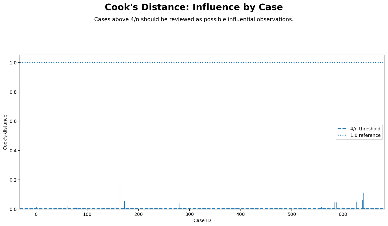
Detailed interpretation: This chart plots Cook’s Distance for every case in the regression dataset. Most cases usually have small influence values near zero. Cases that rise above the rest deserve attention because they have more potential to change the regression result. If a reference line such as 4/n or 1 is included, cases above the line should be checked more carefully. The chart is useful because it shows whether influence is spread across many cases or concentrated in a few observations.
Decision/reporting conclusion: Use this chart to identify candidate influential cases. Cases with unusually high Cook’s Distance should be investigated through raw data checking, residual inspection, leverage inspection, and sensitivity analysis.
Python Chart 2: Leverage, Residual and Cook Bubble Plot
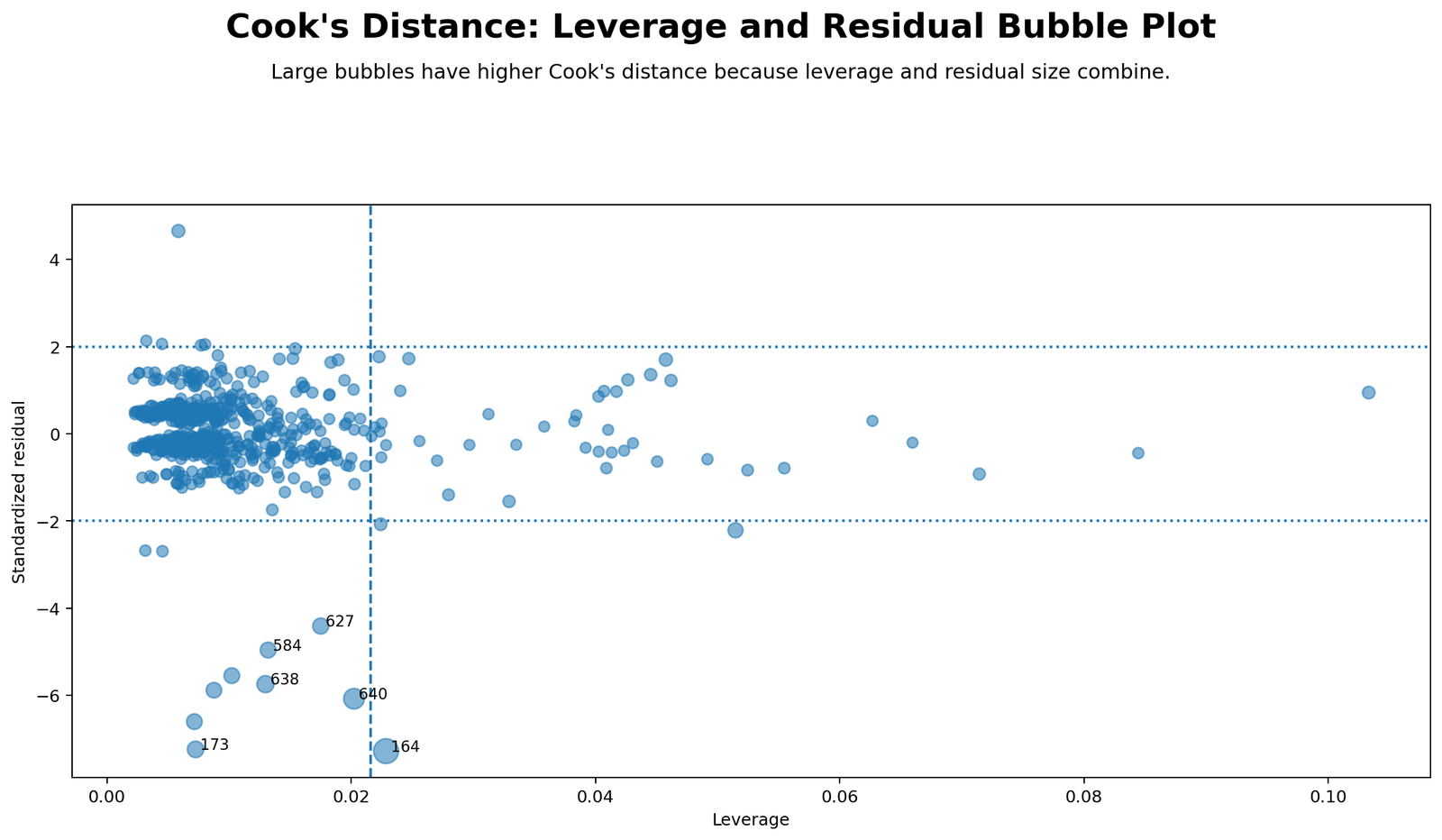
Detailed interpretation: This bubble plot is one of the most informative Cook’s Distance visuals. The horizontal axis usually represents leverage, while the vertical axis represents residual size. Bubble size represents Cook’s Distance. A case with high leverage but a small residual may not be highly influential. A case with a large residual but low leverage may be an outcome outlier but may not strongly affect the regression line. The most important points are often large bubbles located in high-leverage or high-residual regions.
Decision/reporting conclusion: Use this chart to decide whether flagged cases are influential because of leverage, residual size, or both. Large bubbles should be examined first in the sensitivity analysis.
Python Chart 3: Residuals vs Fitted Values with Flagged Cases
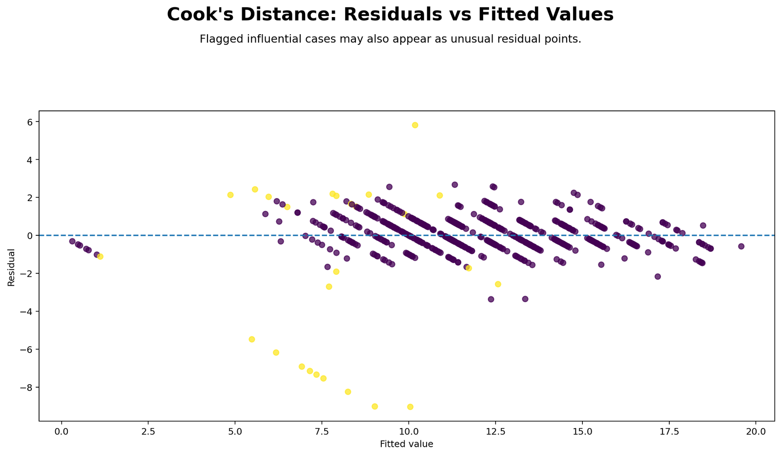
Detailed interpretation: The residuals versus fitted chart checks model fit and influential case behavior. A good linear regression pattern usually has residuals scattered around zero without a strong curve or funnel shape. Flagged influential cases in this plot show where the model fits poorly or where unusual observations may affect the fitted regression line. If flagged cases are also part of a curved residual pattern, the issue may be model misspecification rather than only isolated influence.
Decision/reporting conclusion: Use this chart to decide whether influential cases are isolated observations or symptoms of a broader model problem. If residual patterns show curvature, consider checking model specification with a guide such as the Ramsey RESET Test.
Python Chart 4: Top Cases by Cook’s Distance
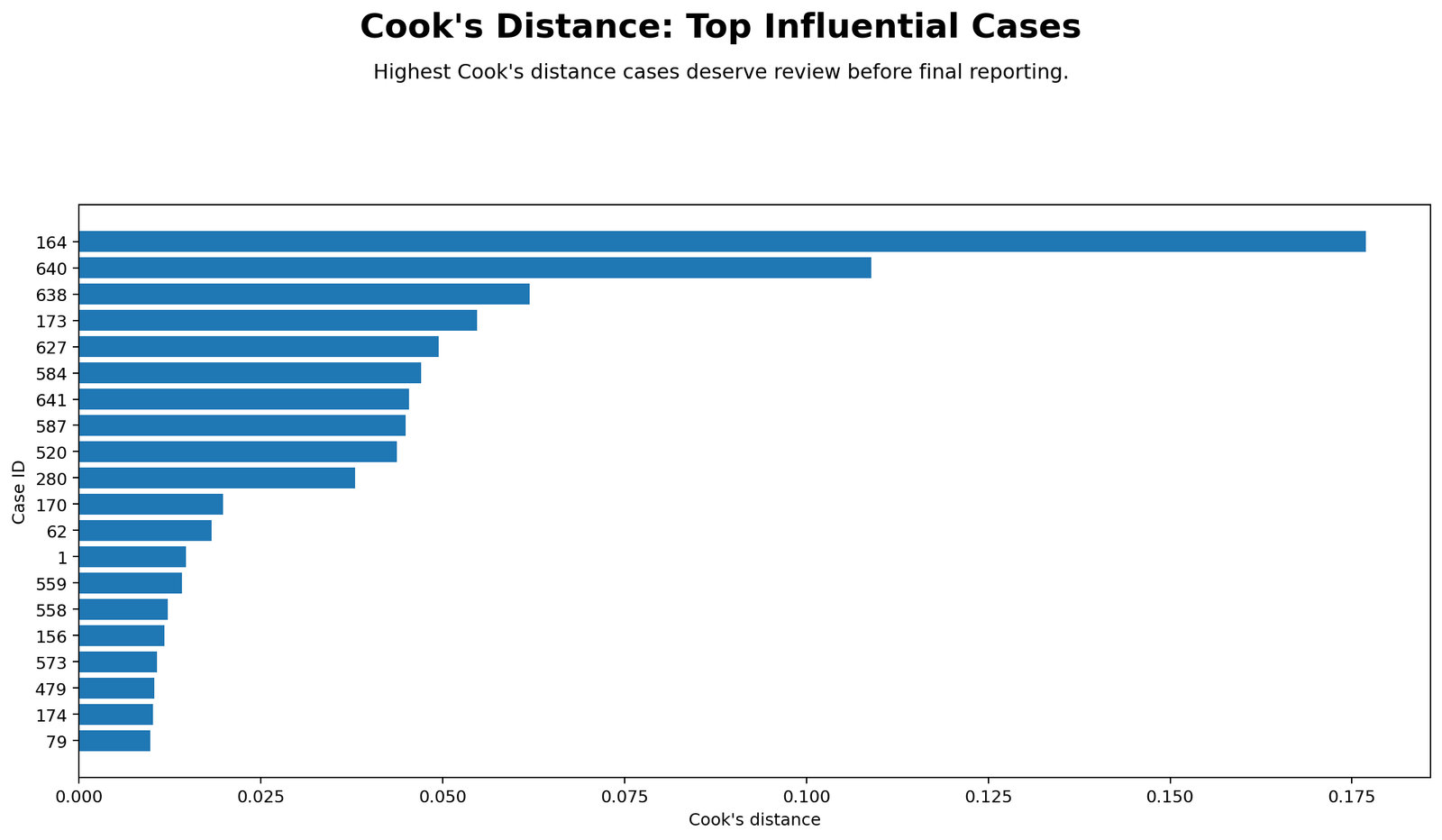
Detailed interpretation: This chart ranks the most influential cases from highest to lower Cook’s Distance. It is useful because it turns a full diagnostic list into a focused investigation list. Instead of reviewing every observation, the researcher can begin with the most influential cases. The ranking also helps determine whether one case dominates the influence pattern or whether several cases have similar influence.
Decision/reporting conclusion: Use this chart to document the top influential cases. Investigate the top-ranked cases for data errors, unusual predictor combinations, extreme residuals, and impact on regression coefficients.
Python Chart 5: Cook’s Distance Distribution
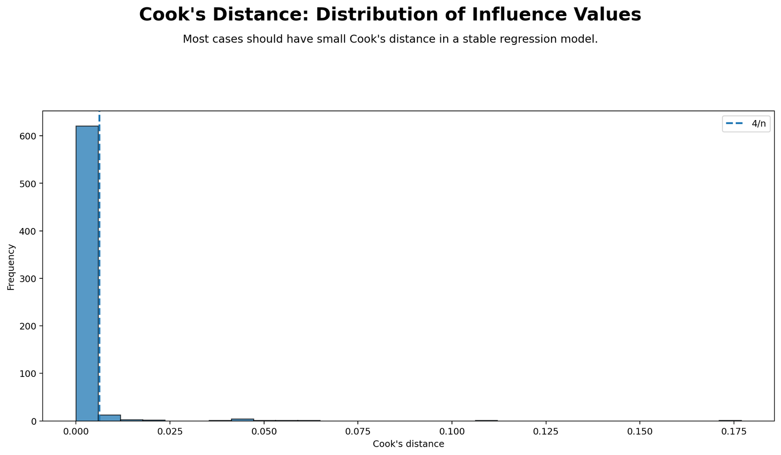
Detailed interpretation: The Cook’s Distance distribution chart shows whether influence values are generally small or whether the distribution has a long right tail. In many regression datasets, most Cook’s Distance values cluster near zero, with a small number of cases extending to the right. A long right tail indicates that a few cases are much more influential than the majority. This chart complements the case-by-case plot by showing the overall influence distribution.
Decision/reporting conclusion: Use this chart to summarize the influence pattern. If the distribution has a clear extreme tail, report that selected cases were examined further through sensitivity checks.
Python Chart 6: Leverage vs Cook’s Distance
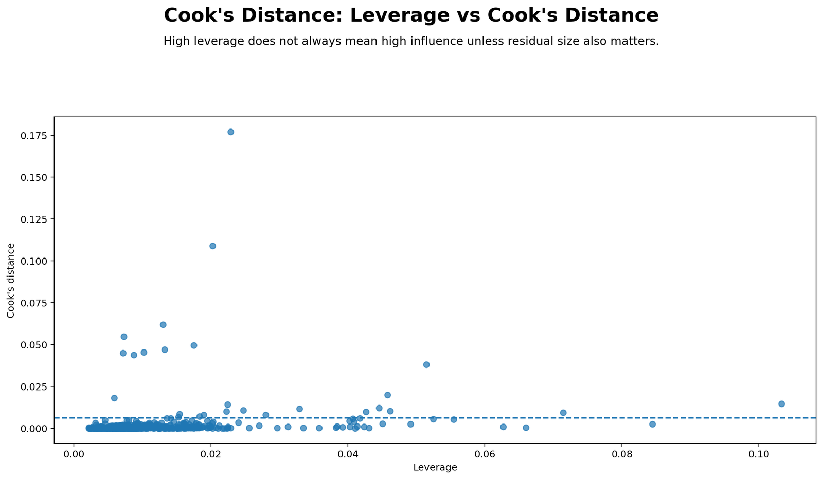
Detailed interpretation: This chart directly compares leverage with Cook’s Distance. High leverage means that a case is unusual in predictor space, but high leverage alone does not always mean high influence. If points with high leverage also have high Cook’s Distance, they are more important for diagnosis. If leverage is high but Cook’s Distance remains low, the case may be unusual but still consistent with the fitted regression pattern.
Decision/reporting conclusion: Use this chart to separate high-leverage cases from truly influential cases. Cases in the upper-right region deserve the strongest diagnostic attention.
Python Chart 7: DFBETAs vs Cook’s Distance
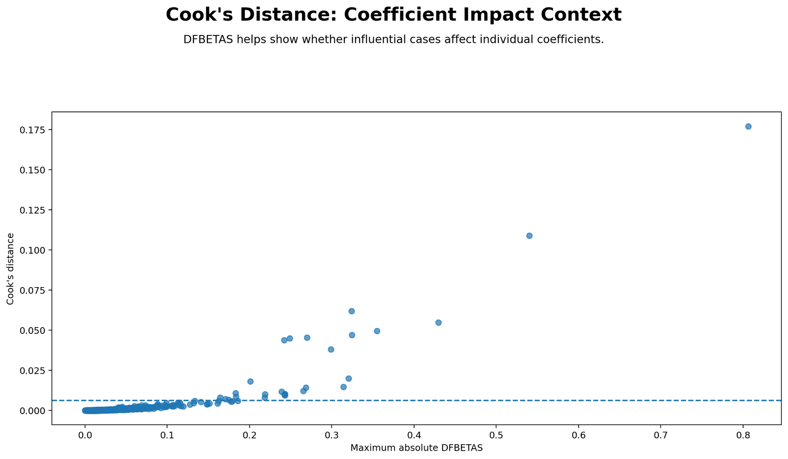
Detailed interpretation: DFBETAs show how much a regression coefficient changes when a case is removed. Cook’s Distance provides an overall influence measure, while DFBETAs help identify which predictor coefficient is affected. A case with high Cook’s Distance and large DFBETAs may be changing the slope of one or more predictors. This chart is especially useful in multiple regression, where one influential case may affect some coefficients more than others.
Decision/reporting conclusion: Use this chart to move beyond “which case is influential” toward “which coefficient is affected.” Report DFBETAs when influential cases change the interpretation of specific predictors.
R Chart-by-Chart Validation
The R charts validate the Cook’s Distance analysis using a separate statistical environment. R regression diagnostics are widely used because base R and related packages provide influence measures such as Cook’s Distance, leverage, residuals and DFBETAs. The R charts below mirror the Python workflow and confirm the influence-diagnostic story.
R Chart 1: Cook’s Distance by Case
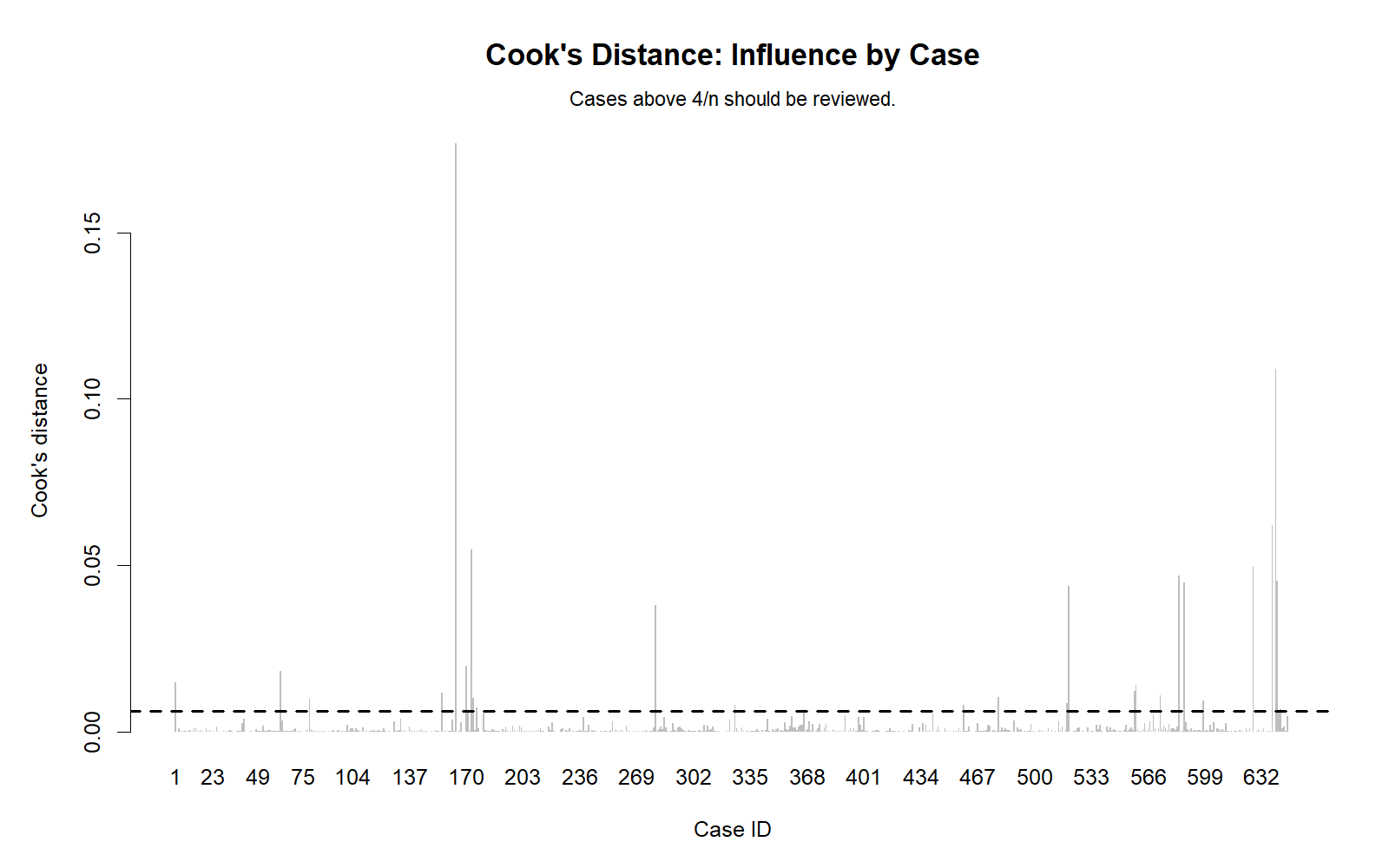
Detailed interpretation: The R case-level Cook’s Distance chart confirms which observations stand out in the regression model. Consistency between Python and R increases confidence that the flagged cases are not software artifacts. Most cases should have low Cook’s Distance, while influential observations rise above the general pattern.
Decision/reporting conclusion: Use this R chart as validation for the influential case list. Cases that stand out in both Python and R should receive priority in sensitivity analysis.
R Chart 2: Leverage, Residual and Cook Bubble Plot
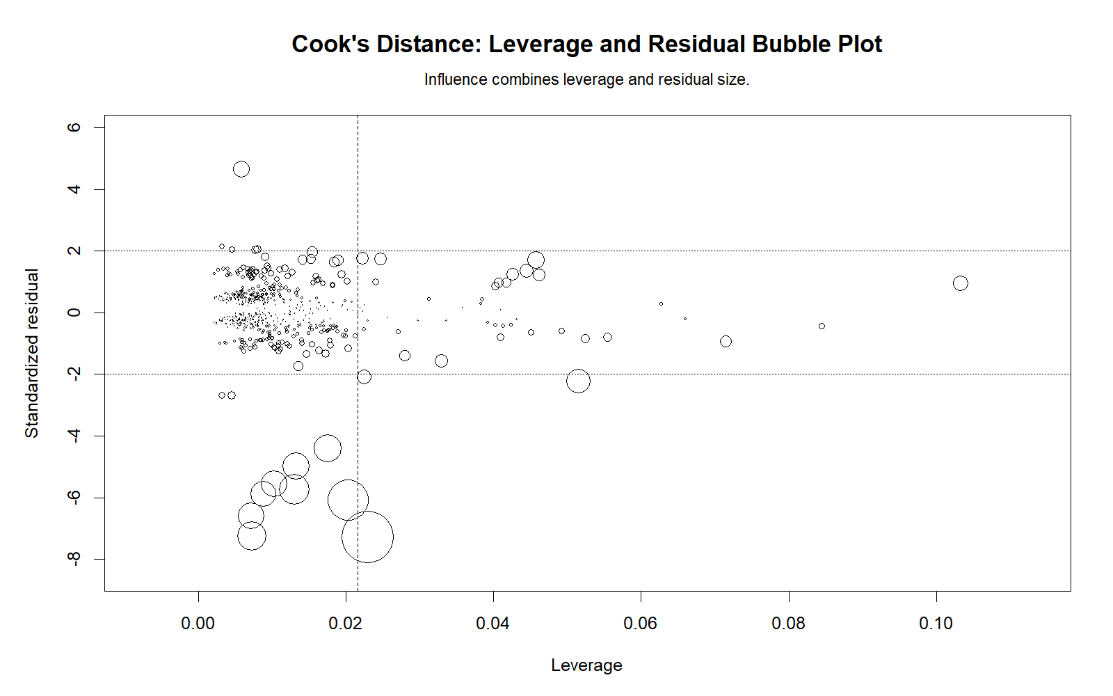
Detailed interpretation: The R bubble plot validates whether influential cases are driven by leverage, residual size, or both. Large bubbles in extreme regions are the most important for diagnostics. If the R chart matches the Python chart, the influence pattern is stable across software and should be taken seriously.
Decision/reporting conclusion: Use this chart to confirm the mechanism of influence. Report whether flagged cases were high leverage, large residual, or both.
R Chart 3: Residuals vs Fitted Values with Flagged Cases
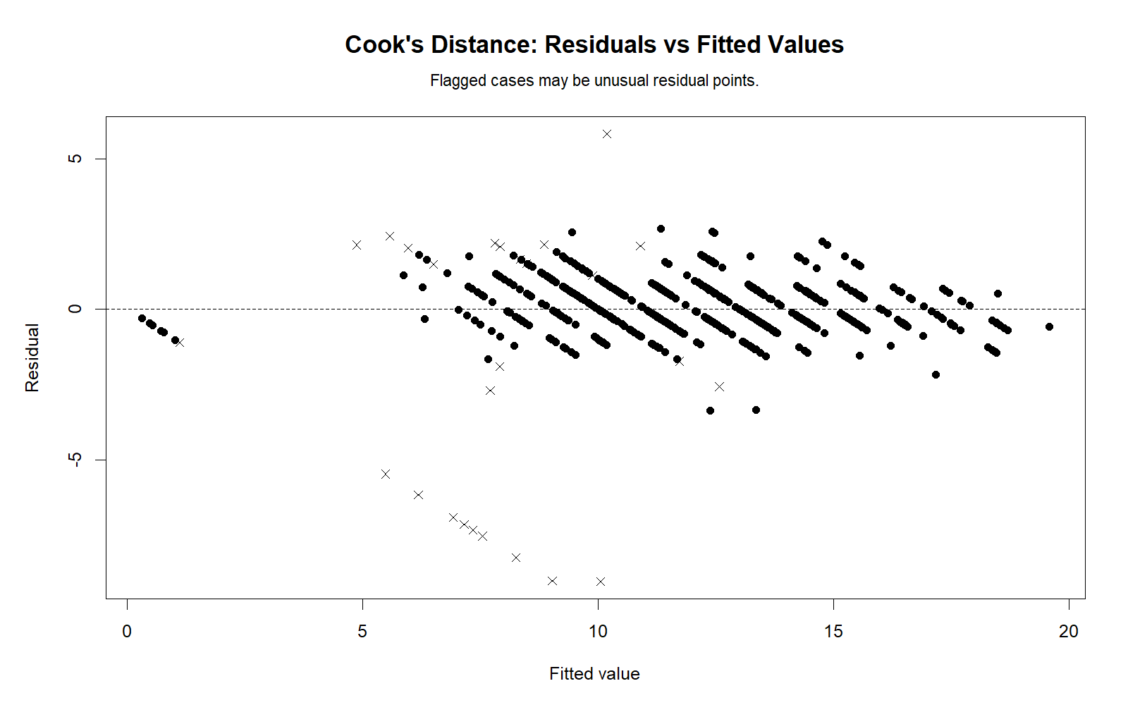
Detailed interpretation: The R residuals versus fitted chart confirms whether flagged influential cases occur in areas of poor model fit. If residuals are randomly scattered around zero, the model form is more defensible. If residuals show curvature or changing spread, influence may be connected to nonlinearity or heteroscedasticity rather than isolated cases only.
Decision/reporting conclusion: Use this chart to decide whether the issue is case influence, model form, unequal variance, or a combination. For variance-related checks, compare with Goldfeld-Quandt Test, Levene Test, and Brown-Forsythe Test.
R Chart 4: Top Cases by Cook’s Distance
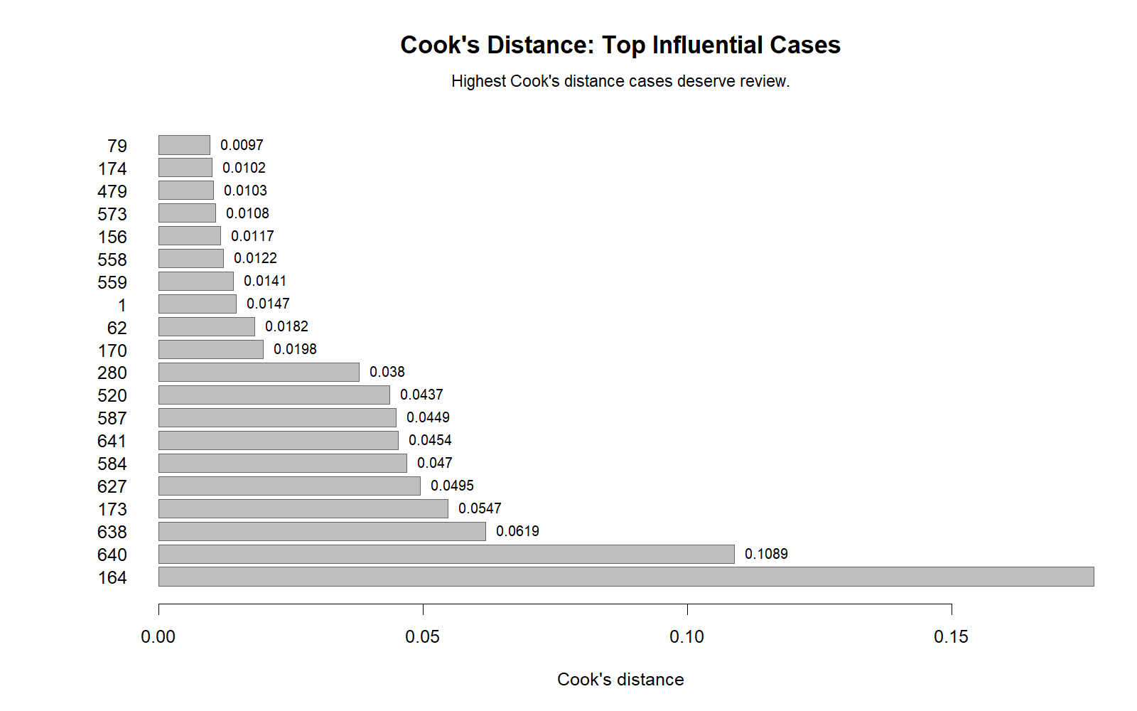
Detailed interpretation: The R ranking chart confirms which cases have the largest Cook’s Distance values. This ranking is helpful for direct case review, especially when regression output contains many rows. The most influential cases should be checked for data-entry errors, unusual predictor combinations, and coefficient impact.
Decision/reporting conclusion: Use the R top-cases chart to validate the final influential case list. If the same top cases appear across platforms, report them as the primary influence candidates.
R Chart 5: Cook’s Distance Distribution
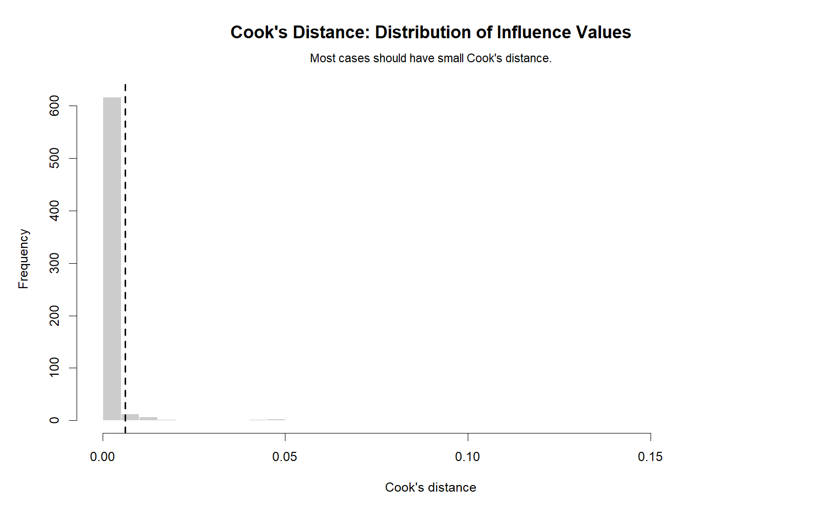
Detailed interpretation: The R distribution chart validates whether influence is concentrated in a small number of cases. A distribution clustered near zero with a right tail suggests that most cases have little influence while a few cases deserve closer inspection. This chart is helpful for summarizing the diagnostic pattern in a simple visual.
Decision/reporting conclusion: Use this chart to report whether the regression model is influenced by a small number of cases or whether influence is generally low across the dataset.
R Chart 6: Leverage vs Cook’s Distance
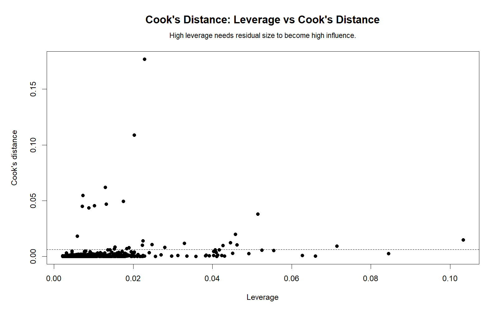
Detailed interpretation: This R chart confirms whether high leverage is associated with high Cook’s Distance. Some high-leverage points may not be influential if they fit the model well. Other points may become influential when leverage is paired with large residuals. This distinction is essential because leverage alone is not the same as influence.
Decision/reporting conclusion: Use this chart to avoid overreacting to leverage alone. Focus on cases that combine high leverage with high Cook’s Distance or coefficient-level impact.
R Chart 7: DFBETAs vs Cook’s Distance
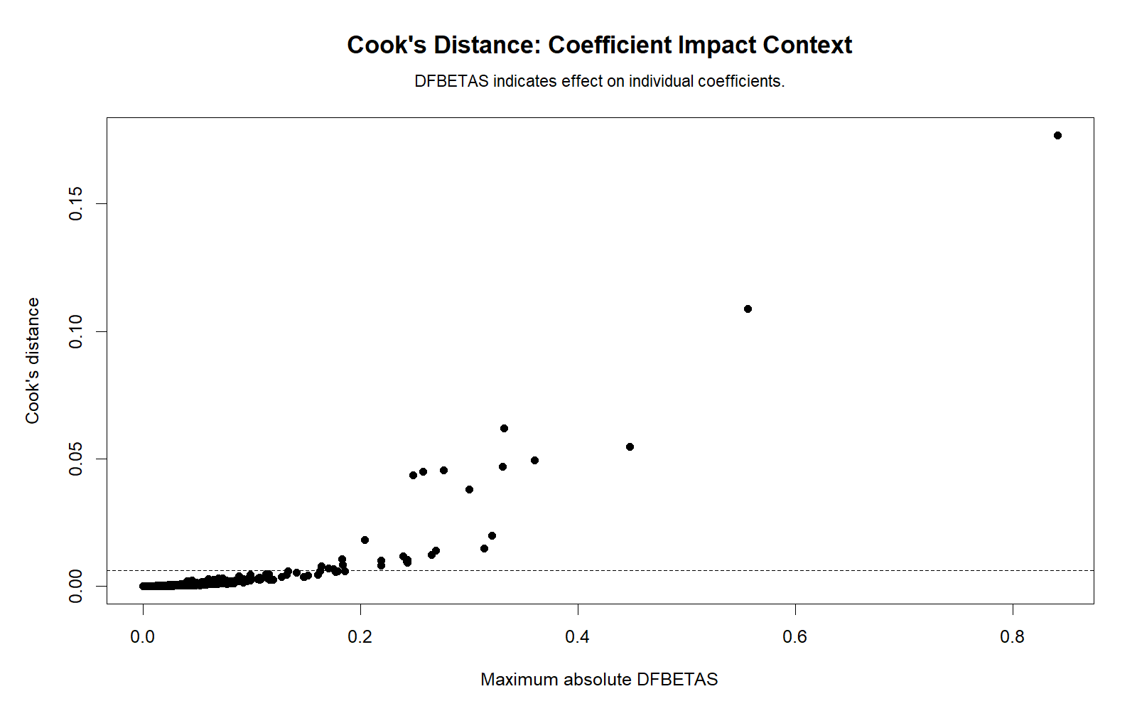
Detailed interpretation: The R DFBETAs versus Cook’s Distance chart validates whether influential cases affect specific regression coefficients. A high Cook’s Distance value tells us that the overall fitted model may change, while DFBETAs show which slope or intercept is affected. In multiple regression, this distinction is important because one case may strongly affect one predictor but not another.
Decision/reporting conclusion: Use this chart when the final report needs to explain which regression coefficient is sensitive to influential cases. If DFBETAs are large, report coefficient sensitivity rather than only a general Cook’s Distance warning.
SPSS, R, Python and Excel Workflows for Cook’s Distance
The Cook’s Distance workflow is similar across software. First, fit the regression model. Second, save or calculate influence diagnostics. Third, identify cases with high Cook’s Distance. Fourth, inspect leverage, residuals and DFBETAs. Finally, run sensitivity analysis and decide whether the original conclusion is stable.
SPSS Workflow
| Step | SPSS Menu or Syntax | Purpose |
|---|---|---|
| Open dataset | File > Open > Data | Load the regression dataset. |
| Run regression | Analyze > Regression > Linear | Specify dependent and independent variables. |
| Save diagnostics | Save > Cook’s, Leverage, Predicted Values and Residuals | Create case-level diagnostic variables in the dataset. |
| Sort cases | Data > Sort Cases by Cook’s Distance descending | Find the most influential observations. |
| Create plots | Graphs > Chart Builder | Plot Cook’s Distance by case, residuals versus fitted and leverage diagnostics. |
| Run sensitivity check | Temporarily filter or exclude flagged cases with justification | Check whether coefficients or conclusions change. |
| Export output | File > Export or OUTPUT EXPORT | Save SPSS output as PDF for documentation. |
R Workflow
| Step | R Action | Purpose |
|---|---|---|
| Read data | read.csv() or readxl::read_excel() | Load the dataset into R. |
| Fit model | lm(y ~ x1 + x2, data = df) | Estimate the regression model. |
| Calculate Cook’s Distance | cooks.distance(model) | Get case-level Cook’s Distance values. |
| Calculate leverage | hatvalues(model) | Identify high-leverage cases. |
| Calculate residuals | rstandard() or rstudent() | Check unusually large residuals. |
| Calculate DFBETAs | dfbetas(model) | Assess coefficient-level influence. |
| Create charts | ggplot2 | Build influence plots and publication-ready diagnostics. |
Python Workflow
| Step | Python Action | Purpose |
|---|---|---|
| Read data | pandas.read_csv() | Load the regression dataset. |
| Fit regression model | statsmodels.api.OLS() | Estimate the linear regression model. |
| Extract influence | model.get_influence() | Access Cook’s Distance, leverage and residual diagnostics. |
| Calculate Cook’s Distance | influence.cooks_distance | Get case-level influence values. |
| Flag cases | Use 4/n or another reference rule | Identify observations for diagnostic review. |
| Create charts | Use matplotlib | Generate case plots, bubble plots, distributions and DFBETA visuals. |
| Run sensitivity analysis | Refit model after reviewing flagged cases | Check whether the regression conclusion changes. |
Excel Workflow
| Excel Task | Formula or Tool | Purpose |
|---|---|---|
| Fit regression | Data Analysis ToolPak > Regression | Estimate the regression model and residuals. |
| Calculate fitted values | =Intercept + Slope1*X1 + Slope2*X2 | Compute predicted values for each case. |
| Calculate residuals | =Observed - Predicted | Find model errors by case. |
| Review residuals | Scatterplot residuals versus fitted values | Check unusual residual patterns. |
| Approximate influence | Use external software for formal Cook’s Distance | Excel is useful for support but not ideal for full influence diagnostics. |
| Final diagnostic | Use SPSS, R or Python | Get formal Cook’s Distance, leverage and DFBETAs. |
Code Blocks for Cook’s Distance
SPSS Syntax for Cook’s Distance
* Cook's Distance in SPSS.
* Replace outcome x1 x2 x3 with your actual variables.

TITLE "Cook's Distance Regression Diagnostics".

REGRESSION
  /DEPENDENT outcome
  /METHOD=ENTER x1 x2 x3
  /STATISTICS COEFF OUTS R ANOVA COLLIN CI(95)
  /SAVE PRED(Predicted_Value)
        RESID(Residual_Value)
        ZRESID(Standardized_Residual)
        SRESID(Studentized_Residual)
        LEVER(Leverage_Value)
        COOK(Cooks_Distance)
  /SCATTERPLOT=(*ZPRED,*ZRESID)
  /RESIDUALS HISTOGRAM(ZRESID) NORMPROB(ZRESID).

SORT CASES BY Cooks_Distance(D).

LIST VARIABLES=Cooks_Distance Leverage_Value Standardized_Residual Studentized_Residual Predicted_Value Residual_Value
  /CASES=FROM 1 TO 20.

OUTPUT SAVE OUTFILE="Cooks-Distance-SPSS-Output.spv".

OUTPUT EXPORT
  /CONTENTS EXPORT=VISIBLE
  /PDF DOCUMENTFILE="Cooks-Distance-SPSS-Output.pdf".
Python Code for Cook’s Distance
import pandas as pd
import numpy as np
import matplotlib.pyplot as plt
import statsmodels.api as sm

# Load data
df = pd.read_csv("dataset.csv")

# Replace these with your actual variables
y = df["outcome"]
X = df[["x1", "x2", "x3"]]
X = sm.add_constant(X)

# Fit regression model
model = sm.OLS(y, X, missing="drop").fit()
print(model.summary())

# Influence diagnostics
influence = model.get_influence()
cooks_d, p_values = influence.cooks_distance
leverage = influence.hat_matrix_diag
standard_resid = influence.resid_studentized_internal
dfbetas = influence.dfbetas

n = len(cooks_d)
threshold = 4 / n

diagnostics = pd.DataFrame({
    "case": np.arange(1, n + 1),
    "cooks_distance": cooks_d,
    "leverage": leverage,
    "standardized_residual": standard_resid
})

diagnostics["flagged"] = diagnostics["cooks_distance"] > threshold
print(diagnostics.sort_values("cooks_distance", ascending=False).head(10))

# Cook's Distance by case
plt.figure(figsize=(10, 5))
plt.stem(diagnostics["case"], diagnostics["cooks_distance"], basefmt=" ")
plt.axhline(threshold, linestyle="--", label="4/n threshold")
plt.title("Cook's Distance by Case")
plt.xlabel("Case Number")
plt.ylabel("Cook's Distance")
plt.legend()
plt.tight_layout()
plt.show()

# Leverage-residual bubble plot
plt.figure(figsize=(8, 6))
bubble_size = 1000 * diagnostics["cooks_distance"] / diagnostics["cooks_distance"].max()
plt.scatter(diagnostics["leverage"], diagnostics["standardized_residual"], s=bubble_size, alpha=0.5)
plt.axhline(0, linewidth=1)
plt.title("Leverage, Residual and Cook's Distance Bubble Plot")
plt.xlabel("Leverage")
plt.ylabel("Standardized Residual")
plt.tight_layout()
plt.show()
R Code for Cook’s Distance
# Cook's Distance in R

library(tidyverse)

# Load data
df <- read.csv("dataset.csv")

# Replace outcome, x1, x2, x3 with your actual variables
model <- lm(outcome ~ x1 + x2 + x3, data = df)

summary(model)

# Influence diagnostics
cooks_d <- cooks.distance(model)
leverage <- hatvalues(model)
std_resid <- rstandard(model)
stud_resid <- rstudent(model)
dfbetas_values <- dfbetas(model)

n <- length(cooks_d)
threshold <- 4 / n

diagnostics <- data.frame(
  case = seq_along(cooks_d),
  cooks_distance = cooks_d,
  leverage = leverage,
  standardized_residual = std_resid,
  studentized_residual = stud_resid,
  flagged = cooks_d > threshold
)

diagnostics %>%
  arrange(desc(cooks_distance)) %>%
  head(10) %>%
  print()

# Cook's Distance by case
ggplot(diagnostics, aes(x = case, y = cooks_distance)) +
  geom_col() +
  geom_hline(yintercept = threshold, linetype = "dashed") +
  labs(
    title = "Cook's Distance by Case",
    x = "Case Number",
    y = "Cook's Distance"
  )

# Leverage vs Cook's Distance
ggplot(diagnostics, aes(x = leverage, y = cooks_distance)) +
  geom_point() +
  geom_hline(yintercept = threshold, linetype = "dashed") +
  labs(
    title = "Leverage vs Cook's Distance",
    x = "Leverage",
    y = "Cook's Distance"
  )
Excel Formulas and Steps for Regression Influence Support
Excel is not the best tool for formal Cook's Distance, but it can support regression diagnostics.

Assume:
Y is in column B
Predicted Y is in column C
Residual is in column D

Residual:
=B2-C2

Squared residual:
=D2^2

Mean squared error:
=SUM(E2:E101)/(COUNT(E2:E101)-number_of_parameters)

Standardized residual approximation:
=D2/STDEV.S($D$2:$D$101)

Reference rule for Cook's Distance when calculated elsewhere:
=4/COUNT(B2:B101)

Sensitivity analysis idea:
1. Fit the model with all cases.
2. Identify flagged cases using SPSS, R or Python.
3. Refit the model without flagged cases only if justified.
4. Compare coefficients, p-values and R Square.
5. Report whether the conclusion changed.
APA Reporting Wording for Cook’s Distance
When reporting Cook’s Distance, the goal is to show that the regression was checked for influential observations. Report the diagnostic rule used, whether any cases were flagged, how flagged cases were investigated, and whether the substantive regression conclusion changed.
APA-Style Reporting Template
Regression diagnostics were examined to assess influential observations. Cook’s Distance values were reviewed using [threshold rule, such as 4/n or D > 1] as a screening guideline. [No cases / case numbers] exceeded the reference criterion. Sensitivity analyses [were/were not] conducted by comparing the model with and without the flagged cases. The substantive regression conclusions [remained unchanged/changed], indicating that the final model was [not strongly influenced/partly influenced] by individual observations.
Short Report Sentence
Cook’s Distance diagnostics were inspected to identify influential observations. Cases with unusually high Cook’s Distance were reviewed with leverage, residuals and DFBETAs, and the final regression interpretation was based on the sensitivity of the model to those cases.
Student-Friendly Report Example
Cook’s Distance was used to check whether any single case had too much influence on the regression result. A high Cook’s Distance value does not automatically mean the case should be deleted. It means the case should be checked carefully, and the regression model should be compared with and without the case if needed.
For stronger reporting, combine Cook’s Distance with confidence interval, effect size, coefficient of variation, residual plots, and model assumption diagnostics.
Common Mistakes in Cook’s Distance Interpretation
| Mistake | Why It Is a Problem | Correct Practice |
|---|---|---|
| Deleting every case with high Cook’s Distance | High influence does not automatically mean the case is invalid. | Investigate the case and justify any exclusion. |
| Using only one threshold mechanically | Rules such as 4/n and D > 1 are guidelines, not absolute laws. | Compare Cook’s Distance with leverage, residuals and DFBETAs. |
| Ignoring leverage | A case may be influential because it is unusual in predictor space. | Inspect leverage versus Cook’s Distance plots. |
| Ignoring residual patterns | Influence may reflect nonlinear model form or unequal variance. | Check residuals versus fitted values and model specification. |
| Not running sensitivity analysis | You cannot know whether flagged cases change conclusions without checking. | Compare regression results with and without justified flagged cases. |
| Reporting only “outliers were removed” | This is not transparent and may look like result manipulation. | Report why cases were flagged, how they were evaluated, and whether conclusions changed. |
Key reminder: Cook’s Distance is an influence diagnostic, not a deletion command. It should lead to investigation, sensitivity analysis and transparent reporting.
When to Use Cook’s Distance
Use Cook’s Distance whenever a regression model may be affected by unusual observations. It is especially important in small or moderate samples, models with several predictors, datasets with extreme predictor values, and applied research where a few cases may strongly affect conclusions.
| Use Case | Why Cook’s Distance Helps | Example Interpretation |
|---|---|---|
| Linear regression diagnostics | Identifies observations that may change fitted results. | A case with high Cook’s D should be reviewed before final reporting. |
| Multiple regression | Shows whether unusual cases affect one or more predictors. | Use DFBETAs to identify coefficient-level influence. |
| High leverage cases | Detects whether unusual predictor combinations are influential. | High leverage plus high Cook’s D is a stronger warning sign. |
| Outlier investigation | Separates ordinary outcome outliers from influential regression cases. | A large residual alone may not strongly affect the slope. |
| Model robustness reporting | Checks whether conclusions survive sensitivity analysis. | Report whether coefficients changed after reviewing flagged cases. |
For related diagnostic topics, compare this guide with Ramsey RESET Test, Goldfeld-Quandt Test, Kolmogorov-Smirnov Test, D’Agostino-Pearson Test, Cramer-von Mises Test, and Ryan-Joiner Test.
Downloads and Resources for Cook’s Distance
The resources below include the SPSS output PDF, Python charts, and R validation charts used in this Cook’s Distance guide.
Download SPSS Output PDF
Verified SPSS output for Cook’s Distance, regression influence diagnostics, residuals, leverage and model interpretation.
Copy Cook’s Distance Code
Use the SPSS, Python, R and Excel code blocks to reproduce the influence diagnostic workflow.
Python Chart 1: Cook’s Distance by Case
Case-level influence chart for identifying observations with high Cook’s Distance.
Python Chart 2: Leverage Residual Cook Bubble
Bubble chart combining leverage, residual size and Cook’s Distance.
R Chart 1: Cook’s Distance by Case
R validation chart for case-level Cook’s Distance interpretation.
R Chart 2: Leverage Residual Cook Bubble
R validation chart for leverage-residual influence interpretation.
FAQs About Cook’s Distance
What is Cook’s Distance?
Cook’s Distance is a regression diagnostic that measures how much a single observation influences the fitted regression model. It combines residual and leverage information to identify cases that may change coefficients or fitted values.
What is a high Cook’s Distance value?
Common screening rules include Cook’s Distance greater than 4/n or greater than 1. However, these are guidelines, not automatic deletion rules. A value is also important when it is much larger than the rest of the cases.
Should I delete cases with high Cook’s Distance?
No, not automatically. A high value means the case should be investigated. Delete or exclude a case only if there is a justified reason such as a data-entry error or a clearly defined analysis rule. Otherwise, run sensitivity analysis and report the impact.
How is Cook’s Distance related to leverage?
Leverage measures how unusual a case is in predictor space. Cook’s Distance uses leverage together with residual information. High leverage alone is not always influential, but high leverage plus a large residual can produce a high Cook’s Distance.
How is Cook’s Distance different from an outlier?
An outlier is usually unusual in raw value or residual size. Cook’s Distance measures influence on the regression model. A case can be an outlier without strongly influencing the regression line, and a high-leverage case can be influential even if it is not visually obvious as an outcome outlier.
Can Cook’s Distance be calculated in SPSS?
Yes. In SPSS Linear Regression, Cook’s Distance can be saved from the Save options. SPSS then adds a Cook’s Distance variable to the dataset for case-level diagnostic review.
Can Cook’s Distance be calculated in R?
Yes. In R, fit a linear model with lm() and then use cooks.distance(model). Leverage can be calculated with hatvalues(model), residuals with rstandard() or rstudent(), and coefficient influence with dfbetas(model).
Can Cook’s Distance be calculated in Python?
Yes. In Python, statsmodels provides influence diagnostics through model.get_influence(). Cook’s Distance can be accessed from influence.cooks_distance after fitting an OLS regression model.
Final Conclusion
Cook’s Distance is one of the most practical regression diagnostics for detecting influential observations. It helps answer whether a single case is powerful enough to affect the fitted regression model. The most useful interpretation combines Cook’s Distance with leverage, residuals, DFBETAs, residual plots, top-case rankings and sensitivity analysis.
The SPSS output, Python charts and R validation charts in this guide show a complete influence-diagnostic workflow. The correct conclusion is not simply “remove influential cases.” The correct conclusion is to investigate flagged cases, check whether they are valid, test whether the regression result changes, and report the decision transparently. This approach makes Cook’s Distance a professional diagnostic tool rather than a mechanical outlier-removal rule.
Prepared for Salar Cafe — onlineinternetcafe.com

