
Power transformation, lambda selection and worked example
Box-Cox Transformation: Formula, Lambda & Examples
Box-Cox transformation selects a power for positive data: λ = 0 gives a log transformation, λ = 0.5 gives a square-root style transformation, and λ = 1 leaves values unchanged. Learn the formula, lambda selection and a verified worked example.
Quick Answer: Box Cox Transformation Result
The verified SPSS output used the G3 final grade variable with N = 649. Before transformation, G3 had mean = 11.91, SD = 3.231, minimum = 0, maximum = 19, skewness = -0.913, and kurtosis = 2.712. Because Box Cox Transformation requires positive values, G3 was shifted upward by adding 1, creating G3_shifted with a minimum of 1 and a maximum of 20.
The SPSS candidate table compared several lambda-style transformations. The original and shifted G3 variable had skewness of -0.913 and kurtosis of 2.712. The log-style lambda 0 candidate had skewness = -4.264 and kurtosis = 21.649. The lambda 0.5 candidate had skewness = -2.369 and kurtosis = 9.475. Therefore, for this bounded grade variable, the tested Box Cox candidates did not improve normality. They made the transformed distribution more negatively skewed than the original G3 scale.
Hypothesis-style decision: Box Cox Transformation itself is a transformation method, not a hypothesis test. Normality after transformation can be checked using formal tests and plots. For original G3, SPSS reported Shapiro-Wilk W = .926, p < .001. For the log candidate, SPSS reported W = .561, p < .001. For the lambda 0.5 candidate, SPSS reported W = .791, p < .001. Since the transformed candidates still reject normality, the final conclusion is that Box Cox Transformation did not make G3 normally distributed.
Final interpretation: The Box Cox Transformation example shows that transformation should be tested, not assumed. For G3 final grade, the original distribution was non-normal, but the tested Box Cox candidates did not solve the problem. The log candidate and lambda 0.5 candidate both remained significant on normality tests and showed worse skewness than the original scale. Therefore, the best reporting conclusion is that Box Cox Transformation was evaluated but did not meaningfully improve normality for this bounded grade variable.
Important note: Box Cox Transformation works best for strictly positive, continuous, right-skewed variables. It may perform poorly on bounded, discrete, zero-including variables such as grades from 0 to 19. For complete normality checking, use Q-Q Plot Normality Check, P-P Plot Normality Check, Kolmogorov-Smirnov Test, Lilliefors Test, and D’Agostino-Pearson Test.
Table of Contents
- What Is Box Cox Transformation?
- Box Cox Transformation Formula
- Normality Hypotheses After Transformation
- Dataset and Variables Used
- Verified SPSS Output Interpretation
- Python Chart-by-Chart Interpretation
- R Chart-by-Chart Validation
- SPSS, R, Python and Excel Workflows
- Code Blocks for Box Cox Transformation
- APA Reporting Wording
- Common Mistakes
- When to Use Box Cox Transformation
- Downloads and Resources
- Related Guides
- FAQs
What Is Box Cox Transformation?
Box Cox Transformation is a family of power transformations used to change the scale of a positive numeric variable. The aim is usually to reduce skewness, stabilize variance, improve model residual behavior, or make the data closer to normal. Unlike choosing a log or square root transformation manually, Box Cox uses a lambda value to select a transformation from a continuous family of possible power transformations.
The method is most useful when the variable is strictly positive and continuous. If the original variable contains zero or negative values, it must be shifted before applying Box Cox. In this guide, G3 contains a minimum value of 0, so SPSS created a positive version called G3_shifted with values from 1 to 20. This shift makes the Box Cox formula mathematically possible.
However, the transformation must still be judged by evidence. In this example, transforming the bounded grade variable did not improve normality. The original G3 skewness was -0.913, while the log candidate had skewness of -4.264 and the lambda 0.5 candidate had skewness of -2.369. The transformation made the distribution more negatively skewed because G3 is bounded, discrete, and includes repeated low values.
Practical meaning: Box Cox Transformation asks: “Which power transformation best improves the distribution shape?” The answer must be checked with before-after distributions, Q-Q plots, skewness, kurtosis, and normality tests.
Box Cox Transformation Formula
The Box Cox formula uses a lambda value, usually written as λ. For a positive value x, the transformation is:
When lambda equals zero, the transformation becomes the natural logarithm:
Because Box Cox requires positive values, a zero-including variable must be shifted first. In this guide, G3 was shifted using:
After shifting, the candidate transformations are easier to understand:
| Lambda Candidate | Transformation Type | SPSS Variable | Meaning |
|---|---|---|---|
| λ = -1 | Reciprocal-style power | G3_boxcox_lam_m1 | Strong inverse transformation; usually severe. |
| λ = -0.5 | Inverse square-root style | G3_boxcox_lam_m05 | Strong transformation for highly skewed positive data. |
| λ = 0 | Log transformation | G3_boxcox_lam_0 | Common for right-skewed positive data. |
| λ = 0.5 | Square-root style transformation | G3_boxcox_lam_05 | Milder than log transformation. |
| λ = 1 | Nearly original scale after shift adjustment | G3_boxcox_lam_1 | Equivalent to original G3 after using the Box Cox formula on G3 + 1. |
Formula caution: Box Cox Transformation is not automatically better than the original scale. If the variable is bounded, discrete, or contains many repeated endpoint values, the transformation can worsen skewness. For alternative transformation context, compare with Reciprocal Transformation and visual checks such as Histogram Interpretation and Box Plot Interpretation.
Normality Hypotheses After Transformation
Box Cox Transformation itself does not have a null hypothesis. It is a data transformation method. The hypothesis decision comes after transformation when normality is checked using tests such as Shapiro-Wilk or Kolmogorov-Smirnov.
| Stage | Hypothesis | Decision Rule | Result in This Output |
|---|---|---|---|
| Original G3 normality | H0: G3 follows a normal distribution. | Reject H0 if p < .05. | Shapiro-Wilk p < .001; reject normality. |
| Log candidate normality | H0: log-style transformed G3 follows a normal distribution. | Reject H0 if p < .05. | Shapiro-Wilk p < .001; reject normality. |
| Lambda .5 candidate normality | H0: lambda .5 transformed G3 follows a normal distribution. | Reject H0 if p < .05. | Shapiro-Wilk p < .001; reject normality. |
| Transformation usefulness | Practical question: Did transformation improve shape? | Compare plots, skewness, kurtosis and normality tests. | No meaningful improvement for G3 in this example. |
Decision summary: The original G3 variable was non-normal, but the tested Box Cox candidates did not solve the normality issue. The correct decision is not to force Box Cox reporting as a successful transformation. Instead, report that Box Cox candidates were evaluated and the transformed versions remained non-normal.
Related test note: Normality after transformation should be checked with a full diagnostic set, including Q-Q Plot Normality Check, P-P Plot Normality Check, Kolmogorov-Smirnov Test, Lilliefors Test, D’Agostino-Pearson Test, Cramer-von Mises Test, and Ryan-Joiner Test.
Dataset and Variables Used
The worked example uses the G3 final grade variable from a student performance dataset. The variable is bounded from 0 to 19. Because Box Cox requires strictly positive values, the analysis created a shifted version, G3_shifted = G3 + 1. Several candidate Box Cox transformations were then created and compared.
| Variable | N | Minimum | Maximum | Mean | SD | Skewness | Kurtosis |
|---|---|---|---|---|---|---|---|
| G3 | 649 | 0 | 19 | 11.91 | 3.231 | -0.913 | 2.712 |
| G3_shifted | 649 | 1.0000 | 20.0000 | 12.906009 | 3.2306562 | -0.913 | 2.712 |
| G3_boxcox_lam_0 | 649 | 0.0000 | 2.9957 | 2.497926 | 0.4408516 | -4.264 | 21.649 |
| G3_boxcox_lam_05 | 649 | 0.0000 | 6.9443 | 5.103093 | 1.0825465 | -2.369 | 9.475 |
Before applying Box Cox Transformation, it is good practice to inspect the variable using Descriptive Statistics, Frequency Distribution, Five Number Summary, Histogram Interpretation, Box Plot Interpretation, and Coefficient of Variation.
Verified SPSS Output Interpretation
The SPSS output provides original G3 normality, candidate Box Cox transformations, log candidate normality, lambda 0.5 candidate normality, and transformed group summaries by sex. The main interpretation is that the transformation candidates did not improve G3 normality.
SPSS Original G3 Normality
| Statistic | Original G3 Value | Interpretation |
|---|---|---|
| N | 649 | All cases were valid. |
| Mean | 11.91 | Average final grade. |
| Standard Deviation | 3.231 | Original spread of G3 scores. |
| Minimum / Maximum | 0 / 19 | G3 includes zero, so Box Cox needs a positive shift. |
| Skewness | -0.913 | Moderate negative skew. |
| Kurtosis | 2.712 | More peaked or heavy-tailed than normal. |
| Kolmogorov-Smirnov | D = .124, p < .001 | Reject normality. |
| Shapiro-Wilk | W = .926, p < .001 | Reject normality. |
SPSS Box Cox Candidate Comparison
| Candidate | Minimum | Maximum | Mean | SD | Skewness | Kurtosis | Interpretation |
|---|---|---|---|---|---|---|---|
| G3 | 0 | 19 | 11.91 | 3.231 | -0.913 | 2.712 | Original scale is non-normal but less skewed than transformed candidates. |
| G3_shifted | 1.0000 | 20.0000 | 12.906009 | 3.2306562 | -0.913 | 2.712 | Shift makes data positive but does not change shape. |
| λ = -1 | 0.0000 | 0.9500 | 0.899083 | 0.1403702 | -6.128 | 36.413 | Very strong transformation; worsens shape for G3. |
| λ = -0.5 | 0.0000 | 1.5528 | 1.406334 | 0.2265156 | -5.607 | 31.987 | Still severely negatively skewed. |
| λ = 0 | 0.0000 | 2.9957 | 2.497926 | 0.4408516 | -4.264 | 21.649 | Log candidate remains strongly non-normal. |
| λ = 0.5 | 0.0000 | 6.9443 | 5.103093 | 1.0825465 | -2.369 | 9.475 | Better than log candidate but still worse than original scale. |
| λ = 1 | 0.0000 | 19.0000 | 11.906009 | 3.2306562 | -0.913 | 2.712 | Essentially returns the original G3 scale after shift adjustment. |
SPSS Normality Tests After Candidate Transformations
| Variable | Kolmogorov-Smirnov | Shapiro-Wilk | Normality Decision | Practical Interpretation |
|---|---|---|---|---|
| Original G3 | D = .124, p < .001 | W = .926, p < .001 | Reject normality. | Original G3 is non-normal. |
| Box Cox λ = 0 | D = .256, p < .001 | W = .561, p < .001 | Reject normality. | Log-style candidate is worse for G3. |
| Box Cox λ = 0.5 | D = .178, p < .001 | W = .791, p < .001 | Reject normality. | Square-root-style candidate is still non-normal. |
SPSS Transformed Scores by Group
| Group | N | Log Candidate Mean | Log Candidate SD | Lambda .5 Mean | Lambda .5 SD | Interpretation |
|---|---|---|---|---|---|---|
| Female | 383 | 2.534161 | 0.3999583 | 5.210206 | 1.0142360 | Female group has higher transformed mean scores. |
| Male | 266 | 2.445754 | 0.4899161 | 4.948868 | 1.1585952 | Male group has lower transformed mean scores. |
| Total | 649 | 2.497926 | 0.4408516 | 5.103093 | 1.0825465 | Total transformed means match the candidate descriptives. |
SPSS interpretation summary: G3 was shifted to satisfy the positive-data requirement, but the tested Box Cox candidates did not improve normality. The log candidate and lambda .5 candidate remained significant on normality tests and had stronger negative skewness than the original G3. This means Box Cox Transformation should be reported as evaluated but not successful for this bounded grade variable.
Python Chart-by-Chart Interpretation
The Python charts visualize the Box Cox Transformation workflow. They show before-after distribution changes, before-after Q-Q plots, the lambda log-likelihood curve, skewness comparison, transformed scores by group, and original versus transformed scale behavior.
Python Chart 1: Before and After Distribution
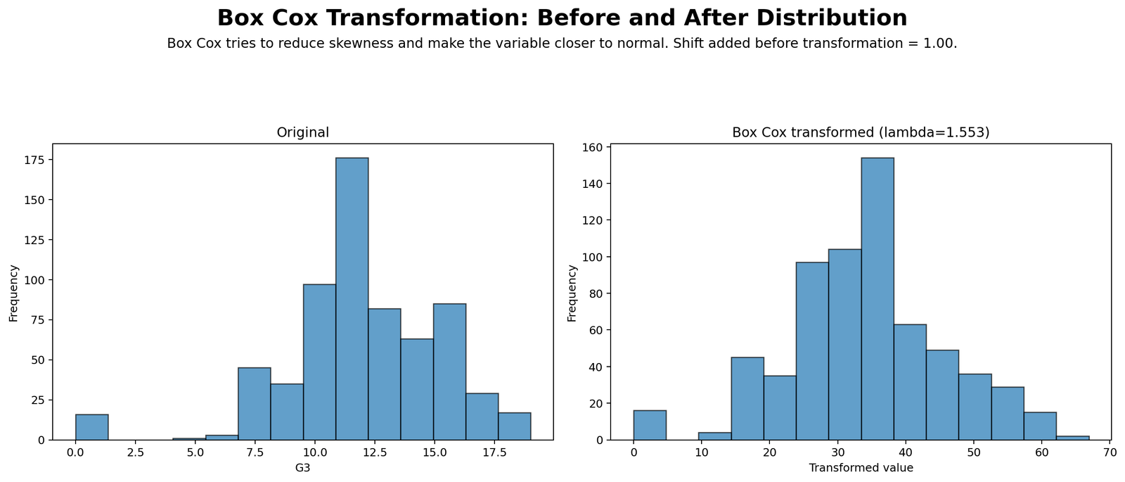
This chart compares the original G3 distribution with the transformed version. The purpose is to see whether the transformation makes the distribution more bell-shaped. In this example, the original G3 variable is bounded from 0 to 19 and has negative skewness. Because of that bounded grade scale, a Box Cox transformation does not automatically create a normal distribution.
The decision from this chart should be made with the SPSS normality output. The original G3 Shapiro-Wilk test is significant, and the transformed candidates also remain significant. Therefore, the distribution chart supports a cautious conclusion: transformation was attempted, but it should not be reported as a successful normality fix.
Python Chart 2: Before and After Q-Q Plots
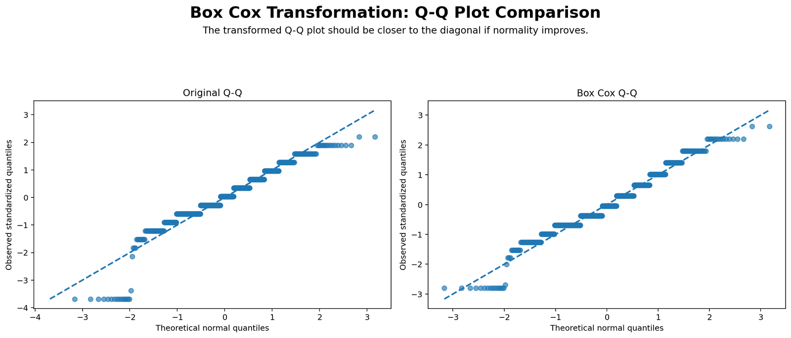
The before-after Q-Q plots show whether the transformed values align more closely with the normal reference line. A good transformation should pull points closer to the diagonal line, especially in the tails. In this example, the transformed Q-Q plot still shows substantial departures.
This agrees with the SPSS normality tests. The lambda 0 log candidate has Shapiro-Wilk W = .561, and the lambda .5 candidate has W = .791, both with p < .001. The Q-Q evidence therefore supports rejecting the idea that the tested Box Cox candidates made G3 normal. For more detail on interpreting Q-Q behavior, use Q-Q Plot Normality Check.
Python Chart 3: Lambda Log-Likelihood Curve
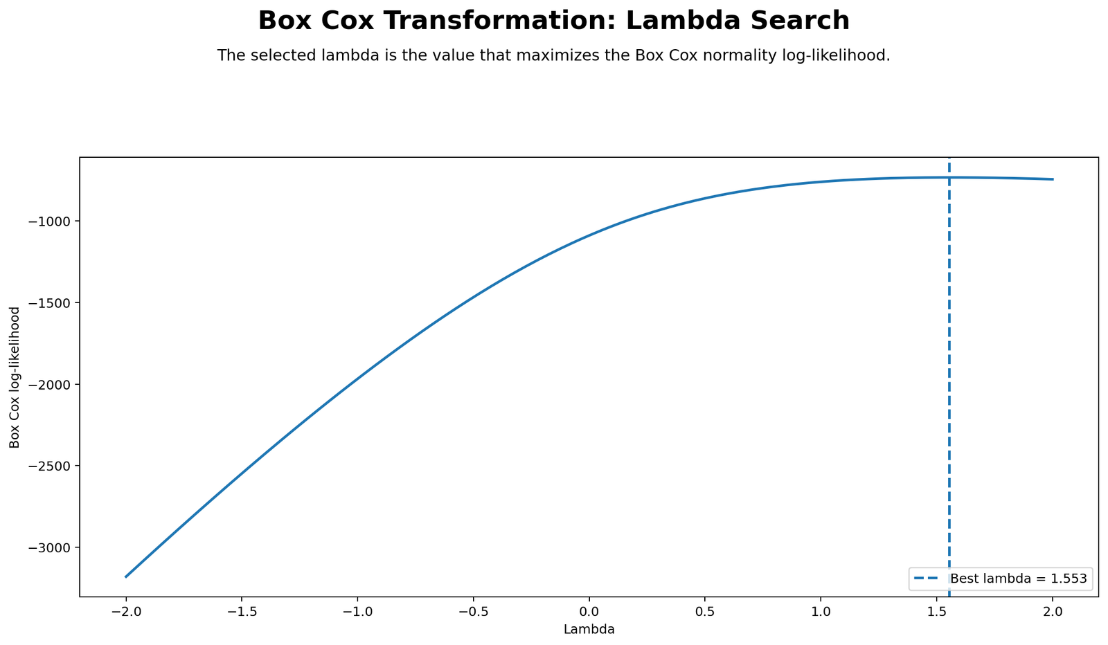
The lambda log-likelihood curve is used to identify which lambda value best fits the transformation criterion. A higher point on the curve indicates a better lambda according to the Box Cox likelihood approach. This chart is important because it shows that lambda should be estimated or evaluated, not guessed.
However, the best lambda from a likelihood curve should still be checked with normality plots and shape statistics. For G3, the SPSS candidate output shows that common candidates such as log and lambda .5 do not solve normality. The curve helps select a transformation, but the final decision depends on whether the transformation actually improves the analysis.
Python Chart 4: Skewness Before and After
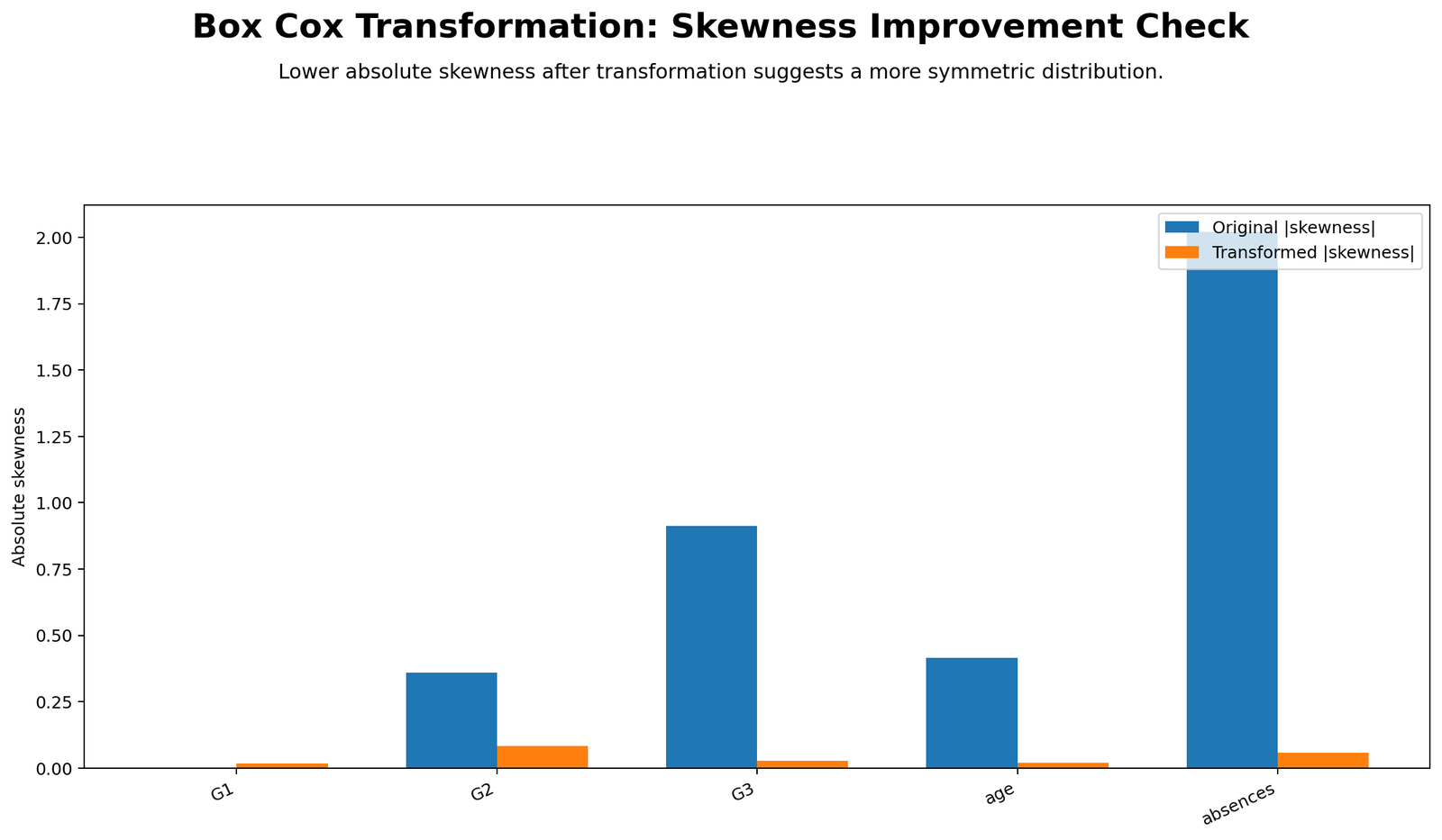
This chart is one of the clearest summaries. Original G3 has skewness = -0.913. The log candidate has skewness = -4.264, and the lambda .5 candidate has skewness = -2.369. Because the transformed candidates are more negatively skewed, the transformation does not improve the distribution shape for this variable.
The decision is straightforward: if skewness becomes worse after transformation, do not describe the transformation as successful. Instead, report that the transformation was explored and that the original scale may be preferable for interpretation, or use a method robust to non-normality.
Python Chart 5: Transformed Scores by Group

This chart shows transformed score differences by group. SPSS reports that the female group has a log candidate mean of 2.534161 and lambda .5 mean of 5.210206. The male group has a log candidate mean of 2.445754 and lambda .5 mean of 4.948868. This shows that the female group remains higher on the transformed scale.
However, transformed group means can be harder to explain than original grade means. If the transformation does not improve assumptions, reporting transformed means may reduce interpretability without improving statistical validity. Use Effect Size and Confidence Interval for clearer group reporting.
Python Chart 6: Original vs Transformed Scale
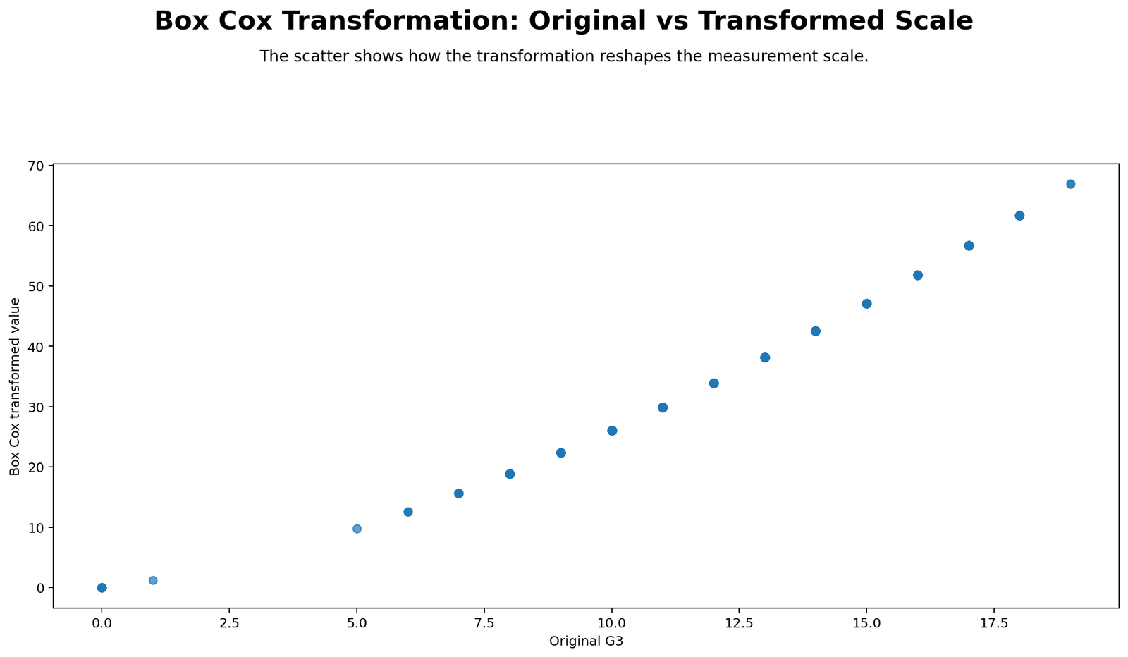
This chart explains how Box Cox changes the measurement scale. Transformation changes the spacing between values. Low, middle, and high original grades are not always separated in the same way after transformation. This is why transformed results need careful interpretation.
For G3, the transformation changes the scale but does not solve normality. Therefore, the transformed scale should not be used just because it looks mathematically advanced. The original scale is often more interpretable for grades, especially when transformation does not improve the diagnostic evidence.
R Chart-by-Chart Validation
The R charts validate the Box Cox Transformation workflow using a separate software environment. They confirm the same interpretation: transformation was evaluated, but the transformed G3 candidates should not be treated as a successful normality solution.
R Chart 1: Before and After Distribution
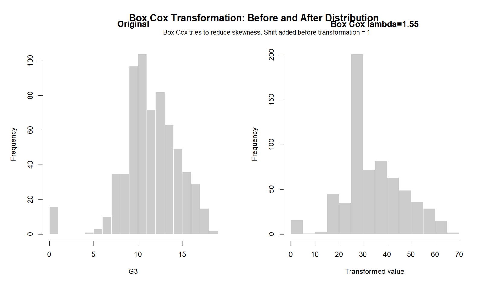
The R before-after distribution chart validates the Python distribution comparison. It confirms that changing the scale does not automatically create a normal distribution for bounded grade data.
R Chart 2: Before and After Q-Q Plots
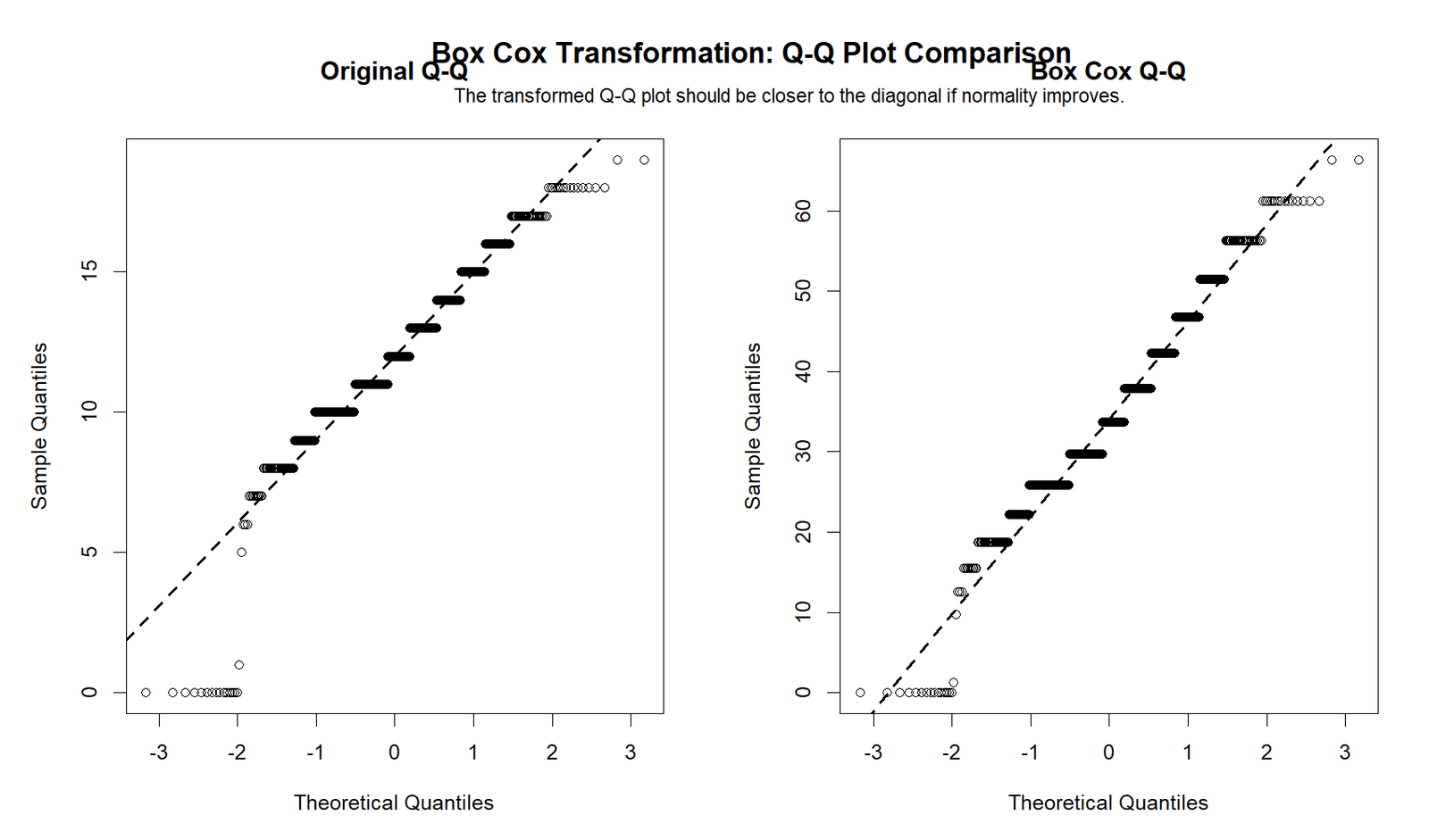
The R Q-Q plot comparison confirms that the transformed values still do not align perfectly with normal expectations. This supports the SPSS conclusion that normality remains rejected after transformation.
R Chart 3: Lambda Log-Likelihood Curve
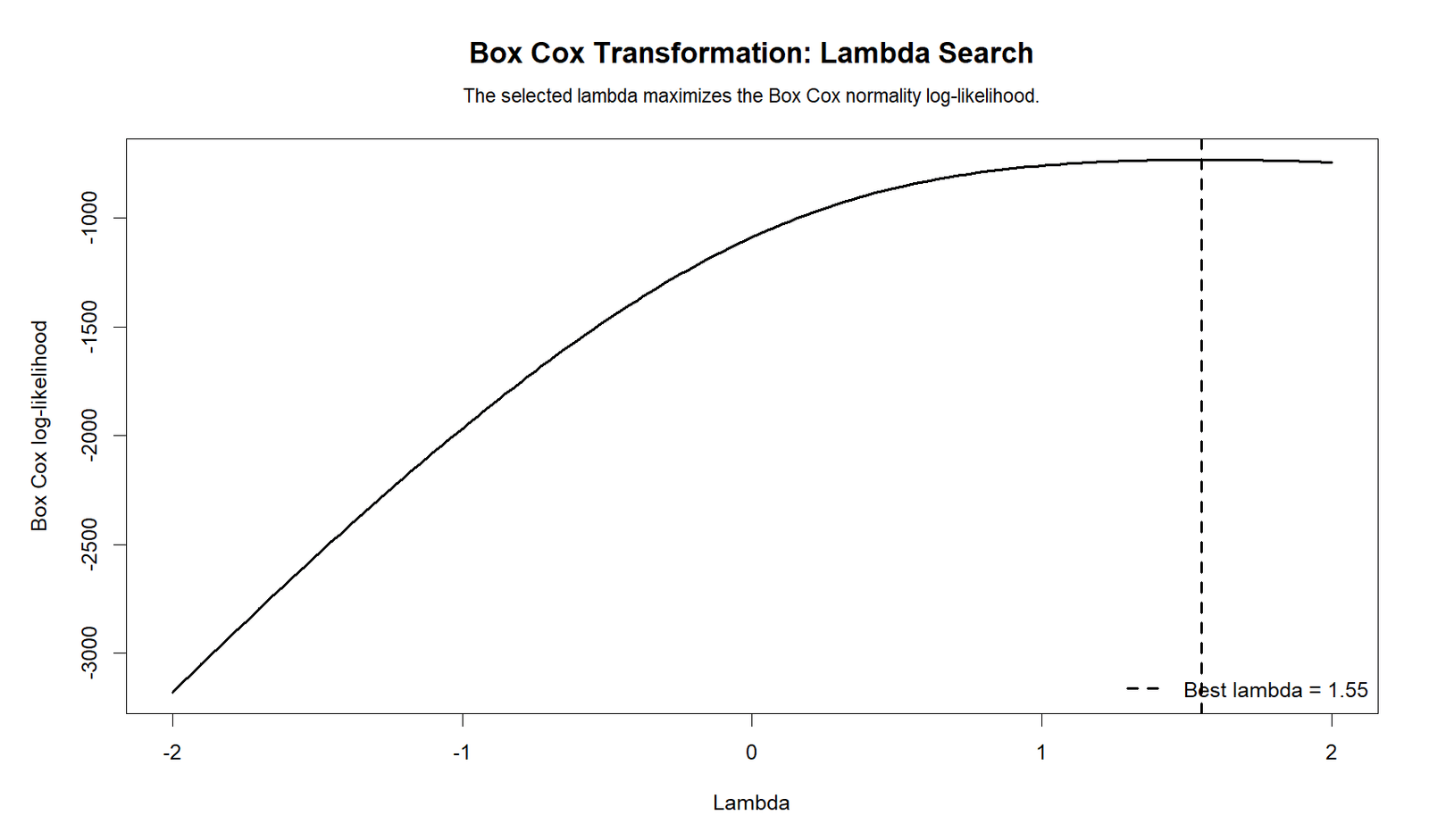
The R lambda curve validates the lambda-selection step. It reinforces the idea that Box Cox should be guided by evidence rather than arbitrary transformation choice.
R Chart 4: Skewness Before and After
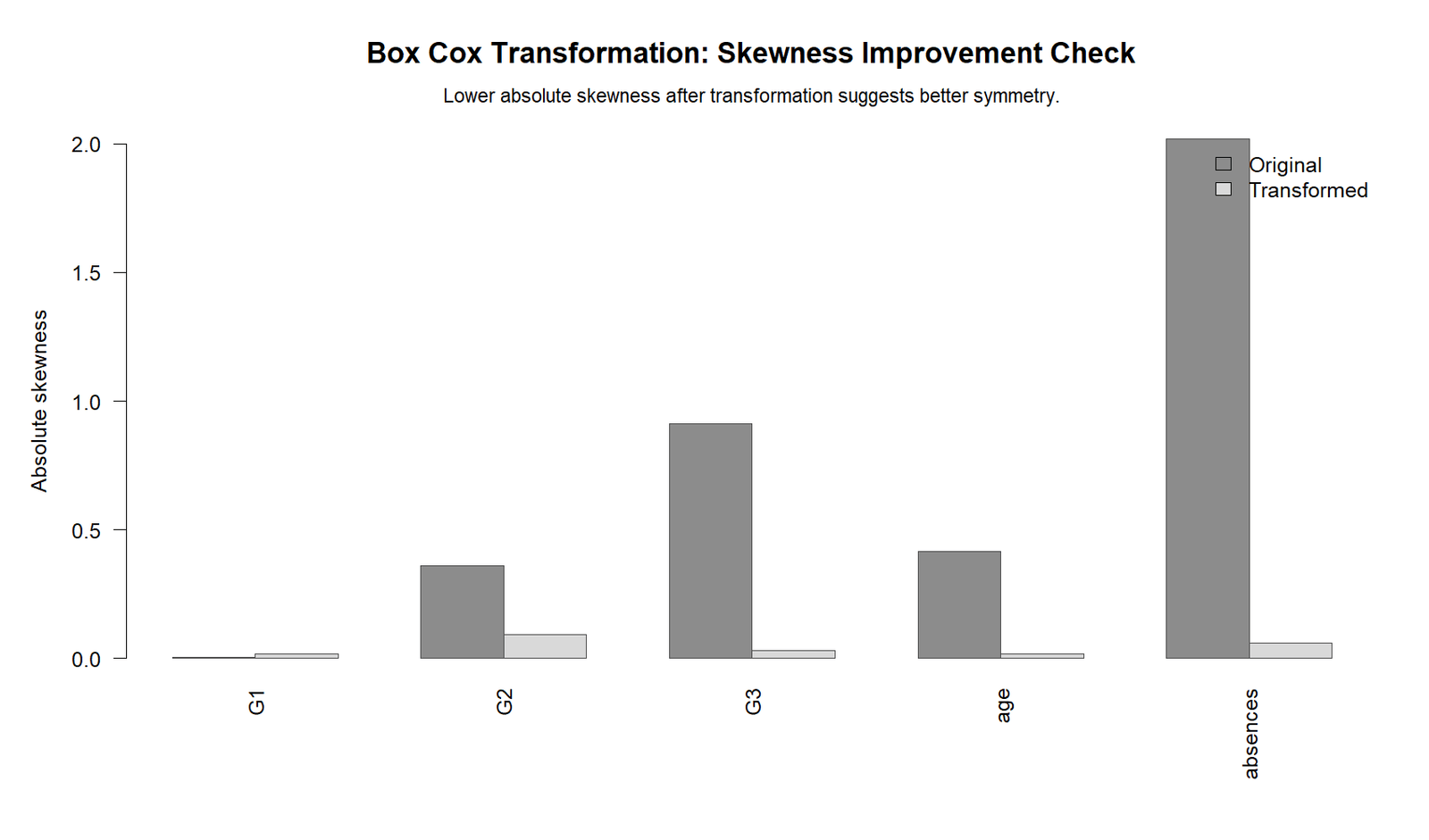
The R skewness chart validates the Python and SPSS interpretation. For G3, the transformed candidates increase negative skewness rather than reducing it. This is strong evidence against describing the transformation as successful.
R Chart 5: Original vs Transformed Scale
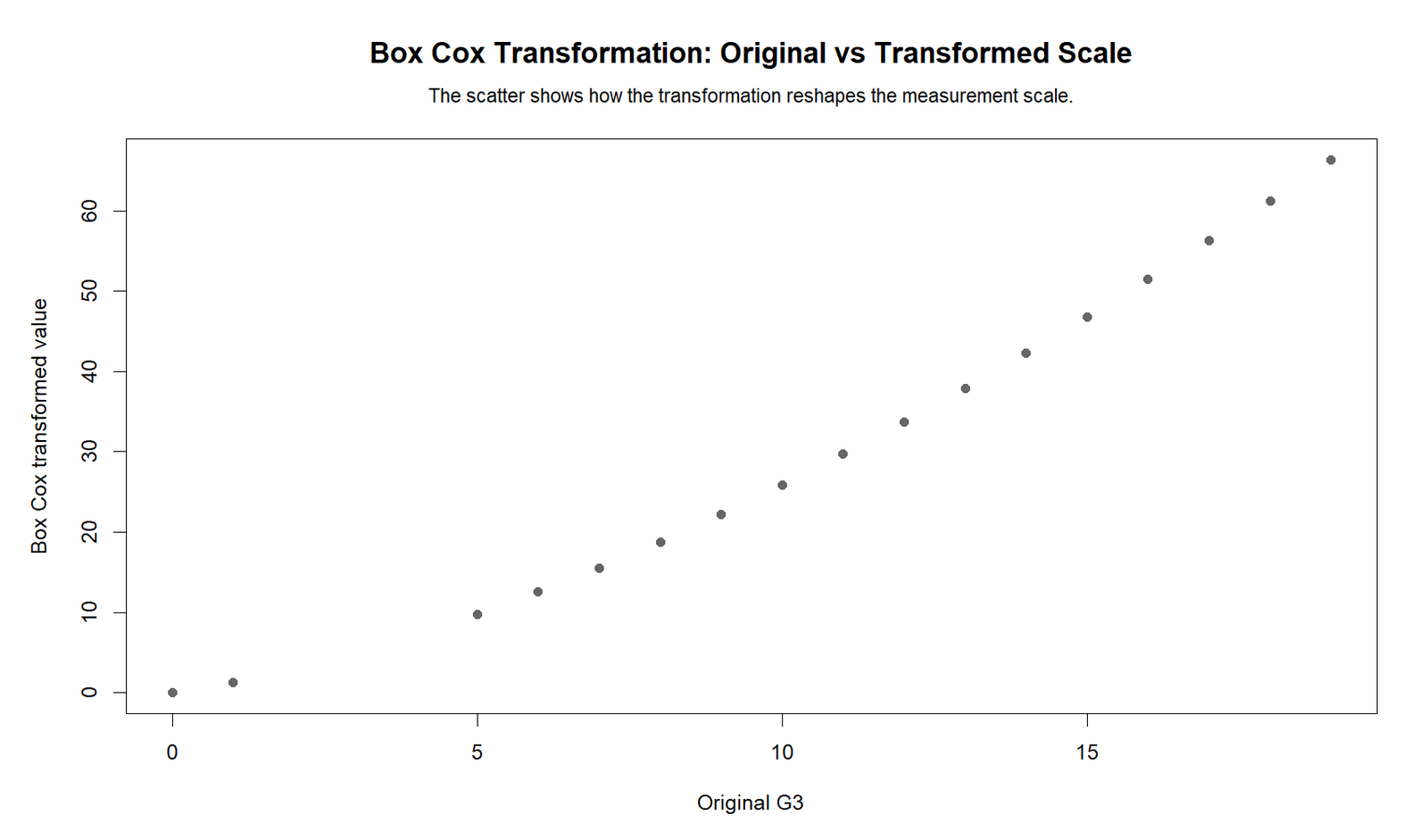
The R original-versus-transformed scale chart confirms how Box Cox changes the interpretation of values. A transformed grade score is no longer in grade points, so the result becomes less directly understandable to readers.
R Chart 6: Transformed Scores by Group

The R group chart validates the group pattern shown in Python and SPSS. Female students remain higher than male students on the transformed scale. However, because the transformation does not improve normality for G3, the original scale may still be more useful for plain-language reporting.
SPSS, R, Python and Excel Workflows for Box Cox Transformation
Box Cox Transformation can be performed in Python and R directly. SPSS can create Box Cox candidate variables manually using compute formulas. Excel can also calculate candidate transformations manually, although it does not provide a built-in lambda log-likelihood optimizer.
SPSS Workflow
| Step | SPSS Action | Purpose |
|---|---|---|
| Inspect original variable | Analyze > Descriptive Statistics > Explore | Check G3 distribution, skewness, kurtosis and normality. |
| Shift variable | COMPUTE G3_shifted = G3 + 1 | Make all values positive for Box Cox. |
| Create lambda candidates | COMPUTE transformed variables | Evaluate log, square-root and other power candidates. |
| Compare shape | Descriptives and Explore | Compare skewness, kurtosis and normality tests. |
| Report decision | APA/reporting section | Explain whether transformation improved normality. |
R Workflow
| Step | R Action | Purpose |
|---|---|---|
| Read data | read.csv() | Load the dataset. |
| Shift if needed | x_shifted <- x - min(x) + 1 | Make values strictly positive. |
| Estimate lambda | MASS::boxcox() | Find a candidate lambda from the likelihood curve. |
| Apply transformation | Box Cox formula | Create transformed variable. |
| Check normality | shapiro.test(), Q-Q plot, histogram | Evaluate whether transformation helped. |
Python Workflow
| Step | Python Action | Purpose |
|---|---|---|
| Read data | pandas.read_csv() | Load the dataset. |
| Shift if needed | x_shifted = x - x.min() + 1 | Make values positive. |
| Estimate lambda | scipy.stats.boxcox() | Apply Box Cox and estimate lambda. |
| Create charts | matplotlib | Generate before-after distributions and Q-Q plots. |
| Check normality | scipy.stats.shapiro() | Compare original and transformed normality. |
Excel Workflow
| Excel Task | Formula | Purpose |
|---|---|---|
| Shift variable | =A2-MIN($A$2:$A$650)+1 | Make values positive. |
| Log candidate | =LN(B2) | Apply lambda 0 candidate. |
| Lambda .5 candidate | =(B2^0.5-1)/0.5 | Apply square-root-style Box Cox candidate. |
| Lambda 1 candidate | =(B2^1-1)/1 | Returns original scale after shift adjustment. |
| Skewness | =SKEW(range) | Compare shape before and after. |
| Kurtosis | =KURT(range) | Compare tail behavior before and after. |
After transformation, do not rely on one statistic only. Check Descriptive Statistics, Histogram Interpretation, Q-Q Plot Normality Check, P-P Plot Normality Check, and Effect Size if the transformation will be used in a reported model.
Code Blocks for Box Cox Transformation
SPSS Syntax for Box Cox Transformation
* Box Cox Transformation candidate workflow in SPSS.
* Main variable: G3 final grade.

SET PRINTBACK=OFF MPRINT=OFF.

TITLE "Box Cox Transformation".

* Original normality.
EXAMINE VARIABLES=G3
  /PLOT BOXPLOT HISTOGRAM NPPLOT
  /COMPARE GROUPS
  /STATISTICS DESCRIPTIVES
  /CINTERVAL 95
  /MISSING LISTWISE
  /NOTOTAL.

* Shift G3 because Box Cox requires positive values.
COMPUTE G3_shifted = G3 + 1.
EXECUTE.

* Box Cox candidate transformations.
COMPUTE G3_boxcox_lam_m1 = (G3_shifted ** -1 - 1) / -1.
COMPUTE G3_boxcox_lam_m05 = (G3_shifted ** -0.5 - 1) / -0.5.
COMPUTE G3_boxcox_lam_0 = LN(G3_shifted).
COMPUTE G3_boxcox_lam_05 = (G3_shifted ** 0.5 - 1) / 0.5.
COMPUTE G3_boxcox_lam_1 = (G3_shifted ** 1 - 1) / 1.
EXECUTE.

DESCRIPTIVES VARIABLES=G3 G3_shifted G3_boxcox_lam_m1 G3_boxcox_lam_m05
  G3_boxcox_lam_0 G3_boxcox_lam_05 G3_boxcox_lam_1
  /STATISTICS=MEAN STDDEV MIN MAX SKEWNESS KURTOSIS.

* Explore main candidates.
EXAMINE VARIABLES=G3_boxcox_lam_0 G3_boxcox_lam_05
  /PLOT BOXPLOT HISTOGRAM NPPLOT
  /COMPARE GROUPS
  /STATISTICS DESCRIPTIVES
  /CINTERVAL 95
  /MISSING LISTWISE
  /NOTOTAL.

* Group comparison of transformed scores.
MEANS TABLES=G3_boxcox_lam_0 G3_boxcox_lam_05 BY sex
  /CELLS=COUNT MEAN STDDEV.

OUTPUT EXPORT
  /CONTENTS EXPORT=VISIBLE
  /PDF DOCUMENTFILE="Box-Cox-Transformation-SPSS-Output.pdf".
Python Code for Box Cox Transformation
import pandas as pd
import numpy as np
from scipy import stats

df = pd.read_csv("dataset.csv")

x = pd.to_numeric(df["G3"], errors="coerce").dropna()

# Shift to positive values because Box Cox requires x > 0
x_shifted = x - x.min() + 1

# Estimate Box Cox transformation and lambda
x_boxcox, lambda_hat = stats.boxcox(x_shifted)

print("Estimated lambda:", lambda_hat)

# Compare normality and shape
original_shapiro = stats.shapiro(x)
transformed_shapiro = stats.shapiro(x_boxcox)

print("Original Shapiro-Wilk:", original_shapiro)
print("Transformed Shapiro-Wilk:", transformed_shapiro)

summary = pd.DataFrame({
    "variable": ["original_G3", "shifted_G3", "boxcox_G3"],
    "n": [len(x), len(x_shifted), len(x_boxcox)],
    "mean": [x.mean(), x_shifted.mean(), np.mean(x_boxcox)],
    "std": [x.std(ddof=1), x_shifted.std(ddof=1), np.std(x_boxcox, ddof=1)],
    "min": [x.min(), x_shifted.min(), np.min(x_boxcox)],
    "max": [x.max(), x_shifted.max(), np.max(x_boxcox)],
    "skewness": [stats.skew(x, bias=False), stats.skew(x_shifted, bias=False), stats.skew(x_boxcox, bias=False)],
    "kurtosis": [stats.kurtosis(x, fisher=True, bias=False), stats.kurtosis(x_shifted, fisher=True, bias=False), stats.kurtosis(x_boxcox, fisher=True, bias=False)]
})

print(summary)

# Candidate transformations matching SPSS-style lambdas
candidate_lambdas = [-1, -0.5, 0, 0.5, 1]
rows = []

for lam in candidate_lambdas:
    if lam == 0:
        y = np.log(x_shifted)
    else:
        y = (np.power(x_shifted, lam) - 1) / lam

    rows.append({
        "lambda": lam,
        "mean": np.mean(y),
        "std": np.std(y, ddof=1),
        "min": np.min(y),
        "max": np.max(y),
        "skewness": stats.skew(y, bias=False),
        "kurtosis": stats.kurtosis(y, fisher=True, bias=False),
        "shapiro_w": stats.shapiro(y).statistic,
        "shapiro_p": stats.shapiro(y).pvalue
    })

candidate_table = pd.DataFrame(rows)
print(candidate_table)
R Code for Box Cox Transformation
# Box Cox Transformation in R

df <- read.csv("dataset.csv")

x <- as.numeric(df$G3)
x <- x[!is.na(x)]

# Shift to positive values
x_shifted <- x - min(x) + 1

# Candidate Box Cox function
boxcox_transform <- function(x, lambda){
  if(lambda == 0){
    return(log(x))
  } else {
    return((x^lambda - 1) / lambda)
  }
}

candidate_lambdas <- c(-1, -0.5, 0, 0.5, 1)
rows <- list()

for(lam in candidate_lambdas){
  y <- boxcox_transform(x_shifted, lam)

  rows[[as.character(lam)]] <- data.frame(
    lambda = lam,
    n = length(y),
    mean = mean(y),
    sd = sd(y),
    min = min(y),
    max = max(y),
    skewness = if(requireNamespace("e1071", quietly = TRUE)) e1071::skewness(y, type = 2) else NA,
    kurtosis = if(requireNamespace("e1071", quietly = TRUE)) e1071::kurtosis(y, type = 2) else NA,
    shapiro_w = shapiro.test(y)$statistic,
    shapiro_p = shapiro.test(y)$p.value
  )
}

candidate_table <- do.call(rbind, rows)
print(candidate_table)

# Optional lambda likelihood using MASS
# install.packages("MASS")
# library(MASS)
# model <- lm(x_shifted ~ 1)
# bc <- boxcox(model, lambda = seq(-2, 2, by = 0.1))
# best_lambda <- bc$x[which.max(bc$y)]
# print(best_lambda)
Excel Formulas for Box Cox Transformation
Assume original G3 values are in A2:A650.

Shift variable to positive values:
=B2 formula if using A values:
=A2-MIN($A$2:$A$650)+1

Lambda 0 log candidate:
=LN(B2)

Lambda 0.5 candidate:
=(B2^0.5-1)/0.5

Lambda -0.5 candidate:
=(B2^-0.5-1)/-0.5

Lambda -1 candidate:
=(B2^-1-1)/-1

Lambda 1 candidate:
=(B2^1-1)/1

Mean:
=AVERAGE(range)

Standard deviation:
=STDEV.S(range)

Skewness:
=SKEW(range)

Kurtosis:
=KURT(range)

Interpretation:
Compare original and transformed skewness, kurtosis, histogram and Q-Q plot.
Do not assume the transformed version is better unless the diagnostics improve.
APA Reporting Wording for Box Cox Transformation
When reporting Box Cox Transformation, clearly state why the transformation was attempted, how the positive-data requirement was handled, which candidates were evaluated, and whether the transformation improved normality. If it did not improve normality, say that directly.
APA-Style Transformation Attempt Report
Because G3 included zero values, the variable was shifted by adding 1 before evaluating Box Cox candidate transformations. The original G3 variable showed non-normality, Shapiro-Wilk W = .926, p < .001, with skewness = -0.913 and kurtosis = 2.712.
APA-Style Candidate Comparison Report
Box Cox candidate transformations did not improve the normality of G3. The log candidate remained non-normal, Shapiro-Wilk W = .561, p < .001, with skewness = -4.264 and kurtosis = 21.649. The lambda .5 candidate also remained non-normal, Shapiro-Wilk W = .791, p < .001, with skewness = -2.369 and kurtosis = 9.475. Therefore, the transformation was not retained as an improvement over the original scale.
Student-Friendly Report Example
A Box Cox Transformation was tested to see whether it could improve the normality of G3 final grades. Because G3 included zero values, the scores were shifted before transformation. The transformed versions remained non-normal and became more negatively skewed than the original variable. Therefore, Box Cox Transformation was not useful for improving G3 normality in this dataset.
For complete reporting, combine this transformation result with Q-Q Plot Normality Check, P-P Plot Normality Check, Effect Size, Confidence Interval, and Central Limit Theorem where relevant.
Common Mistakes in Box Cox Transformation
| Mistake | Why It Is a Problem | Correct Practice |
|---|---|---|
| Using Box Cox on zero or negative values | The formula requires strictly positive data. | Shift the variable first or choose another method. |
| Assuming transformation always improves normality | Some variables become worse after transformation. | Compare before-after diagnostics. |
| Reporting transformed results without explanation | Readers may not understand the transformed scale. | Explain lambda, shift, and interpretation. |
| Ignoring Q-Q plots | Normality tests alone do not show where departures occur. | Use Q-Q plots and histograms. |
| Forcing Box Cox on bounded grade data | Bounded discrete scales may not transform well. | Use practical judgment and robust methods when needed. |
| Confusing transformation with a hypothesis test | Box Cox itself does not produce a reject/fail decision. | Use normality tests after transformation. |
Key reminder: Box Cox Transformation is a tool, not a guarantee. It should be judged with before-after distributions, Q-Q Plot Normality Check, P-P Plot Normality Check, Kolmogorov-Smirnov Test, skewness, kurtosis, and practical interpretability.
When to Use Box Cox Transformation
Use Box Cox Transformation when the variable is strictly positive, continuous, and meaningfully skewed, especially when you need to improve model assumptions. It is commonly used before regression, ANOVA, repeated-measures modeling, or other methods where normality or variance stability matters.
| Use Box Cox When | Why It Helps | Example Decision |
|---|---|---|
| Data are strictly positive | Box Cox requires positive x values. | G3 had to be shifted because it included zero. |
| Distribution is skewed | A power transformation may reduce skewness. | Useful mainly when transformation improves skewness. |
| Residuals are non-normal | Transformation may improve model diagnostics. | Check residuals with Q-Q plots and tests. |
| Variance changes with level | Transformation may stabilize variance. | Compare with variance and heteroskedasticity diagnostics. |
| Interpretability remains acceptable | Transformed units can be harder to explain. | Do not transform if it worsens clarity and assumptions. |
Use Box Cox together with diagnostics such as Descriptive Statistics, Histogram Interpretation, Box Plot Interpretation, Q-Q Plot Normality Check, P-P Plot Normality Check, Reciprocal Transformation, Goldfeld-Quandt Test, and Ramsey RESET Test when the analysis involves regression assumptions.
Downloads and Resources for Box Cox Transformation
The resources below include the SPSS output PDF, Python charts, and R validation charts used in this guide.
Download SPSS Output PDF
Verified SPSS output for original normality, Box Cox candidates, transformed normality and group summaries.
Copy Box Cox Code
Use the SPSS, Python, R and Excel code blocks to reproduce the Box Cox Transformation workflow.
Python Chart 3: Lambda Curve
Lambda log-likelihood curve for transformation selection.
Python Chart 4: Skewness Before After
Skewness comparison showing whether transformation improved shape.
FAQs About Box Cox Transformation
What is Box Cox Transformation?
Box Cox Transformation is a power transformation used to make positive data closer to normal, reduce skewness, or improve model assumptions.
What is the Box Cox formula?
When λ is not zero, the formula is (x^λ − 1) / λ. When λ equals zero, the formula becomes ln(x).
Why did G3 need to be shifted before Box Cox Transformation?
G3 included a minimum value of 0. Box Cox requires strictly positive values, so G3 was shifted upward by adding 1.
Did Box Cox Transformation improve G3 normality in this example?
No. The tested Box Cox candidates remained non-normal and had stronger negative skewness than the original G3 scale.
What was original G3 skewness?
Original G3 skewness was -0.913.
What was the log candidate skewness?
The log-style lambda 0 candidate had skewness of -4.264, which was worse than the original scale.
What was the lambda .5 candidate skewness?
The lambda .5 candidate had skewness of -2.369, which was still more negatively skewed than original G3.
Can Box Cox Transformation be used with zero values?
Not directly. The variable must be shifted so that all values are positive before applying Box Cox.
Is Box Cox Transformation a normality test?
No. It is a transformation method. Normality must be checked after transformation using plots and tests such as Shapiro-Wilk or Kolmogorov-Smirnov.
Which plots should be checked after Box Cox Transformation?
Check before-after histograms, Q-Q plots, P-P plots, skewness, kurtosis, and normality test results.
How do I run Box Cox Transformation in Python?
Use scipy.stats.boxcox() on a strictly positive numeric vector. Shift the variable first if it contains zero or negative values.
How do I run Box Cox Transformation in R?
Use MASS::boxcox() for lambda selection and apply the Box Cox formula to a positive variable.
Can Excel calculate Box Cox candidates?
Yes. Excel can calculate candidate transformations using formulas such as =LN(x) or =(x^0.5-1)/0.5, but it does not provide a simple built-in Box Cox lambda optimizer.
Which related guides help with Box Cox Transformation?
Useful related guides include Q-Q Plot Normality Check, P-P Plot Normality Check, Kolmogorov-Smirnov Test, Reciprocal Transformation, Descriptive Statistics, and Histogram Interpretation.

